| Issue |
A&A
Volume 535, November 2011
|
|
|---|---|---|
| Article Number | A111 | |
| Number of page(s) | 9 | |
| Section | The Sun | |
| DOI | https://doi.org/10.1051/0004-6361/201116792 | |
| Published online | 21 November 2011 | |
3D MHD simulations of electric current development in a rotating sunspot: active region NOAA 8210
1
Max-Planck-Institut für Sonnensystemforschung (MPS), Katlenburg-Lindau, Germany
e-mail: This email address is being protected from spambots. You need JavaScript enabled to view it.
2 Laboratório Associado de Plasma, Instituto Nacional de Pesquisas Espaciais (INPE), São José dos Campos – SP, Brazil
e-mail: This email address is being protected from spambots. You need JavaScript enabled to view it.
3 Geophysical Institute, University of Alaska Fairbanks (UAF), Fairbanks, USA
e-mail: This email address is being protected from spambots. You need JavaScript enabled to view it.
Received: 27 February 2011
Accepted: 30 July 2011
Abstract
Context. Active region (AR) 8210 was the host of many flares and coronal mass ejections (CMEs). Studies of its temporal evolution indicated that the clockwise rotation of a negative magnetic polarity, together with the motion of a positive polarity located close to it are a major source of magnetic energy to the corona above.
Aims. Search for the mechanisms of energy storage and release above AR8210. For this sake we locate the current system generated by the photospheric plasma motion suggested as source of coronal energy supply above AR8210 and compare it with the location of identified flaring regions.
Methods. We simulated the reaction of the corona using a three-dimensional (3D) MagnetoHydroDynamic (MHD) model. The initial coronal magnetic field is extrapolated out of the observed line-of-sight (LOS) component of the photospheric magnetic field. The corresponding photospheric plasma motion is imposed close to the bottom boundary of the simulation box. Current dependent resistivity and compressibility of the plasma are considered in the model.
Results. The horizontal plasma motion causes a current system that spatially coincides with the flaring region associated to AR8210. Particularly, the rotation of the plasma over the main negative polarity gives rise to strong currents localized over the main negative polarity, i.e. close to the position of a flare site. Above this region a strong magnetic field divergence is indicated by large differential flux tube volumes. Intense currents also form along the eastern border of a positive polarity region, over a polarity inversion line (PIL), in a site where a flare appears later. The southward motion of a positive flux concentration generates a current system extending mainly along the eastern border of it, over a polarity inversion line. Magnetic energy is deposited mainly over the main negative polarity, where the major flare activity is observed at later times.
Conclusions. The two patterns of photospheric plasma motion suggested as being responsible for the flaring activity of AR8210 generate current systems spatially coincident with the flaring area associated to this active region. These currents generate magnetic fields that contribute to the increase in magnetic energy inside the simulation volume. The transport of magnetic flux by the photospheric plasma motion also contributes to the redistribution of magnetic energy. The increase in magnetic energy occurs mainly over the main negative polarity and close to where a strong current system is formed. We conclude that in the case of AR8210 the rotation of the negative polarity region is the main contributor to its flare activity. The southward motion of a positive magnetic flux concentration plays an important role in the formation of current systems at its eastern border.
Key words: Sun: corona / Sun: flares / magnetohydrodynamics (MHD) / magnetic reconnection / methods: numerical
© ESO, 2011
1. Introduction
Active region NOAA 8210 was visible on the solar disk from April 25 to May 7, 1998. During its passage over the solar disk it released many flares and CMEs as described by Warmuth et al. (2000); Thompson et al. (2000); Sterling & Moore (2001); Sterling et al. (2001); Pohjolainen et al. (2001). In the period from May 1 to 2 this active region was associated with two M-Class flares and one X-Class flare. It also created a halo CME that caused an intense magnetic storm at Earth on May 2, 1998.
Régnier & Canfield (2006) describe the evolution of magnetic fields and energetics of flares observed on May 1, 1998 in AR8210. They classify the LOS component of the photospheric magnetic field associated to AR8210 as a complex magnetic field distribution characterized by the presence of a main negative polarity region (N1) surrounded by positive polarities (P1–4). This complex magnetic field also includes a parasitic polarity (N2) that is emerging between P3 and P4. The photospheric magnetic field distribution associated to AR8210 gives rise to different connectivity domains between the main negative polarity and the positive polarities around it. The connectivity domains are divided by separatrices or quasi-separatrix layers (QSLs). Figure 2 from Régnier & Canfield (2006) shows the position of a separatrix deduced directly from EUV and soft X-ray measurements. This figure also shows the location of flares (sites A and B) and the flaring region (region F) as obtained from H-α measurements.
The photospheric plasma motion responsible for the evolution of the coronal magnetic field above NOAA AR8210 between 17:13 UT and 21:29 UT on May 1 was determined in Welsch et al. (2004), Longcope (2004), and Georgoulis & LaBonte (2006). Using the ILCT method, Welsch et al. (2004) were able to recover a clockwise rotation of the main negative polarity N1 and a southward motion of the positive polarity P1. This motion produced a shear flow around the polarity inversion line, which was suggested as being responsible for the energy injection to the corona above the active region. The amplitude of the flow velocity was around or below 1 km s-1.
Régnier & Canfield (2006) discussed a flare scenario for AR8210. In their scenario the flares are related to the rotation of the sunspot N1 and southward motion of the opposite polarity P1. The slow sunspot rotation was suggested to cause a flare by reconnection close to the separatrix.
Régnier & Priest (2007) derive the distribution of free magnetic energy and helicity for a nonlinear force-free (nlff) extrapolation of the coronal magnetic field above AR8210. They showed that the free magnetic energy stored above AR8210 corresponds to only 2.5% of the total magnetic field energy. The free energy is stored mainly in the lower corona, close to the photospheric boundary. The authors argue that, although this energy is only a small fraction of the total magnetic field energy, it is enough to trigger small C-class flares. They also calculate the photospheric vertical current density from the transverse component of the photospheric magnetic field obtained by the Mees Solar Observatory/Imaging Vector Magnetogram (MSO/IVM) on May 1, 1998 at 19:40 UT. Figure 2b from Régnier & Priest (2007) shows that the vertical component of the photospheric current exceeds 10 mA m-2. There are two regions of very localized and strong upward currents, one located over the positive polarity P1 and the other over the negative polarity N1. In between N1 and P1, there is a strong downward current.
We have tested the hypothesis of Régnier & Canfield (2006) by performing 3D MHD simulations. We investigated the consequences of plasma rotation of the main negative polarity region N1 and the southward motion of the positive polarity P1 for the development of electric currents over AR8210. We focus mainly on the spatial distribution of the global electric current system and compare its location with the location of the flaring regions in AR8210. In Sect. 2 we describe the model setup. In Sect. 3 we discuss the results obtained and, finally, in Sect. 4 we present our conclusions and summarize our main findings.
2. Model setup
The model solves the following set of resistive MHD equations (in normalized units)  \arraycolsep1.75pttogether with Ohm’s law, Ampère’s law and we take into account the ideal gas equation for a fully ionized plasma
  \arraycolsep1.75ptHere ρ is the plasma mass density, u the plasma velocity, B the magnetic field, p the thermal pressure, T the plasma temperature, and β0 the normalization value used for the plasma beta (β0 = 0.1). The polytropic index is
  . The quantity u0 denotes the velocity of a neutral gas, to which the plasma is coupled. To decrease the numerical errors we evaluate the electric current density as j = ∇ × B1, where B1 = B − BP. The field BP is the initial potential field, which is current free (∇ × BP = 0). Hence, ∇ × B1 = ∇ × B. This assumption is valid at any instant of time. The normalization of the macroscopic variables is given by B0 = 100 G, L0 = 107 m, T0 = 106 K,
  ,
,  ,
,  , and
, and  .
.
The system of equations is solved on an equidistant Cartesian grid (131 × 131 × 131 grid points) that covers a 3D volume of 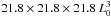 . The simulation volume presents six boundaries: four lateral, top and bottom boundaries. The lateral boundaries use line-symmetric boundary conditions (Otto et al. 2007), while the top and bottom boundaries are open. By open boundaries we mean that at the physical boundary the gradients of all quantities in the direction normal to the boundary are equal to the gradients calculated for the first layer inside the simulation box. This provides a smooth transition of the forces through the physical boundary. It is also required that ∇·B = 0 for the magnetic field.
The initial magnetic field is obtained by performing a potential extrapolation of the observed LOS component of the photospheric magnetic field. Before the extrapolation is performed, a preprocessing of the MDI/SoHO magnetogram is executed. This preprocessing includes a smoothing, a multiplication by a hanning window to remove the magnetic flux close to the boundaries, flux balance, and finally, a Fourier filtering to select only the first eight modes present in the Fourier decomposition of the MDI/SoHO magnetogram. The result is a smoothed magnetic field that maintains the main structures present in the original MDI/SoHO magnetogram but neglect small-scale features that, anyway, could not be resolved by the Eulerian grid scheme. Figure 1 shows a top view of the resulting vertical (Z-)component of the photospheric magnetic field at the bottom of the simulation box. It approximates the photospheric LOS component of the magnetic field. The lateral view at some magnetic field lines illustrates the initial potential field inside the simulation box. The positive polarities are shown in red (P11, P12, P3, P4), while the main negative polarity is shown in blue (N1). Here P11 and P12 form the positive polarity P1. Its small size means P2 is not captured in the simplified magnetic field configuration. In the figure, the position of the flares (sites A and B) and the flaring region (region F) are also indicated (see Régnier & Canfield 2006). The plasma is initially in hydrostatic equilibrium (p = const.) with constant temperature T = 0.1T0 and constant density ρ = 10ρ0. This simulation aims at a qualitative investigation of the current formation without going into detail on the thermodynamics of the corona and its dynamics. With this goal in mind, the solar gravity is neglected in the momentum equation, and the initial density and temperature is chosen in accordance with the values typical of the transition region between chromosphere and corona. Figure 2 shows the variation in plasma beta with height for a vertical cutting plane located at x = 10.9L0. As one can see in the figure, in the simulation the transition from β < 1 to β ≥ 1 takes place at heights on the order of 50 Mm, while for the typical magnitude of the magnetic field used in the simulation ( ≈ 100 G) it was expected closer to 100 Mm (Gary 2001). For the qualitative investigation of the current formation in the corona, this, however, is an acceptable deviation.
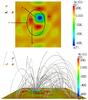 |
Fig. 1 Top panel – top view of the vertical magnetic field (color code) used to approximate the photospheric LOS component of the photospheric magnetic field of AR8210. The three positive polarities (P11–P12, P3, P4) and the main negative polarity (N1) are indicated in the figure. Also shown are the positions of the flares, sites A and B, and the flaring region, denoted by the circular F region. Bottom panel – lateral view at the vertical component of the magnetic field (color code) at the bottom of the simulation box together with selected magnetic field lines illustrating the initial potential field configuration. The lateral view is along the positive X axis. |
 |
Fig. 2 View at the simulation box in the positive X-axis direction with the coordinates given in normalized (dimensionless) units. The distribution of plasma beta is shown in a vertical cutting plane through x = 10.9L0 (1L0 = 107 m) (color coded as indicated). Above the colored region the plasma beta is larger than unity (colored in gray). Also shown is the vertical component of the magnetic field at the bottom of the simulation box and magnetic field lines colored by the corresponding value of the plasma beta. Again, gray corresponds to plasma beta over unity. |
The initial equilibrium of the system is perturbed by coupling the plasma to a background neutral gas moving in accordance with the inferred photospheric motion. The transfer of momentum between neutral gas and plasma is provided by a collision term in the momentum equation. The collision frequency between plasma and neutral gas is chosen in such a way that it is higher than the inverse of the Alfvén time for z ≤ L0, while it vanishes for z > L0. The velocity of the neutral gas is prescribed in the form of horizontal vortices for which ∇·u0 vanishes (no compression, no emerging flux).
We considered a constant background magnetic diffusivity of η ≈ 10-13 in normalized units, which correspond to η ≈ 1 m2/s in real physical units. In places where the current density is higher than 0.1j0, an anomalous resistivity is switched on, in addition to the constant background resistivity. We chose the anomalous resistivity to depend on current and its formulation is given by  (8)where η0 is the normalized value of the constant background resistivity, ηa the normalized value of the anomalous resistivity and jcrit the critical value of the current above which the anomalous resistivity is switched on. In our simulation we consider ηa = 106η0.
Our main goal is to investigate the influence of the different patterns of motion on the development of global current systems and the spatial location of these current systems compared with the spatial location of the flare activity associated with AR8210. For this sake, we performed three different numerical experiments. In the first, we imposed a velocity vortex that rotates the foot points of the field lines that are anchored in the main negative polarity region N1. The vortex rotates clockwise and has a maximum velocity of approximately 50 km s-1. In the second experiment, we imposed a velocity vortex that moves the foot points of the magnetic flux anchored in the positive polarity region P1 (P11+P12) southward. These two patterns of motion mimic the motion suggested by Régnier & Canfield (2006) as being responsible for the significant flare activity of AR8210. The last numerical experiment consisted of a combination of both patterns of motion.
3. Results
Due to the initially low values of resistivity, the plasma is almost ideally conducting. Starting from the bottom of the simulation box, magnetic flux thus moves with the plasma. This motion perturbs the magnetic field generating Alfvén waves. The Alfvénic perturbations travel along the magnetic field at the local Alfvén speed. They can be associated to electric currents according to ∇ × B. Due to the weak non ideality of the plasma, the horizontal plasma motions perpendicular to the strong vertical magnetic fields give rise to electric currents that are directed parallel to the magnetic field. However, because ∇·J = 0 has to be satisfied, the current system has to be closed by perpendicular currents. The amplitude of the currents associated to the Alfvénic perturbations depends on how abruptly the perturbations are switched on.
Regions in which the magnetic field connectivity substantially changes are important for the formation of thin current systems. Here magnetic field perturbations being generated at different regions of the solar surface can be combined to create large magnetic field gradients, hence currents (Demoulin et al. 1996; Titov et al. 2002; Büchner 2006). The width of the current sheet becomes much smaller than the characteristic length scale of the large-scale magnetic field or plasma motion applied at the photosphere (Santos et al. 2011). An appropriate measure for a changing geometry is the differential flux tube volume (Büchner 2006)  (9)To illustrate the topological structure of the field, Fig. 3 shows the differential flux tube volume calculated for the field lines starting in a plane z = L0. Regions where the differential flux tube volume present strong gradients may indicate changes in the magnetic connectivity. The flare site A and B are close to such a region of change in the connectivity of the magnetic field. It is expected that the probability of formation of strong and thin current sheets along the magnetic flux anchored on this region is higher than along magnetic flux anchored in other regions of the solar surface.
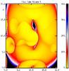 |
Fig. 3 Differential flux tube volume related to the foot points of the field lines in the plane z = L0 (1L0 = 107 m). The field of view is the same as the one showed in the top panel of Fig. 1. The values of the X-axis and Y-axis are given in normalized (dimensionless) units. |
3.1. Clockwise rotation of the main negative polarity N1
In the first numerical experiment, we imposed a velocity pattern for the neutral gas that rotates the plasma clockwise over the main negative polarity region N1. Figure 4 shows the distribution of the plasma velocity vectors at the very beginning of the simulation run. We can clearly see in the figure that the plasma is rotating clockwise over the negative polarity region.
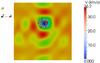 |
Fig. 4 Plasma velocity vectors for the first numerical experiment. The arrows indicate the velocity direction, and the size, and color (color bar) of the arrows indicate the velocity amplitude. Also shown is the Z component of the magnetic field at the bottom of the simulation box. |
The rotation of the plasma over the main negative polarity region generates Alfvénic perturbations that propagate along the magnetic field. The Alfvénic perturbations correspond to electric currents. The currents are mainly parallel to the magnetic field. They propagate along the field lines along with the magnetic field perturbations. Perpendicular currents close the current system. Figure 5 shows the distribution of the current density vectors at t = 618.6 s. In the figure, one can see that a current system is formed over the main negative polarity region N1. The current system extends upward and assumes the form of a fountain according to the distribution of the magnetic field lines. The strongest currents are generated in regions where the plasma is moved and at the center of the velocity vortex, close to flare site A (see Fig. 1). This is the position of major flare occurrence in AR8210. The Alfvénic perturbations of magnetic field and currents propagate along the field lines and eventually reach the flare site B (see Fig. 1), increasing the electric currents there as well.
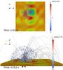 |
Fig. 5 Top (top panel) and lateral (bottom panel) views at the distribution of current density at t = 618.6 s for the first numerical experiment when plasma is rotated clockwise over the negative polarity N1. The arrows show the current density direction, the size and color of the arrows indicate the current density amplitude. Also shown are the Z component of the magnetic field at the bottom of the simulation box and the corresponding magnetic field lines. The lateral view is along the positive X axis. |
3.2. Southward motion of the positive polarity P1
In a second numerical experiment, we imposed a velocity pattern for the neutral gas that moves the plasma over the positive polarity region P11–P12 southward. Figure 6 shows the plasma velocity together with the Z component of the magnetic field at the bottom of the simulation box at the beginning of the simulation run.
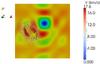 |
Fig. 6 Plasma velocity vectors for the second numerical experiment. The arrows indicate the velocity direction, and the size and color (color bar) of the arrows indicate the velocity amplitude. Also shown is the Z component of the magnetic field at the bottom of the simulation box. |
The motion of the plasma starts also to move the foot points of the magnetic flux anchored in P11 and P12. This generates a perturbation of the magnetic field that propagates along the field lines at the local Alfvén speed, which is associated to propagating electric currents. Figure 7 shows the current density vectors at t = 782.5 s in a top and a lateral view. Since the magnetic field anchored in P11 and P12 is weaker than the one anchored to N1 and the velocity amplitudes are smaller than the one used in the first numerical experiment, the currents generated in the second numerical experiment are weaker than the currents obtained in the first numerical experiment. The height of the current system is also lower because the field lines anchored in P11–P12 reach lower altitudes than the field lines anchored in N1. The figure shows that the currents develop mainly at the east border of P11–P12, over a polarity inversion line (PIL).
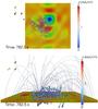 |
Fig. 7 Top (top panel) and lateral (bottom panel) views of the distribution of current density at t = 782.5 s for the second numerical experiment when plasma is moved southward over the positive polarity P11–P12. The arrows show the current direction, and the size and color of the arrows indicate the current density amplitude. Also shown are the Z component of the magnetic field at the bottom of the simulation box and corresponding magnetic field lines. The lateral view is along the positive X axis. |
3.3. Combined motion: rotation of N1 and southward motion of P1
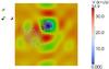 |
Fig. 8 Plasma velocity vectors for the third numerical experiment. The arrows indicate the velocity direction, and the size and color (color bar) of the arrows indicate the velocity amplitude. Also shown is the Z component of the magnetic field at the bottom of the simulation box. |
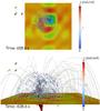 |
Fig. 9 Top (top panel) and lateral (bottom panel) views of the distribution of current density vectors obtained at t = 608.6 s for the case when plasma is rotated over the negative polarity N1 and at the same time moved southward over the positive polarity P11–P12. The arrows show the current density direction, and the size and color of the arrows indicate the current density amplitude. Also shown are the Z component of the magnetic field at the bottom of the simulation box and some of the magnetic field lines that fill the simulation box. The lateral view is along the positive X axis. |
In a third and last numerical experiment, we combined the two pattern of motion used in the first two experiments to perturb the system. Figure 8 shows the velocity vectors and the Z component of the magnetic field at the bottom of the simulation box. The amplitude of the velocity that rotates the plasma over N1 is larger than the one that moves the plasma southward over the positive polarity P11–P12. Also the magnetic field of N1 is stronger than the magnetic field of P11–P12. As a consequence one would expect that the currents resulting from the rotation of N1 will dominate the currents resulting from the southward motion of P11–P12.
Figure 9 shows the resulting distribution of the current density vectors at t = 608.6 s. Indeed, the currents generated by the rotation of the plasma over the negative polarity region dominate the currents generated by the southward motion of P11–P12. The spatial distribution of the current system is very similar to the one obtained in the first numerical experiment. Strong currents develop close to the flare sites A and B (see Fig. 1). The currents spread in the flaring region F, and owing to the configuration of the magnetic field they assume the form of a fountain.
Figure 10 shows the Z component of the magnetic field (upper panel) and electric current density (bottom panel) at the bottom boundary for t = 608.6 s. The electric current is saturated at | Jz | = 3.0 mA/m2. The resulting distribution of the vertical currents resembles very much the one obtained by Régnier & Priest (2007) using the three components of the photosperic magnetic field measured by MSO/IVM. The small differences between the results obtained from simulation and observation can be associated to our use of simplified velocity patterns and magnetic fields in the simulations, and the emergence of magnetic flux is not considered in the model.
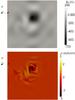 |
Fig. 10 Vertical component of the magnetic field (top panel) and vertical component of the current density (bottom panel) calculated at the bottom boundary of the simulation box, at t = 608.6 s, for the case when plasma is rotated over the negative polarity N1 and at the same time moved southward over the positive polarity P11–P12. The contour lines at the bottom panel show the position of the negative (white line) and positive (black line) polarities. |
3.3.1. Energy storage
The moving background neutral gas constantly injects energy into the system. Its coupling with the plasma via the collision term in the momentum Eq. (2) enhances the kinetic and magnetic energy of the plasma. At the beginning the plasma is at rest, and its kinetic energy is equal to zero. The initial magnetic energy inside the simulation box is the energy of a potential field (j = 0) extrapolated out of the photospheric field. However, this energy is not available to be converted into other kinds of energy because the potential field constitutes the minimum energy magnetic field configuration.
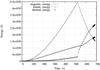 |
Fig. 11 Temporal evolution of magnetic, kinetic, and thermal energies inside a sub-volume going from z = 1.5L0 to z = 21.8L0, where (1L0 = 107 m). |
During the simulation run, the kinetic energy of the neutral gas is transferred to the plasma at the bottom part of the simulation box (0 ≤ z ≤ L0). The plasma keeps part of this energy as kinetic energy. Another part of the energy of the neutral gas is transferred to the magnetic field via Poynting flux. As a result magnetic energy accumulates in the system. The weak dissipation and compression in the plasma enhances also the thermal energy. Figure 11 shows the temporal variation of the magnetic  , thermal
  and kinetic energies
  in a sub-volume going from z = 1.5L0 to z = 21.8L0, in excess to the initial energy of the system. We did not consider the region below z = 1.5L0 in the energy analysis since we did not describe the interaction of the plasma with the neutral gas in this simulation properly. We show only the additional magnetic energy exceeding the level of the initial potential field (1.47 × 1031 J). An accurate description of the amount of free energy available would require computing the change in the potential field as well, but as a simple approximation of the change in free magnetic energy, the perturbation energy should represent a reasonable estimate. The thermal energy is also the one exceeding the level of the initial thermal energy. We consider that the energy storage period goes from t = 0 to t ≈ 522 s, even though the previous numerical experiments ran longer than this time. During this period most of the energy comes from the bottom of the simulation box (z ≤ 1.5L0), where the plasma is moved by the strong interaction with the neutral gas. Since the values of resistivity are very low, the increase in thermal energy is mainly due to compressional (adiabatic) heating.
The increase in magnetic energy inside the simulation box comes from the Poynting flux. However, magnetic energy can also be transported inside the simulation box by the plasma motion. Once the current systems are formed, the magnetic energy available to power flares and CMEs is not only the magnetic energy associated to the magnetic field generated by the currents. The magnetic field can later relax to a lower energy state for which the magnetic energy is lower than the energy of the initial potential field. This allows part of the energy of the initial potential field to be released as well. Figure 12 shows the regions of increase in magnetic energy density  inside the simulation box . We can see that magnetic energy density starts do be deposited close to the location of the flare site A. This is also the location where strong currents are formed.
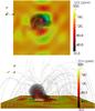 |
Fig. 12 Top (top panel) and lateral (bottom panel) views of regions of increase in magnetic energy density (Energy/Volume) inside the simulation box. Also shown is the Z component of the magnetic field at the bottom of the simulation box, together with the magnetic field lines. The lateral view is along the positive X axis. |
3.3.2. Energy release
Before t ≈ 522 s, very low values of the normalized background (η0) and anomalous (ηa) magnetic diffusivities were considered. To understand what happens when diffusive processes allow the fast relaxation of the stored energy, we increased the values of the normalized diffusivities by normalizing the physical values by the product of the expected characteristic length scale of the ion skin depth at the solar corona ( ≈ 10 m) and the characteristic Alfvén speed (v0 = vA = B0/ ). This brings the values of the normalized background and anomalous magnetic diffusivities to 1 × 10⁻⁷ and 1 × 10⁻¹, respectively. This yields a realistic estimate of the magnitude of the resistivity inside thin current layers, however, with the side effect that the resistivity operates over much larger spatial volumes (because of the limited spatial resolution) than in the real system. Taking the new values for the magnetic diffusivities into account, we started a new simulation run using as initial condition the output obtained from the previous run, for the third numerical experiment, at t = 522 s. After that time we also set the neutral gas velocity to zero, so that energy is no longer injected into the system by the interaction between plasma and neutral gas.
The new values for the background and anomalous magnetic diffusivities allow a more efficient dissipation of the magnetic field and, finally, efficient magnetic energy release by 3D reconnection. Magnetic field connectivity changes in order to straighten the magnetic field lines that were bent (twisted) due to the motion of the plasma. Concurrently, the Joule heating term in the energy equation (ηj2) increases the thermal pressure of the plasma at places where strong currents are located. The increase in thermal pressure in regions of low plasma density allow the temperature to reach peak values on the order of 107 K. The increase in the thermal pressure gives rise to pressure gradient forces that start to accelerate the plasma upward, along the field lines. The enhanced dissipation and associated magnetic reconnection start to drive the system in a characteristic time that is much shorter than that associated to the energy storage process.
Figure 13 shows the electric current densities (top left), temperature (top right), bulk velocity (bottom left), and density variation (bottom right) at t = 685.9 s. This time corresponds to approximately 160 s after we had started the simulations with the new enhanced diffusivity values. The figure shows that the main current system created by the rotation of the negative polarity (see Fig. 9) has dissipated away. Residual currents were present, and new current systems were created. However, these currents are much weaker and spatially less distributed than the original one. In the top right-hand panel of Fig. 13, there are three regions where the plasma is heated to temperatures on the order of 107 K: one region is close to the bottom boundary and located at the center of the vortex that rotates the plasma over the negative polarity N1. The other two are located a little higher in the solar atmosphere and over the polarity inversion line between P11–N1 and P3–N1.
All three regions coincide with the location of the flare site A. The strong pressure gradients generated by Joule heating cause upward plasma flows (see bottom left-hand panel in Fig. 13). The flows are directed mainly along the magnetic field lines and have amplitudes of hundreds of kilometers per second. Fast magnetoacoustic waves are generated by nonlinear coupling with the Alfvén wave. The pressure gradient forces, together with the j × B forces associated to the perpendicular currents at the front of the fast magnetoacoustic waves, redistribute the plasma inside the simulation box, creating regions of plasma density increase and depletion. From the distribution of density variation (bottom right-hand panel in Fig. 13), one can see that there are two regions of density increase (red isosurfaces). These regions take the form of two shells, which are separated by a region of density depletion. The outer overdense shell is created by the action of the j × B force associated to the perpendicular currents at the front of the fast magnetoacoustic waves. The fast magnetoacoustic waves propagate along the magnetic field lines, compressing the plasma in front of it and leaving a region of density depletion behind it. The inner overdense shell is created by the pressure gradient forces associated with the steep increase in pressure. The pressure gradients start to accelerate the plasma upward, removing even more plasma from an already density depleted region and creating an inner shell of overdense plasma. This inner shell of overdense plasma is moving at hundreds of kilometers per second and will probably work like a piston through the outer overdense shell.
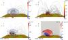 |
Fig. 13 Top left – lateral view showing the distribution of the current systems at the end of the energy release phase. The arrows show the current direction, while the size and color of the arrows show the current density amplitude. Top right – lateral view of the volume distribution of the plasma temperature at the end of the energy release phase. Bottom left – lateral view of the velocity vectors at the end of the energy release phase. The arrows show the velocity direction, while the size and the color of the arrows the velocity amplitude. Bottom right – regions of density increase (red) and depletion (blue) at the end of the energy release phase. The red (blue) isosurface shows the regions where the plasma density is four times higher (lower) than the initial one. Also shown is the Z component of the magnetic field at the bottom of the simulation box and the magnetic field lines. The view is along the positive X axis. |
The temporal variation in the magnetic, thermal, and kinetic energies during the dissipation period can be seen in Fig. 11 for t ≥ 520 s. In this phase magnetic energy is converted to thermal and kinetic energies. If we compare the length of the storage and release intervals, they are not so different in our simulations. However, we have to consider that, in order to have a much shorter run, we have used higher velocities to drive the system during the storage interval. More specifically, we used velocities that are one order of magnitude higher than those normally found on the photosphere. Consequently, we can assume that, for the characteristic velocities found on the photosphere, the storage time would be at least ten times longer than the one obtained in our simulations. This would correspond to an interval of approximately 1.4 h for the storage and 2.67 min for the release.
4. Summary and conclusions
In AR8210, the flaring region F is associated to strong photospheric magnetic fields, and for this reason it is expected that most of the flaring activity associated to AR8210 will be located there. However, inside the flaring region F there are two important flare sites, A and B, for which the question remains open why a strong flare activity happen there. Previous investigations have implied that the clockwise rotation of the negative polarity N1 and the southward motion of the positive polarity P1 could be responsible for the flares (Régnier & Canfield 2006). However, a direct association of these two motion patterns with the formation of current sheets and the storage and release of magnetic energy have never been performed.
To clarify these points and to better understand the reasons for flare eruptions in regions A and B of AR8210, we performed numerical simulations using a 3D MHD model. The initial coronal magnetic field was extrapolated out of the observed LOS component of the photospheric magnetic field. The values used for the initial plasma density, temperature, and plasma beta are close to the ones observed in the solar atmosphere. To drive the system, the corresponding photospheric plasma motion was imposed close to the bottom boundary of the simulation box. With these, we can draw the following conclusions, which shed some light on the relation between photospheric motions and the distribution of the global current systems and energetics of AR8210:
-
Both flare sites A and B are associated with large differential fluxtube volumes, indicating the influence of magnetic fieldgeometry on the occurrence of the flares.
-
The rotation of the plasma over the negative polarity N1 transports magnetic flux to the region close to the flare site A and generates a strong current channel on that region. The current channel extends along the field lines and assumes the form of a fountain following the structure of the magnetic field. Electric currents propagate mainly along the magnetic field lines, carrying Alfvénic perturbations. A strong current system starts to develop also close to the flare site B. Below the grid resolution, perhaps, intense current sheets are formed.
-
The southward motion of the positive polarity P11–P12 gives rise to a low lying current system, concentrated mainly at the east border of P11–P12, along a PIL. This current system is much weaker than the one generated by the rotation of the negative polarity N1, and does not seem to be important for the flares occurring in sites A and B.
-
The similarities between the distribution of the vertical component of the current density obtained in the simulations and the one obtained using the horizontal components of the magnetic field measured by MSO/IVM indicate that MHD simulations are, despite simplified configurations of plasma velocity and magnetic field, accurate enough to reproduce the storage and eruptive phases of flares above regions A and B.
-
During the storage period most of the energy comes from the bottom of the simulation box, where the plasma is moved by the strong interaction with the neutral gas (“chromosphere”). The switch on of higher resistivity allows enhanced energy release by 3D reconnection exactly in the place where the flare eruptions were observed. The dissipated magnetic energy is completely converted to kinetic and thermal energies, indicating no losses of energy in our simulation.
Acknowledgments
J.C.S. and A.O. thank the Max-Planck Society for funding their work by the Inter-institutional Research Initiative “Turbulent transport and ion heating, reconnection and electron acceleration in solar and fusion plasmas”, project MIF-IF-A-AERO8047. J.C.S. thanks the Conselho Nacional de Desenvolvimento Científico e Tecnológico (CNPq) for funding his work under the projects 201318/2008-3 and 481368/2010-8.
References
- Büchner, J. 2006, Space Sci. Rev., 122, 149 [NASA ADS] [CrossRef] [Google Scholar]
- Demoulin, P., Henoux, J. C., Priest, E. R., & Mandrini, C. H. 1996, A&A, 308, 643 [NASA ADS] [Google Scholar]
- Gary, G. A. 2001, Sol. Phys., 203, 71 [NASA ADS] [CrossRef] [Google Scholar]
- Georgoulis, M. K., & LaBonte, B. J. 2006, ApJ, 636, 475 [NASA ADS] [CrossRef] [Google Scholar]
- Longcope, D. W. 2004, ApJ, 612, 1181 [Google Scholar]
- Otto, A., Büchner, J., & Nikutowski, B. 2007, A&A, 468, 313 [NASA ADS] [CrossRef] [EDP Sciences] [Google Scholar]
- Pohjolainen, S., Maia, D., Pick, M., et al. 2001, ApJ, 556, 421 [NASA ADS] [CrossRef] [Google Scholar]
- Régnier, S., & Canfield, R. C. 2006, A&A, 451, 319 [NASA ADS] [CrossRef] [EDP Sciences] [Google Scholar]
- Régnier, S., & Priest, E. R. 2007, A&A, 468, 701 [NASA ADS] [CrossRef] [EDP Sciences] [Google Scholar]
- Santos, J. C., Büchner, J., & Otto, A. 2011, A&A, 525, A3 [NASA ADS] [CrossRef] [EDP Sciences] [Google Scholar]
- Sterling, A. C., & Moore, R. L. 2001, J. Geophys. Res., 106, 25227 [Google Scholar]
- Sterling, A. C., Moore, R. L., Qiu, J., & Wang, H. 2001, ApJ, 561, 1116 [NASA ADS] [CrossRef] [Google Scholar]
- Thompson, B. J., Cliver, E. W., Nitta, N., Delannée, C., & Delaboudinière, J. 2000, Geophys. Res. Lett., 27, 1431 [Google Scholar]
- Titov, V. S., Hornig, G., & Démoulin, P. 2002, J. Geophys. Res. (Space Phys.), 107, 1164 [NASA ADS] [CrossRef] [Google Scholar]
- Warmuth, A., Hanslmeier, A., Messerotti, M., et al. 2000, Sol. Phys., 194, 103 [NASA ADS] [CrossRef] [Google Scholar]
- Welsch, B. T., Fisher, G. H., Abbett, W. P., & Regnier, S. 2004, ApJ, 610, 1148 [NASA ADS] [CrossRef] [Google Scholar]
All Figures
|
Fig. 1 Top panel – top view of the vertical magnetic field (color code) used to approximate the photospheric LOS component of the photospheric magnetic field of AR8210. The three positive polarities (P11–P12, P3, P4) and the main negative polarity (N1) are indicated in the figure. Also shown are the positions of the flares, sites A and B, and the flaring region, denoted by the circular F region. Bottom panel – lateral view at the vertical component of the magnetic field (color code) at the bottom of the simulation box together with selected magnetic field lines illustrating the initial potential field configuration. The lateral view is along the positive X axis. |
| In the text | |
|
Fig. 2 View at the simulation box in the positive X-axis direction with the coordinates given in normalized (dimensionless) units. The distribution of plasma beta is shown in a vertical cutting plane through x = 10.9L0 (1L0 = 107 m) (color coded as indicated). Above the colored region the plasma beta is larger than unity (colored in gray). Also shown is the vertical component of the magnetic field at the bottom of the simulation box and magnetic field lines colored by the corresponding value of the plasma beta. Again, gray corresponds to plasma beta over unity. |
| In the text | |
|
Fig. 3 Differential flux tube volume related to the foot points of the field lines in the plane z = L0 (1L0 = 107 m). The field of view is the same as the one showed in the top panel of Fig. 1. The values of the X-axis and Y-axis are given in normalized (dimensionless) units. |
| In the text | |
|
Fig. 4 Plasma velocity vectors for the first numerical experiment. The arrows indicate the velocity direction, and the size, and color (color bar) of the arrows indicate the velocity amplitude. Also shown is the Z component of the magnetic field at the bottom of the simulation box. |
| In the text | |
|
Fig. 5 Top (top panel) and lateral (bottom panel) views at the distribution of current density at t = 618.6 s for the first numerical experiment when plasma is rotated clockwise over the negative polarity N1. The arrows show the current density direction, the size and color of the arrows indicate the current density amplitude. Also shown are the Z component of the magnetic field at the bottom of the simulation box and the corresponding magnetic field lines. The lateral view is along the positive X axis. |
| In the text | |
|
Fig. 6 Plasma velocity vectors for the second numerical experiment. The arrows indicate the velocity direction, and the size and color (color bar) of the arrows indicate the velocity amplitude. Also shown is the Z component of the magnetic field at the bottom of the simulation box. |
| In the text | |
|
Fig. 7 Top (top panel) and lateral (bottom panel) views of the distribution of current density at t = 782.5 s for the second numerical experiment when plasma is moved southward over the positive polarity P11–P12. The arrows show the current direction, and the size and color of the arrows indicate the current density amplitude. Also shown are the Z component of the magnetic field at the bottom of the simulation box and corresponding magnetic field lines. The lateral view is along the positive X axis. |
| In the text | |
|
Fig. 8 Plasma velocity vectors for the third numerical experiment. The arrows indicate the velocity direction, and the size and color (color bar) of the arrows indicate the velocity amplitude. Also shown is the Z component of the magnetic field at the bottom of the simulation box. |
| In the text | |
|
Fig. 9 Top (top panel) and lateral (bottom panel) views of the distribution of current density vectors obtained at t = 608.6 s for the case when plasma is rotated over the negative polarity N1 and at the same time moved southward over the positive polarity P11–P12. The arrows show the current density direction, and the size and color of the arrows indicate the current density amplitude. Also shown are the Z component of the magnetic field at the bottom of the simulation box and some of the magnetic field lines that fill the simulation box. The lateral view is along the positive X axis. |
| In the text | |
|
Fig. 10 Vertical component of the magnetic field (top panel) and vertical component of the current density (bottom panel) calculated at the bottom boundary of the simulation box, at t = 608.6 s, for the case when plasma is rotated over the negative polarity N1 and at the same time moved southward over the positive polarity P11–P12. The contour lines at the bottom panel show the position of the negative (white line) and positive (black line) polarities. |
| In the text | |
|
Fig. 11 Temporal evolution of magnetic, kinetic, and thermal energies inside a sub-volume going from z = 1.5L0 to z = 21.8L0, where (1L0 = 107 m). |
| In the text | |
|
Fig. 12 Top (top panel) and lateral (bottom panel) views of regions of increase in magnetic energy density (Energy/Volume) inside the simulation box. Also shown is the Z component of the magnetic field at the bottom of the simulation box, together with the magnetic field lines. The lateral view is along the positive X axis. |
| In the text | |
|
Fig. 13 Top left – lateral view showing the distribution of the current systems at the end of the energy release phase. The arrows show the current direction, while the size and color of the arrows show the current density amplitude. Top right – lateral view of the volume distribution of the plasma temperature at the end of the energy release phase. Bottom left – lateral view of the velocity vectors at the end of the energy release phase. The arrows show the velocity direction, while the size and the color of the arrows the velocity amplitude. Bottom right – regions of density increase (red) and depletion (blue) at the end of the energy release phase. The red (blue) isosurface shows the regions where the plasma density is four times higher (lower) than the initial one. Also shown is the Z component of the magnetic field at the bottom of the simulation box and the magnetic field lines. The view is along the positive X axis. |
| In the text | |
Current usage metrics show cumulative count of Article Views (full-text article views including HTML views, PDF and ePub downloads, according to the available data) and Abstracts Views on Vision4Press platform.
Data correspond to usage on the plateform after 2015. The current usage metrics is available 48-96 hours after online publication and is updated daily on week days.
Initial download of the metrics may take a while.