| Issue |
A&A
Volume 534, October 2011
|
|
|---|---|---|
| Article Number | A67 | |
| Number of page(s) | 6 | |
| Section | Planets and planetary systems | |
| DOI | https://doi.org/10.1051/0004-6361/201117374 | |
| Published online | 03 October 2011 | |
CoRoT LRa02_E2_0121: Neptune-size planet candidate turns into a hierarchical triple system with a giant primary⋆
1
School of Physics and Astronomy, Raymond and Beverly Sackler Faculty of Exact Sciences, Tel Aviv University, Tel Aviv, Israel
e-mail: This email address is being protected from spambots. You need JavaScript enabled to view it.
2
Laboratoire d’Astrophysique de Marseille, Université de Provence & CNRS, 38 rue Frédéric Joliot-Curie, 13388 Marseille Cedex 13, France
3
Observatoire de Haute Provence, CNRS/OAMP, 04870 St Michel l’ Observatoire, France
4
Observatoire de l’Université de Genève, 51 chemin des Maillettes, 1290 Sauverny, Switzerland
5
Research and Scientific Support Department, ESTEC/ESA, Keplerlaan 1, 2200AG, Noordwijk, The Netherlands
6
Oxford Astrophyiscs, Denys Wilkinson Building, Keble Road, Oxford OX1 3RH, UK
7
LESIA, Observatoire de Paris, Place Jules Janssen, 92195 Meudon Cedex, France
8
Institut d’Astrophysique Spatiale, Université Paris XI, 91405 Orsay, France
9
Instituto de Astrofísica de Canarias, 38205 La Laguna, Tenerife, Spain
10 IAG, University of São Paulo, Brasil
11
University of Vienna, Institute of Astronomy, Türkenschanzstr. 17, 1180 Vienna, Austria
12
Institute of Planetary Research, German Aerospace Center, Rutherfordstrasse 2, 12489 Berlin, Germany
13
Thüringer Landessternwarte, Sternwarte 5, Tautenburg, 07778 Tautenburg, Germany
14
Université de Nice-Sophia Antipolis, CNRS UMR 6202, Observatoire de la Côte d’Azur, BP 4229, 06304 Nice Cedex 4, France
15
Space Research Institute, Austrian Academy of Science, Schmiedlstr. 6, 8042 Graz, Austria
16
Rheinisches Institut für Umweltforschung an der Universität zu Köln, Aachener Strasse 209, 50931 Köln, Germany
17
Institut d’Astrophysique de Paris, UMR7095 CNRS, Université Pierre & Marie Curie, 98bis Bd Arago, 75014 Paris, France
18
Universidad de La Laguna, Dept. de Astrofísica, 38200 La Laguna, Tenerife, Spain
19 University of Liège, Allée du 6 août 17, Sart Tilman, Liège 1, Belgium
20
Center for Astronomy and Astrophysics, TU Berlin, Hardenbergstr. 36, 10623 Berlin, Germany
Received: 30 May 2011
Accepted: 26 July 2011
Abstract
This paper presents the case of CoRoT LRa02_E2_0121, which was initially classified as a Neptune-size transiting-planet candidate on a relatively wide orbit of 36.3 days. Follow-up observations were performed with UVES, Sandiford, SOPHIE, and HARPS. These observations revealed a faint companion in the spectra. To find the true nature of the system we derived the radial velocities of the faint companion using TODMOR – a two-dimensional correlation technique, applied to the SOPHIE spectra. Modeling the lightcurve with EBAS we discovered a secondary eclipse with a depth of ~0.07%, indicating a diluted eclipsing binary. Combined MCMC modeling of the lightcurve and the radial velocities suggested that CoRoT LRa02_E2_0121 is a hierarchical triple system with an evolved G-type primary and an A-type:F-type grazing eclipsing binary. Such triple systems are difficult to discover.
Key words: planetary systems / binaries: eclipsing / techniques: photometric / techniques: radial velocities
Based on observations made with the 1.93-m telescope at Observatoire de Haute-Provence (CNRS), France, the 3.6-m telescope at La Silla Observatory (ESO), Chile (program 184.C-0639), the VLT at Paranal Observatory (ESO), Chile (program 083.C-0690), and the 2.1-m Otto Struve telescope at McDonald Observatory, Texas, USA.
© ESO, 2011
1. Introduction
Since its launch, the CoRoT space mission (Baglin et al. 2006; Aigrain et al. 2008; Auvergne et al. 2009) has obtained more than 105 lightcurves of stars in more than 15 different fields that are spatially projected toward the center and anticenter of the Galaxy, in search of transiting exoplanets (Deleuil et al. 2011). In order to confirm a new transiting planet, a candidate has to pass a sequence of tests (e.g., Brown 2003). The tests include careful analysis of the lightcurve (Carpano et al. 2009), photometric follow-up observations (Deeg et al. 2009), and finally spectroscopic follow-up observations (Bouchy et al. 2009).
The main source of false positive alarms in the CoRoT sample are eclipsing binary systems in various configurations (Almenara et al. 2009). One possible strong indication of the binary nature of a system is the detection of a faint component in its observed spectrum. However, sometimes the stellar secondary is too faint to be noticed at first glance, and special tools are needed to detect it. Such a tool is TODMOR (e.g., Zucker & Mazeh 1994; Zucker et al. 2003, 2004), a two-dimensional correlation algorithm that was proved several times in the past to be an efficient tool for measuring the radial velocities (=RVs) of the two components of a binary system, even with a relatively faint secondary (e.g., Mazeh et al. 1995, 1997; Torres et al. 1995).
This paper presents the case of the transiting Neptune-size candidate LRa02_E2_0121 (=C0121). By careful analysis of the CoRoT lightcurve combined with spectroscopic follow-up observations of this star, we concluded that it is a hierarchical triple system with an evolved G-type primary and a grazing eclipsing binary. The case is presented here to illustrate the long curvy road one might need to travel until the true nature of a system is revealed and to demonstrate the potential of TODMOR, which can reveal the diluted-binary nature of a system with a relatively modest investment of observational resources.
Section 2 gives some details about the star and presents the CoRoT white lightcurve. Section 3 describes the spectroscopic follow-up observations and the spectral analysis. Section 4 describes our application of TODMOR to the observed SOPHIE spectra. Section 5 presents our analysis of the CoRoT lightcurve and the combined MCMC modeling of the photometric and RV data. The astrophysics of C0121 as a hierarchical triple system with a G-type giant is detailed in Sect. 6. Section 7 presents some general conclusions derived from this specific case.
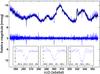 |
Fig. 1 White lightcurve of C0121. Top: the calibrated lightcurve after rebinning oversampled points back to 512 s and removing outliers. The calculated long-term trend is overplotted with a solid black line. Middle: the detrended lightcurve (for convenience the calibrated lightcurve was moved up by 10 mmag). Insets: zoom on the three individual transit-like events. |
2. The CoRoT lightcurve
The star C0121 was discovered as a transiting candidate by the alarm mode of CoRoT (Surace et al. 2008) during the LRa02 run, which lasted from Nov. 16, 2008 to Mar. 11, 2009. Its white lightcurve displayed three transit-like events of about 0.3% depth with a period of about 36.3 days, and therefore C0121 was identified as an interesting candidate of a Neptune-size planet with a relatively long period.
Figure 1 shows the calibrated and detrended white lightcurves of this candidate, with a zoom on the three transit-like events in the insets. Trends were removed with local regression that fits a second-degree polynomial to one-day-long data with weighted linear least squares. Table 1 lists some basic information on C0121.
Coordinates and magnitudes of C0121.
3. Spectroscopic follow-up observations
3.1. Radial velocity measurements
The first five RV measurements of C0121 were obtained with the SOPHIE spectrograph (Bouchy & The Sophie Team 2006; Perruchot et al. 2008), mounted at the 1.93 m telescope at the Observatoire de Haute Provence, France, between Feb. 26 and Apr. 04, 2009. Following the discovery of the transits in the alarm mode, the observations began before the end of the LRa02 run and spanned 37 days to cover a full orbital period of the transiting object. The observation timings were chosen to be close to the quadrature times of the transiting object to maximize the chance that small RV variability will be detected. These five observations gave us the first signs of the complexity of the system. Instead of the expected 36.3-day periodicity, we detected a long-term drift, with an amplitude of about 0.5 km s-1.
Six more observations of C0121 were obtained when the field was observable again, between Nov. 05 and Dec. 04, 2009. Three were acquired with SOPHIE and three other ones with the HARPS spectrograph (Pepe et al. 2000; Mayor et al. 2003), mounted at the ESO 3.6 m telescope in La Silla Observatory, Chile. All spectra had a typical signal-to-noise ratio (S/N) of 30–50 per pixel at 550 nm. In the additional six spectra we found the same long-term drift, which at that time had an observed amplitude of about 7 km s-1. The long-term variation indicated that C0121 is a member of a binary system with a long period, but did not rule out the existence of a planet in the system. There could still be a planet orbiting one of the members of the wide binary, as in the cases of 16 Cyg B (Cochran et al. 1997), γ Cephei A (Hatzes et al. 2003), or 30 Ari B (Guenther et al. 2009). Obviously, one needs more observations to understand such a complex system. Figure 2 shows the RVs of the primary, indicating that the orbital period is too long for us to derive an orbit, so we fit the measured RVs with a second-degree polynomial.
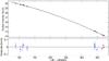 |
Fig. 2 RVs of the primary in C0121 as measured by the SOPHIE (black circles) and HARPS (red boxes) spectrographs using CCF. The solid black line is a second-degree polynomial fit. The residuals are plotted at the bottom. |
The plot started to thicken when we noticed that the three spectra taken with HARPS revealed a faint secondary. Following this, we re-analyzed the eight spectra already obtained with SOPHIE, fitting a sum of two Gaussians to the cross correlation function (=CCF, Baranne et al. 1996) derived with a G2 mask (Pepe et al. 2002). Due to the low S/N of the secondary feature in the CCF, we succeeded in measuring its RV in only 9 out of the 11 measured spectra – three from HARPS and six from SOPHIE spectra. All measured RVs are listed in Table 2.
The nine measured velocities of the faint secondary were consistent with the 36.3-day period found by CoRoT, but with a large RV semiamplitude of ~62 km s-1. This finding ruled out completely the existence of a transiting planet in C0121, and indicated that the extremely shallow transit-like signal is coming from its faint companion, which is by itself a diluted eclipsing binary.
Along the way we found one more surprise: the measured RVs of the faint companion of C0121 were in anti-phase with the CoRoT lightcurve; i.e., the detected eclipses occurred on the rising part of the RV curve. This means that the eclipses detected in the CoRoT lightcurve are caused by the star whose spectrum is detected in the composite spectra of the system, passing in front of its companion. The spectrum of the eclipsed star is not seen in the observed spectra. This is a very unusual case, because in most eclipsing binaries the primary eclipse occurs when the primary star, whose spectrum dominates the spectra, is eclipsed.
It was clear then that C0121 includes at least three stars. To facilitate the discussion we denoted the primary star in the spectra by C0121-A, the secondary star in the spectra, whose RV was observed to vary with a large amplitude by C0121-Bb, and the eclipsed star during the primary eclipses detected so far by C0121-Ba.
The measured RVs of C0121 (km s-1).
3.2. High-resolution spectroscopic observations
A reconnaissance high-resolution (R ≈ 47 000) spectrum of C0121 was acquired on February 13, 2009, using the Sandiford Cassegrain echelle spectrograph (McCarthy et al. 1993) mounted at the 2.1 m Otto Struve Telescope at McDonald Observatory. The analysis of the spectrum revealed a G-type giant star with Teff = 5500 ± 250 K, log g = 3.0 ± 0.2, and vsini = 12 ± 1 km s-1.
Furthermore, high-resolution, high-S/N spectroscopy of C0121 was performed with the UVES spectrograph (Dekker & D’Odorico 1992) mounted at the ESO 8.2 m Very Large Telescope (=VLT) in Paranal Observatory, Chile. Two consecutive exposures of 3000 s each were acquired on April 8, 2009, under the ESO program 083.C-0690. The adopted set-up yielded a resolving power of R ≈ 67 000 in the spectral range of 3280 − 6820 Å, with a final S/N of about 320 per pixel at 5500 Å. Following the procedure already adopted in some CoRoT discovery papers (e.g., Deleuil et al. 2008; Gandolfi et al. 2010), the UVES spectrum was used to derive the fundamental photospheric parameters of C0121. Ignoring the additional light from C0121-Ba and C0121-Bb, we found Teff = 5640 ± 100 K, log g = 2.9 ± 0.1, [M/H] = −1.0 ± 0.2, and vsini = 11.5 ± 1.0 km s-1, corresponding to a G0 III star. Allowing a dilution factor and fitting only the Mg I, Fe I/II and Ca I lines we found Teff = 4980 ± 100 K, log g = 2.6 ± 0.1, [M/H] = −0.5 ± 0.2, and vsini = 11.0 ± 1.0 km s-1, corresponding to a G8 III star.
The two observations indicate that C0121-A is probably a G-type giant star.
4. TODMOR analysis of the SOPHIE spectra
To better understand the unusual C0121 system, we analyzed all eight SOPHIE spectra with our two-dimensional correlation algorithm TODMOR, and derived the RVs of C0121-Bb from all eight spectra. Our best model included as the primary template the observed spectrum of HD 32923, a G4V star (White et al. 2007), rotationally broadened by 9 km s-1, and as the secondary template the observed spectrum of HD 185395 (θ Cyg), an F4V star (Kupka et al. 2004). The secondary/primary flux ratio was ~ 0.07.
Despite our efforts, we did not detect any spectral signature of C0121-Ba, even when analyzing the data with TRIMOR (Mazeh et al. 2009), an algorithm to analyze multi-order spectra of triple systems. This might indicate that Ba is a substantially hotter star, with spectral type A or even earlier. Such stars have only few broad spectral lines in the optical band, and therefore it is hard to measure their RVs, especially when their light is blended with the light of other stars.
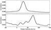 |
Fig. 3 TODMOR plot for the first exposure of C0121. The upper and lower panels show the primary and secondary cuts through the two-dimensional correlation function. |
Figure 3 shows the TODMOR results for the first SOPHIE exposure of C0121. The upper and lower panels of the figure show primary and secondary cuts through the two-dimensional correlation function that run through the correlation peak. The primary cut (upper panel) is parallel to the primary RV axis, freezing the secondary velocity at its derived velocity. The secondary cut (lower panel) runs parallel to the secondary RV axis, freezing the primary velocity at its derived velocity.
We note that in the upper panel the correlation drops by ~0.6 when moving away from the peak, because we change the velocity of the primary template in the model. On the other hand, the correlation in the lower panel drops only by ~0.002, because we change the velocity of the secondary template, which contributes only ~7% of the light, and the primary velocity is kept at its best value. Nevertheless, the peak at the lower panel is prominent, indicating the high significance of the detection of the secondary velocity.
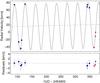 |
Fig. 4 RVs of C0121-Bb as measured by the SOPHIE (black circles) and HARPS (red boxes) spectrographs. SOPHIE RVs were derived with TODMOR, while HARPS RVs were derived by fitting a sum of two Gaussians to the CCF. The solid line is the Keplerian model produced from the orbital parameters in Table 3 and the dashed line is the center-of-mass velocity. The residuals are plotted at the bottom. |
The TODMOR RVs of C0121-A and C0121-Bb are listed in Table 2. Figure 4 presents the RVs of C0121-Bb with our best orbital solution, which is described in the next section.
We also estimated the effective temperatures of C0121-A and C0121-Bb from the SOPHIE spectra by trying a range of high-resolution PHOENIX synthetic models (Hauschildt & Baron 1999) with different Teff values as templates. TODMOR found Teff,A = 5650 ± 200 K and Teff,Bb = 6500 ± 500 K, in agreement with the analysis of the UVES and Sandiford observations.
5. Modeling the eclipsing binary C0121-B
To estimate the photometric parameters of C0121-B we re-analyzed the CoRoT white lightcurve with EBAS (Tamuz et al. 2006; Mazeh et al. 2006), an algorithm for analyzing eclipsing-binary lightcurve based on the EBOP subroutines (Popper & Etzel 1981). Our EBAS analysis discovered a faint secondary eclipse with a depth of (0.07 ± 0.01)% at the orbital phase ~0.52, showing again that C0121-B is actually an eclipsing binary (see Fig. 5). The CoRoT lightcurve covered three primary and four secondary eclipses.
The parameters of C0121-B from the combined lightcurve and RV modeling.
Final parameters were derived with MCMC analysis (e.g., Tegmark et al. 2004; Ford 2005) of the white lightcurve, together with the RV data. The input data were the detrended white lightcurve from CoRoT, which included 19 348 points and the 11 measured RVs of C0121-Bb. From the RVs listed in Table 2 we used the 8 TODMOR-derived SOPHIE RVs and the 3 CCF-derived HARPS RVs. Errors for the photometric data were derived from the local scatter of the detrended lightcurve (see Fig. 1).
The sizes of the MCMC Gaussian perturbations were set by the error estimations of EBAS and by a relatively short MCMC run (of ~105 accepted steps). Following the Metropolis-Hastings algorithm, trial points with lower χ2 were accepted, whereas trial points with higher χ2 were accepted only with probability of exp( − Δχ2/2), assuming the observational errors to be Gaussian (Ford 2005). The χ2 for each trial point was the sum of the lightcurve χ2 and the χ2 of the RV data. We used flat prior distributions for all free parameters of the model, all detailed in Table 3. The absolute values of ecosω, esinω, Js, rt, k, x and L3 were constrained to be between 0 and 1.
The fractional sum of radii (rt) and the impact parameter (x) can be expressed by the more conventional parameters as  (1)and
  (2)where Rp and Rs are the primary and secondary radii, a is the orbital semimajor axis, i the inclination, e the eccentricity, and ω the longitude of periastron (Tamuz et al. 2006). Using this convention, x = 1 when the components are grazing but not yet eclipsing. We used linear limb darkening law, with coefficients, up and us, fixed according to Sing (2010), assuming an A5 and F5 dwarfs for the primary and secondary stars in the eclipsing binary.
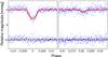 |
Fig. 5 Zoom on the primary and secondary eclipses in the phase-folded lightcurve of C0121 with our best model overplotted with a solid red line. The residuals were moved down by 10 mmag for convenience. |
The MCMC run consisted of 2 × 10⁶ accepted steps. The derived value of each parameter was its MCMC median, and its confidence limits were estimated as the range of MCMC values that cover the central 68.3% of the chain.
Table 3 gives the full list of the estimated parameters of C0121-B from the MCMC analysis. Most of the model parameters showed normal posterior probability distribution. For the ones with skewed distribution, Table 3 gives uneven confidence limits. Figure 5 presents the folded lightcurve and our best model, zoomed on the primary and secondary eclipses.
We note that the high x value we found indicates that the C0121-B eclipsing binary is grazing. In addition, the significantly non-zero center-of-mass acceleration value we found indicates that the C0121-B binary is itself a member of a hierarchical triple system.
The time of periastron passage (T), as well as some other parameters of C0121-B, which are listed at the bottom of Table 3, were analytically calculated for each point in the MCMC chain. Their values and errors were estimated the same way as for the free parameters of the model. Only for the Bb:Ba flux ratio did we take the most probable value of Js k2 as our estimation, where Js is the Bb:Ba surface-brightness ratio and k their ratio of radii (see Table 3), and not the median one, because we found its probability distribution to be extremely skewed.
C0121 was bright enough for CoRoT to observe it with its three different bands (e.g., Aigrain et al. 2008; Bordé et al. 2010). The reduction of the colored lightcurves, which was done after the completion of the LRa02 run, revealed different depths of the primary eclipse – (0.42 ± 0.02)% in blue, (0.35 ± 0.02)% in green, and (0.18 ± 0.02)% in red, indicating again that C0121-Ba is probably hotter than the other two stars in the system.
6. The C0121 system
The light of C0121 is coming from (at least) three stellar sources: a G-type star (C0121-A) on a wide orbit with an unknown period and an eclipsing binary (C0121-B) that includes an F-type star (C0121-Bb) orbiting a hotter and more massive star (C0121-Ba) on a nearly circular orbit of ~ 36.3 days. In addition, the center of mass of the C0121-B system is itself on a wide orbit with unknown period. We explore now the assumption that the three observed stars, A, Ba, and Bb, consist of a single hierarchical triple system. To do that, we use the following previously-estimated quantities and relations, derived from the white lightcurve and spectra of C0121:
-
the effective temperature of C0121-Bb is 6500 ± 500;
-
the effective temperature of C0121-A is 5650 ± 200;
-
the Bb:Ba surface-brightness ratio is 0.61 ± 0.23;
-
the Bb:Ba flux ratio is
 ;
; -
C0121-A contributes 86 ± 4% of the total light of the system;
-
the Ba:Bb mass ratio q depends on MBb through (MBbf-1sin3i) q3 − q2 − 2q − 1 = 0, where the mass function f is 0.903 ± 0.022 M⊙ and the inclination i is 87.4 ± 0.4°;
-
the center-of-mass acceleration of C0121-B is 20.6 ± 2.8 m s-1 d-1;
-
the average acceleration value of C0121-A is − 25 ± 1 m s-1 d-1.
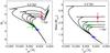
Fig. 6 Y2 stellar isochrones from Demarque et al. (2004) for solar metallicity ( [Fe/H] = 0.05, [α/Fe] = 0) and ages of 0.2,0.4,0.6,0.8, and 1 Gyr, from top-left to bottom-right. Left: MV(Teff) isochrones. Right: M(Teff) isochrones. Our estimations for C0121-A, C0121-Ba, and C0121-Bb are marked by a red diamond, a green square, and a blue circle, respectively. The absolute magnitude and mass of C0121-Bb were taken as the average value of the isochrones for a 6500 K star, assuming no error.
-
the MV brightness of Bb is 3.7;
the mass of Bb is 1.3 M⊙.
 K. From the assumed MV value of Bb, and using the derived brightness ratios, we got for C0121-Ba and C0121-A an MV values of
  and
and  , respectively. From the assumed mass of Bb and the derived ratios, including the acceleration ratio between A and B, we got for C0121-Ba and C0121-A masses of 2.25 ± 0.04 M⊙ and 2.8 ± 0.4 M⊙, respectively.
To see whether the three temperatures, brightnesses, and masses can be fitted on a single isochrone, we plotted the Y2 stellar isochrones for solar metallicity and ages of 0.2–1 Gyr in Fig. 6, together with our estimations for the effective temperatures, masses, and MV values of the three observed stars. It can be seen that a single isochrone of ~ 0.6 Gyr could fit all nine estimated values, supporting the hierarchical triple hypothesis.
Another way to estimate the stellar temperatures is to use the lightcurves of the different CoRoT bands. We derived the six Js, j and L3,j values, where j indicates the color, using MCMC as before, and searched for the best temperatures of the three stars, together with the best Ba:A ratio of radii, kBa:A, similar to the way we estimated Teff, Ba from the white lightcurve parameters. To do that we had to estimate the wavelength range of the blue, green, and red CoRoT bandpasses. From the observed magnitudes of C0121 in each channel, we estimated the two effective wavelengths that separate the channels in the CoRoT mask to be roughly at 5100 and 5600 Å. We got Teff, A = 5700 ± 200 K, Teff,Ba = 7200 ± 400 K, Teff, Bb = 6500 ± 300 K, and kBa:A = 0.20 ± 0.02. These values agree with the above estimated values and confirm that C0121-A is indeed a G-type giant star.
The visual and absolute magnitudes of C0121-A yield a distance of  kpc to the system, consistent with being in the Perseus arm of the Galaxy (Russeil 2003).
7. Conclusions
The available photometric and spectral information for C0121 indicates that the system is a hierarchical triple system and that the distant companion, C0121-A, is a G-type giant star. Hierarchical triple systems with the distant component in its giant phase are quite difficult to discover. Even if the close pair is an eclipsing binary, the dilution factor makes the eclipse rather shallow. In our case the (grazing) eclipse depth is only ~ 0.3%. Very recently, Derekas et al. (2011) discovered a similar case, HD 181068, for which the observed depth of the close-pair eclipse was also much less than 1%. Not surprisingly, the triple nature of HD 181068 was also discovered by a lightcurve obtained from space, this time with the Kepler mission. Ground-based observations could not have detected the eclipses of the close binary in these systems. When the close pair is not eclipsing it is almost impossible to detect the triple nature of the system if the distant companion is a giant, even if the wide orbital period is short enough to be discovered by radial-velocity observations of the giant. The discoveries of these two systems indicate that triple systems might not be rare, as already found by Mayor & Mazeh (1987), Tokovinin (2008), and Raghavan et al. (2010).
The present case demonstrates how a promising Neptune-size transiting-planet candidate turned out to be a grazing eclipsing binary in a hierarchical triple system. Indeed, hierarchical triple systems are expected to be the main source for false positive detections of Neptune-size transiting-planet candidates in the Kepler data too (Morton & Johnson 2011). The true nature of the system could have been revealed by analyzing the first few SOPHIE spectra with TODMOR, suggesting that an automated TODMOR pipeline could be useful in the long planet-hunting procedure. We hope to construct such a pipeline in the near future, so we can detect disguised hierarchical triple systems as early as possible.
Acknowledgments
We thank Gil Sokol, Gil Nachmani, and Simchon Faigler for their help with the lightcurve analysis. This research was supported by the Israel Science Foundation (grant No. 655/07). Financial support for the SOPHIE observations from the “Programme National de Planétologie” (PNP) of CNRS/INSU, France is gratefully acknowledged. We also acknowledge support from the French National Research Agency (ANR-08-JCJC-0102-01). The German CoRoT Team acknowledges the support of DLR grants 50OW204 and 50OW603. We thank the anonymous referee for fruitful comments and suggestions.
References
- Aigrain, S., Barge, P., Deleuil, M., et al. 2008, in 14th Cambridge Workshop on Cool Stars, Stellar Systems, and the Sun, ed. G. van Belle, ASP Conf. Ser., 384, 270 [Google Scholar]
- Almenara, J. M., Deeg, H. J., Aigrain, S., et al. 2009, A&A, 506, 337 [NASA ADS] [CrossRef] [EDP Sciences] [Google Scholar]
- Auvergne, M., Bodin, P., Boisnard, L., et al. 2009, A&A, 506, 411 [NASA ADS] [CrossRef] [EDP Sciences] [Google Scholar]
- Baglin, A., Auvergne, M., Boisnard, L., et al. 2006, in 36th COSPAR Scientific Assembly, 36, 3749 [Google Scholar]
- Baranne, A., Queloz, D., Mayor, M., et al. 1996, A&AS, 119, 373 [NASA ADS] [CrossRef] [EDP Sciences] [Google Scholar]
- Bordé, P., Bouchy, F., Deleuil, M., et al. 2010, A&A, 520, A66 [NASA ADS] [CrossRef] [EDP Sciences] [Google Scholar]
- Bouchy, F., & The Sophie Team 2006, in Tenth Anniversary of 51 Peg-b: Status of and prospects for hot Jupiter studies, ed. L. Arnold, F. Bouchy, & C. Moutou, 319 [Google Scholar]
- Bouchy, F., Moutou, C., Queloz, D., & the CoRoT Exoplanet Science Team 2009, in IAU Symp., 253, 129 [Google Scholar]
- Brown, T. M. 2003, ApJ, 593, L125 [NASA ADS] [CrossRef] [Google Scholar]
- Carpano, S., Cabrera, J., Alonso, R., et al. 2009, A&A, 506, 491 [NASA ADS] [CrossRef] [EDP Sciences] [Google Scholar]
- Cochran, W. D., Hatzes, A. P., Butler, R. P., & Marcy, G. W. 1997, ApJ, 483, 457 [NASA ADS] [CrossRef] [Google Scholar]
- Cutri, R. M., Skrutskie, M. F., van Dyk, S., et al. 2003, 2MASS All Sky Catalog of point sources [Google Scholar]
- Deeg, H. J., Gillon, M., Shporer, A., et al. 2009, A&A, 506, 343 [NASA ADS] [CrossRef] [EDP Sciences] [Google Scholar]
- Dekker, H., & D’Odorico, S. 1992, The Messenger, 70, 13 [NASA ADS] [Google Scholar]
- Deleuil, M., Deeg, H. J., Alonso, R., et al. 2008, A&A, 491, 889 [NASA ADS] [CrossRef] [EDP Sciences] [Google Scholar]
- Deleuil, M., Meunier, J. C., Moutou, C., et al. 2009, AJ, 138, 649 [NASA ADS] [CrossRef] [Google Scholar]
- Deleuil, M., Moutou, C., & Bordé, P. 2011, Detection and Dynamics of Transiting Exoplanets, St. Michel l’Observatoire, France, ed. F. Bouchy, R. Díaz, & C. Moutou, EPJ Web Conf., 11, 1001 [Google Scholar]
- Demarque, P., Woo, J., Kim, Y., & Yi, S. K. 2004, ApJS, 155, 667 [NASA ADS] [CrossRef] [Google Scholar]
- Derekas, A., Kiss, L. L., Borkovits, T., et al. 2011, Science, 332, 216 [NASA ADS] [CrossRef] [PubMed] [Google Scholar]
- Ford, E. B. 2005, AJ, 129, 1706 [Google Scholar]
- Gandolfi, D., Hébrard, G., Alonso, R., et al. 2010, A&A, 524, A55 [NASA ADS] [CrossRef] [EDP Sciences] [Google Scholar]
- Guenther, E. W., Hartmann, M., Esposito, M., et al. 2009, A&A, 507, 1659 [NASA ADS] [CrossRef] [EDP Sciences] [Google Scholar]
- Hatzes, A. P., Cochran, W. D., Endl, M., et al. 2003, ApJ, 599, 1383 [NASA ADS] [CrossRef] [Google Scholar]
- Hauschildt, P. H., & Baron, E. 1999, J. Comput. Appl. Math., 109, 41 [NASA ADS] [CrossRef] [Google Scholar]
- Kupka, F., Landstreet, J. D., Sigut, A., et al. 2004, in The A-Star Puzzle, ed. J. Zverko, J. Ziznovsky, S. J. Adelman, & W. W. Weiss, IAU Symp., 224, 573 [Google Scholar]
- Mayor, M., & Mazeh, T. 1987, A&A, 171, 157 [NASA ADS] [Google Scholar]
- Mayor, M., Pepe, F., Queloz, D., et al. 2003, The Messenger, 114, 20 [NASA ADS] [Google Scholar]
- Mazeh, T., Zucker, S., Goldberg, D., et al. 1995, ApJ, 449, 909 [NASA ADS] [CrossRef] [Google Scholar]
- Mazeh, T., Martin, E. L., Goldberg, D., & Smith, H. A. 1997, MNRAS, 284, 341 [NASA ADS] [CrossRef] [Google Scholar]
- Mazeh, T., Tamuz, O., & North, P. 2006, MNRAS, 367, 1531 [NASA ADS] [CrossRef] [Google Scholar]
- Mazeh, T., Tsodikovich, Y., Segal, Y., et al. 2009, MNRAS, 399, 906 [NASA ADS] [CrossRef] [Google Scholar]
- McCarthy, J. K., Sandiford, B. A., Boyd, D., & Booth, J. 1993, PASP, 105, 881 [NASA ADS] [CrossRef] [Google Scholar]
- Michel, E., Samadi, R., Baudin, F., et al. 2009, A&A, 495, 979 [NASA ADS] [CrossRef] [EDP Sciences] [Google Scholar]
- Morton, T. D., & Johnson, J. A. 2011, ApJ, 738, 170 [NASA ADS] [CrossRef] [Google Scholar]
- Pepe, F., Mayor, M., Delabre, B., et al. 2000, in SPIE Conf. Ser. 4008, ed. M. Iye, & A. F. Moorwood, 582 [Google Scholar]
- Pepe, F., Mayor, M., Galland, F., et al. 2002, A&A, 388, 632 [NASA ADS] [CrossRef] [EDP Sciences] [Google Scholar]
- Perruchot, S., Kohler, D., Bouchy, F., et al. 2008, SPIE Conf. Ser., 7014 [Google Scholar]
- Popper, D. M., & Etzel, P. B. 1981, AJ, 86, 102 [NASA ADS] [CrossRef] [Google Scholar]
- Raghavan, D., McAlister, H. A., Henry, T. J., et al. 2010, ApJS, 190, 1 [NASA ADS] [CrossRef] [EDP Sciences] [Google Scholar]
- Russeil, D. 2003, A&A, 397, 133 [NASA ADS] [CrossRef] [EDP Sciences] [Google Scholar]
- Sing, D. K. 2010, A&A, 510, A21 [Google Scholar]
- Surace, C., Alonso, R., Barge, P., et al. 2008, SPIE Conf. Ser., 7019 [Google Scholar]
- Tamuz, O., Mazeh, T., & North, P. 2006, MNRAS, 367, 1521 [NASA ADS] [CrossRef] [Google Scholar]
- Tegmark, M., Strauss, M. A., Blanton, M. R., et al. 2004, Phys. Rev. D, 69, 103501 [CrossRef] [Google Scholar]
- Tokovinin, A. 2008, MNRAS, 389, 925 [NASA ADS] [CrossRef] [Google Scholar]
- Torres, G., Stefanik, R. P., Latham, D. W., & Mazeh, T. 1995, ApJ, 452, 870 [NASA ADS] [CrossRef] [Google Scholar]
- White, R. J., Gabor, J. M., & Hillenbrand, L. A. 2007, AJ, 133, 2524 [NASA ADS] [CrossRef] [Google Scholar]
- Zucker, S., & Mazeh, T. 1994, ApJ, 420, 806 [NASA ADS] [CrossRef] [EDP Sciences] [MathSciNet] [Google Scholar]
- Zucker, S., Mazeh, T., Santos, N. C., Udry, S., & Mayor, M. 2003, A&A, 404, 775 [NASA ADS] [CrossRef] [EDP Sciences] [Google Scholar]
- Zucker, S., Mazeh, T., Santos, N. C., Udry, S., & Mayor, M. 2004, A&A, 426, 695 [NASA ADS] [CrossRef] [EDP Sciences] [MathSciNet] [Google Scholar]
All Tables
All Figures
|
Fig. 1 White lightcurve of C0121. Top: the calibrated lightcurve after rebinning oversampled points back to 512 s and removing outliers. The calculated long-term trend is overplotted with a solid black line. Middle: the detrended lightcurve (for convenience the calibrated lightcurve was moved up by 10 mmag). Insets: zoom on the three individual transit-like events. |
| In the text | |
|
Fig. 2 RVs of the primary in C0121 as measured by the SOPHIE (black circles) and HARPS (red boxes) spectrographs using CCF. The solid black line is a second-degree polynomial fit. The residuals are plotted at the bottom. |
| In the text | |
|
Fig. 3 TODMOR plot for the first exposure of C0121. The upper and lower panels show the primary and secondary cuts through the two-dimensional correlation function. |
| In the text | |
|
Fig. 4 RVs of C0121-Bb as measured by the SOPHIE (black circles) and HARPS (red boxes) spectrographs. SOPHIE RVs were derived with TODMOR, while HARPS RVs were derived by fitting a sum of two Gaussians to the CCF. The solid line is the Keplerian model produced from the orbital parameters in Table 3 and the dashed line is the center-of-mass velocity. The residuals are plotted at the bottom. |
| In the text | |
|
Fig. 5 Zoom on the primary and secondary eclipses in the phase-folded lightcurve of C0121 with our best model overplotted with a solid red line. The residuals were moved down by 10 mmag for convenience. |
| In the text | |
|
Fig. 6 Y2 stellar isochrones from Demarque et al. (2004) for solar metallicity ( [Fe/H] = 0.05, [α/Fe] = 0) and ages of 0.2,0.4,0.6,0.8, and 1 Gyr, from top-left to bottom-right. Left: MV(Teff) isochrones. Right: M(Teff) isochrones. Our estimations for C0121-A, C0121-Ba, and C0121-Bb are marked by a red diamond, a green square, and a blue circle, respectively. The absolute magnitude and mass of C0121-Bb were taken as the average value of the isochrones for a 6500 K star, assuming no error. |
| In the text | |
Current usage metrics show cumulative count of Article Views (full-text article views including HTML views, PDF and ePub downloads, according to the available data) and Abstracts Views on Vision4Press platform.
Data correspond to usage on the plateform after 2015. The current usage metrics is available 48-96 hours after online publication and is updated daily on week days.
Initial download of the metrics may take a while.