| Issue |
A&A
Volume 534, October 2011
|
|
|---|---|---|
| Article Number | A9 | |
| Number of page(s) | 15 | |
| Section | Galactic structure, stellar clusters and populations | |
| DOI | https://doi.org/10.1051/0004-6361/201116714 | |
| Published online | 21 September 2011 | |
Photometric signatures of multiple stellar populations in Galactic globular clusters⋆,⋆⋆
1
Zentrum für Astronomie der Universität Heidelberg, Landessternwarte, Königstuhl 12, 69117 Heidelberg, Germany
e-mail: This email address is being protected from spambots. You need JavaScript enabled to view it.
2
Max-Planck-Institut für Astrophysik, Karl-Schwarzschild-Str. 1, 85748 Garching, Federal Republic of Germany
3
GEPI, Observatoire de Paris, CNRS, Université Paris Diderot, Place Jules Janssen, 92190 Meudon, France
4
Astrophysics Research Institute, Liverpool John Moores University, Twelve Quays House, Egerton Wharf, Birkenhead CH41 1LD, UK
5
INAF – Osservatorio Astronomico di Collurania, via M. Maggini, 64100 Teramo, Italy
Received: 14 February 2011
Accepted: 1 April 2011
Abstract
We calculated synthetic spectra for typical chemical element mixtures (i.e., a standard α-enhanced distribution, and distributions displaying CN and ONa anticorrelations) found in the various subpopulations harboured by individual Galactic globular clusters. From the spectra we determined bolometric corrections to the standard Johnson-Cousins and Strömgren filters and finally predicted colours. These bolometric corrections and colour-transformations, coupled to our theoretical isochrones with the appropriate chemical composition, provided us with a complete and self-consistent set of theoretical predictions for the effect of abundance variations on the observed cluster colour–magnitude diagrams. CNO abundance variations affect mainly wavelengths shorter than ~400 nm owing to the rise of molecular absorption bands in cooler atmospheres. As a consequence, colour and magnitude changes are largest in the blue filters, independently of using broad or intermediate bandpasses. Colour–magnitude diagrams involving uvy and UB filters (and their various possible colour combinations) are therefore best suited to infer photometrically the presence of multiple stellar generations in individual clusters. They are particularly sensitive to variations in the N abundance, with the largest variations affecting the red giant branch (RGB) and lower main sequence (MS). BVI diagrams are expected to display multiple sequences only if the different populations are characterized by variations of the C+N+O sum and/or helium abundance that lead to changes in luminosity and effective temperature, but leave the flux distribution above 400 nm practically unaffected. A variation of just the helium abundance up to the level we investigate here exclusively affects the interior structure of stars, and is largely irrelevant for the atmospheric structure and the resulting flux distribution in the whole wavelength range spanned by our analysis.
Key words: stars: abundances / Hertzsprung-Russell and C-M diagrams / stars: evolution / globular clusters: general
Table A.1 is available in electronic form at http://www.aanda.org
The synthetic fluxes (FITS files) are only available at the CDS via anonymous ftp to cdsarc.u-strasbg.fr (130.79.128.5) or via http://cdsarc.u-strasbg.fr/viz-bin/qcat?J/A+A/534/A9
© ESO, 2011
1. Introduction
It is now widely accepted that Galactic globular clusters (GCs) host multiple stellar populations which display the effects of cluster internal chemical evolution. The majority of GCs appear to have two approximately coeval subpopulations, or rather, two generations of stars. The recognition of this fact came with the increasing observational evidence for what was called “star-to-star abundance variations” or “abundance anomalies”, which manifest themselves as variations of nitrogen, oxygen, and sodium, and in some clusters of magnesium and aluminum abundances. Lithium has been found to vary in a few cases (NGC 6752, NGC 6397, and 47 Tucanae, Pasquini et al. 2005; Bonifacio et al. 2007; Lind et al. 2009; Shen et al. 2010), anticorrelating with sodium, and hints exist that elements as heavy as sulfur might be affected (in 47 Tuc, Sbordone et al. 2009). These abundance variations are found in stars of all evolutionary stages. An extensive discussion of these anticorrelations, their interpretation as two generations of cluster stars, and the connection with structural cluster parameters can be found in Carretta et al. (2010b), who also quote a comprehensive list of original papers (see also the review by Gratton et al. 2004). It is remarkable that the investigation by Carretta et al. (2010b), which included over 1200 red giants in 19 carefully selected clusters, revealed that the “primordial” population is generally the less numerous one, comprising typically 30% of all cluster members. In contrast, 50–70% belong to the “intermediate population”, defined as showing an overabundance of [Na/Fe] of more than 4σ (σ being the typical star-to-star error in [Na/Fe]-determination for each cluster; see Carretta et al. 2009) above the mean abundance observed in field stars with the same iron content. In some clusters, e.g., M 13 and NGC 2808, the anomalies reach extreme values, in which case the remaining stars are counted as an “extreme population”, and – at least in the case of NGC 2808 (see the following discussion) – they could be representative of a third generation of stars, distinct from the primordial and the intermediate ones.
These element variations in clusters have been known for a few decades (e.g., in M 3 and M 13, Cohen 1978), mainly through spectroscopic analyses of cluster members, the number of which has steadily increased, in particular because of the availability of high-resolution multi-object spectrographs. Nevertheless, the actual fraction of cluster stars investigated is still very small. Additional evidence that GCs host multiple populations came from high-quality photometric data for thousands of cluster stars. Anderson (1998) discovered that the broad main sequence (MS) of the (untypical) cluster ω Cen may actually be composed of two separate sequences.Lee et al. (1999) identified these sub-populations in the cluster red giant branch (RGB) and pointed out analogies with NGC 2808 and M 22 CMDs, which were to be confirmed almost a decade later. Bedin et al. (2004) and follow-up work demonstrated that the two sequences have different metallicities, with the bluer one surprisingly hosting the more metal-rich population ( [Fe/H] = −1.26 as compared to − 1.57 of the bulk of the cluster population). The only explanation found so far (Norris 2004; Piotto et al. 2005) is that the bluer sequence has a higher helium mass fraction Y ≈ 0.38, compared to a normal value of 0.25. A weakly populated third main-sequence, redder than the two others, was found by Villanova et al. (2007) and was definitely confirmed on the basis of an accurate WFC3 photometry by Bellini et al. (2010). ω Cen is also known for hosting at least four subgiant (Lee et al. 2005; Sollima et al. 2005; Villanova et al. 2007; Bellini et al. 2010) and red giant branches (see Johnson et al. 2009, for a recent compilation), which differ not only in metal content, but probably also in age. While these empirical findings, the cluster mass, and the undisputable presence of a spread in iron content definitely put ω Cen in a special position among GCs, the photometric evidence for several subpopulations is clear and has led to similar investigations in other massive clusters.
As it turned out, multiple cluster sequences in the CMDs are indeed present in several other clusters. So far, they have been detected in NGC 2808 (three main-sequences; D’Antona et al. 2005; Piotto et al. 2007), NGC 1851 (double SGB and RGB Milone et al. 2008; Han et al. 2009), M 4, NGC 3201 and NGC 1261 (two red giant branch populations; Marino et al. 2008; Kravtsov et al. 2010a,b), as well as in NGC 6752 and 47 Tuc (clear spread of the MS, also RGB spread in NGC 6752; Anderson et al. 2009; Milone et al. 2010b; Kravtsov et al. 2011). In a number of cases (e.g., NGC 1261, NGC 3201, NGC 6752, see Kravtsov et al. 2010b,a, 2011), evidence exists that the two populations also have different radial distributions, with the redder RGB population being more centrally concentrated. Aside from the aforementioned NGC 1851, Piotto (2008), Marino et al. (2009) and Milone et al. (2010a) announced preliminary findings of multiple subgiant branches in seven more clusters, among them M 22, M 54, 47 Tuc, NGC 6388. These object do not display as dramatic a Fe abundance spread as the one found in ω Cen, although M 22 seems to display an abundance spread of about 0.2 dex, correlating with the abundance of s-process elements (Da Costa et al. 2009; Marino et al. 2009). The question therefore is, what could cause the photometric splitting? A second question concerns the fact that the splitting and/or broadening of main-sequences, subgiant branches, and red giant branches, is not present in all photometric colours, a circumstantial evidence that rules out the presence of a large age difference between the subpopulations as the cause for the splitting.
The internal chemical evolution of the clusters that led to the different abundances in the two stellar generations has affected only lighter elements up to Al and can be directly linked to high temperature proton-capture nucleosynthesis. In the two scenarios that potentially could explain the chemical properties, this implies an increased helium content in the material from which the second generation is formed. These currently discussed options are winds from massive stars or mass loss from intermediate mass stars during the thermally pulsing asymptotic giant branch phase (AGB – see, e.g., Renzini 2008, and references therein). The increase in helium could range between being marginal up to the postulated value for the blue MS in ω Cen and the bluest MS in NGC 2808, and could be as high as Y = 0.38 (Piotto et al. 2007). Therefore, both the spectroscopic and the photometric evidence for multiple cluster populations are intimately linked to the same mechanism.
For these reasons it is interesting to investigate the way in which the photometric properties of cluster isochrones depend on abundance variations. They can be used to separate subpopulations for further spectroscopic investigations, to verify known or suspected chemical compositions, or to assess the fraction of first and second generation stars in a cluster. They may also help in understanding the origin of multiple MS, subgiant- and red giant branches within one cluster. Salaris et al. (2006) and Pietrinferni et al. (2009) calculated stellar tracks and isochrones for chemical compositions showing the CN- and ONa-anticorrelations, as well as for enhanced helium mixtures. They demonstrated that in the Johnson-Cousins filters V and I only an extreme helium enhancement leads to a significant colour change as compared to a standard Pop. II mixture. They also predicted slight changes in the RGB bump position, and a separation of first and second generation stars along the horizontal branch. Cassisi et al. (2008) used these isochrones to explain the splitting of the subgiant branch (SGB) in NGC 1851 as a consequence of enhanced C+N+O abundances. Ventura et al. (2009) further investigated this question, constraining the total C+N+O abundance and the maximum helium content compatible with the MS width. From the observational side, while Yong et al. (2009) claim a variation in this sum by a factor of 4, Villanova et al. (2010) dispute any evidence for this. Needless to say that for the AGB-pollution scenario it is of great importance whether the sum of the CNO-elements in the second generation stars is constant or has increased due to He-burning products.
All isochrone computations mentioned so far treated the actual chemical composition consistently in the stellar interior models. In particular, appropriate Rosseland mean opacities were used. Dotter et al. (2007) investigated in detail the influence of individual element abundances. This limits a strict comparison of isochrones to the theoretical Hertzsprung-Russell-diagram (HRD). However, for the precise prediction of colours, also stellar atmospheres and spectra with consistent chemical composition are needed. This is of particular importance because there is a clear evidence for the existence of a correlation between splittings of evolutionary sequences in colour magnitude diagrams (CMDs) involving “blue” photometric bands (such as the standard U Johnson band) and abundance anticorrelations, while these photometric peculiarities disappear when using visual bands like V and I (see among others the case of M 4, Marino et al. 2008).
This work presents the first determinations of bolometric corrections and colours for widely used blue to near-infrared standard filters from synthetic spectra with chemical compositions typical of both first and second generation stars found in GCs. Although we are postponing a detailed comparison with observed clusters, our results already allow a basic comparison with observations and specific predictions. The structure of the paper is as follows: the next two sections (2 and 3) present the methodology of our analysis and a description of the theoretical model atmosphere and synthetic spectrum calculations, respectively. Application of these spectral calculations to isochrones representative of first and second generation stars follows in Sect. 4, before a summary and discussion of the results closes the paper.
Mass and number fractions (normalized to unity) for the three metal mixtures considered.
2. Methodology
We considered a reference isochrone from the BaSTI database1 (Pietrinferni et al. 2006), with the following characteristics: an age of 12 Gyr, helium mass fraction Y = 0.246 and metal mass fraction Z = 0.001, which results in an iron abundance of [Fe/H] = −1.62 for the α-enhanced metal mixture of the BaSTI models ([α/Fe] ~ 0.4). Such an isochrone is representative for the first generation population in a typical Galactic GC. A second generation of GC stars is represented by coeval (i.e. 12 Gyr old) isochrones calculated for the same [Fe/H] = −1.62, Y = 0.246, but with two different choices for a metal distribution, in which the elements C, N, O, and Na follow observed (anti-)correlations. We also included an additional case for a mixture with CNONa anticorrelations and, additionally, an increased initial He abundance of Y = 0.400 (see Fig. 1).
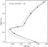 |
Fig. 1 Theoretical isochrones from the MS to the tip of the RGB for the four different chemical compositions. The solid line corresponds to both the reference first-generation population and the second-generation population with the CNONa2 metal mixture (both with Y = 0.246), because they are virtually identical. The black dots along this isochrone denote the points for which we calculated the model atmosphere and synthetic spectra. The dashed line corresponds to the second- generation population with the CNONa1 metal mixture (Y = 0.246), while the dash-dotted line is for the same population, but for an initial He mass fraction of Y = 0.40.(See the text for more details.) |
Abundances for selected elements in the four chemical mixtures used for the atmosphere computations.
The three metal mixtures (mass fraction of metals normalized to unity) are listed in Table 1. The α-enhanced mixture employed in the BaSTI database (Pietrinferni et al. 2006), which corresponds to typical first-generation subpopulations in Galactic GCs, is labelled as “reference”. The first mixture representative of second-generation stars is labelled “CNONa1”, and displays – compared to the reference α-enhanced mixture – enhancements of N and Na by 1.8 dex and 0.8 dex by mass, respectively, together with depletions of C and O by 0.6 dex and 0.8 dex, respectively. This is the same metal distribution already used in the calculations by Salaris et al. (2006) and Pietrinferni et al. (2009). An alternative composition for second-generation stars is labelled “CNONa2”; it is the same as the CNONa1 mixture but for the enhancement of N that in this case is equal to 1.44 dex by mass. The important difference between CNONa1 and CNONa2 “second-generation” mixtures is that in the first case, at fixed Fe abundance, the C+N+O mass fraction is enhanced by a factor of 2 compared to the reference composition, whereas the CNONa2 mixture has the same CNO content (in both number and mass fractions) as the reference composition, within 0.5%. This also implies (given that the C+N+O sum constitutes most of the total metal content) that for Y = 0.246 as in the reference first-generation composition, the total metal mass fraction Z of isochrones for the CNONa1 mixture has to be larger than the reference composition by a factor 1.84, to have [Fe/H] = −1.62. Both CNONa1 and CNONa2 mixtures are representative of extreme values of the CNONa anticorrelations observed in Galactic GCs (Carretta et al. 2005, 2010b). In particular, spectroscopic measurements of the C+N+O sum in individual GCs typically find values in first- and second-generation stars that are within a factor of ~2 (Carretta et al. 2005) – which is the typical error bar in these estimates.
In case of the CNONa2 mixture, the metal distribution was constructed specifically to keep the same Z as the reference composition when Y = 0.246. As for the CNONa1 metal mixture, we also considered the case of an enhanced helium mass fraction Y = 0.400.Here we also imposed the condition of having [Fe/H] = −1.62 as in the reference composition, which implies a metallicity Z larger by a factor 1.46. The final mixtures are given in Table 2.
Strictly speaking, our choice of keeping [Fe/H] = −1.62 for the CNONa1 mixture with enhanced helium does not agree with scenarios that could explain the chemical signatures of the second generation stars. In these models Fe and all other iron-peak elements are not affected, and indeed the absolute iron-abundance should be kept constant, so that an increase of Y accompanied by a decrease in hydrogen abundance would affect [Fe/H]. So far, there is only one highly significant empirical evidence that shows the existence of differences in [Fe/H] between distinct subpopulations within a GC, e.g, the case of NGC 2808 (Bragaglia et al. 2010). This has been interpreted as caused by significant changes of the initial helium abundance between the various subpopulations, as we already discussed in the introduction. It is also important to notice that almost all chemical abundance studies so far were based on scaled solar composition model atmospheres, at most including α-enhancement. If a population displays a large enough departure from the scaled solar composition, a failure to account for the true chemical pattern in the model atmosphere could potentially skew the derived [Fe/H], possibly masking differences in [Fe/H] among populations.
At any rate, even for our choice of an extreme He enhancement, by varying Y and keeping Z fixed one would obtain a variation of [Fe/H] of about 0.1 dex. We verified from the α-enhanced Castelli & Kurucz (2004) models that such a small variation of [Fe/H] affects the bolometric corrections to the photometric filters discussed in this work at the level of at most ~ 0.01–0.02 mag, and only at blue wavelengths.
The HRD from the MS to the tip of the RGB of the isochrones considered in our analysis is shown in Fig. 1. For the CNONa2 mixture, the corresponding isochrone is practically identical to the reference α-enhanced one, therefore we used this latter isochrone to represent also a second-generation population born with the CNONa2 mixture. As we tested with specific calculations – using the same input physics as in Salaris et al. (2006) –, as long as the C+N+O sum is unchanged (in the CNONa2 mixture it is within 0.5% of the reference metal distribution), an isochrone calculated using a metal mixture with typical GC CNONa anticorrelations is equal to a standard α-enhanced isochrone with the same [Fe/H], which for the CNONa2 mixture corresponds to having the same Z. For the two CNONa1 mixtures with initial He abundances of Y = 0.248 and Y = 0.400 we used isochrones also taken from the BaSTI database (Pietrinferni et al. 2009) to represent subpopulations with extreme values of the CNONa anticorrelations and a large He enhancement. The CNONa1, Y = 0.246 isochrone is essentially identical to the reference one but for the TO and subgiant branch (SGB) regions, as discussed in Salaris et al. (2006) and Pietrinferni et al. (2009). The TO is fainter and redder, and the SGB is fainter compared to the reference isochrone. When helium is enhanced, as is well known, the MS, TO and – to a lesser degree – the RGB become hotter.
Along the reference isochrone we selected eight key points (marked as black dots in Fig. 1) that cover almost the full range of Teff and luminosities. For each of these points we calculated appropriate model atmospheres and synthetic spectra for each of the four metal mixture/He mass fraction pairs described before. The parameters of the model atmosphere calculations are reported in Table 3. The calculations denoted as “main set” were employed to produce the theoretical CMDs for first and second generation stars displayed in Sect. 4, while the “test” calculations used to determine the effect of the choice of microturbulence on the results.
The next step of our analysis has been to produce observational CMDs in several photometric bands, starting from the isochrones displayed in Fig. 1. We considered the Johnson-Cousins UBVI and the Strömgren uvby photometric systems, which cover the full wavelength range spanned by our spectra and allow us to study the effect of the different metal mixtures on both broad- and intermediate-band filters.
For this purpose we first produced CMDs in selected filter combinations for all isochrones by employing the Castelli & Kurucz (2004) bolometric correction tables for the reference α-enhanced composition (see also Cassisi et al. 2004). From our own synthetic spectra calculations we then calculated for each of the eight key points the BC differences (ΔBC) between the reference metal mixture and each of the other mixtures representing second generation stars. This enables us to study the effect of the abundance correlations on the bolometric corrections at fixed Teff and surface gravity. We then applied these corrections ΔBC – by interpolation in Teff between our key points – to the isochrones with the chemical compositions of second-generation stars.
Parameters of the model atmospheres.
One important aspect to notice is that the ΔBC values determined for the chosen key points are strictly speaking not applicable to the two isochrones for the CNONa1 mixture in Fig. 1. for a CNONa1 metal mixture and Y = 0.246, a given value of Teff along the turn-off and SGB regions corresponds to a different surface gravity (because of a different luminosity and slighlty different evolving mass) than the reference (and the CNONa2) isochrones. However, as we tested with some sample calculations, these differences in gravities, which amount to 0.08 dex at most, do not appreciably affect the values of ΔBC at a fixed Teff.
Second, all along the CNONa1 isochrone with Y = 0.40, the surface gravity differs by ~0.2–0.4 dex – at fixed Teff – from our key points because of different evolving mass and luminosities. We verified with some sample calculations, that changes in surface gravity of this order affect the corrections ΔBC by at most ~0.01 mag, and only for the u and U filters. Furthermore, the TO region of this He-enhanced isochrone is hotter than our hottest key point. We therefore applied a linear extrapolation (by at most 150 K) to our grid of ΔBC values to cover the relevant temperature range. We verified that we did not introduce any appreciable systematic error by comparing the extrapolated ΔBC values with values obtained from appropriate spectra calculated for the TO point of the Y = 0.40, CNONa1 isochrone.
Finally, we point out that a similar linear extrapolation of ΔBC (by at most 100 K) has been applied to cover the last ~0.10–0.15 dex in bolometric luminosity, close to the RGB tip, a region that is only very sparsely populated in the CMDs of typical Galactic GCs. To summarize, we are sure that the application of our ΔBC values to the CNONa1 mixture isochrones is not introducing any significant error that would affect our conclusions.
3. Atmosphere models and synthetic fluxes
The synthetic spectra for the selected key points were derived from self-consistent model atmospheres and synthetic spectra computed with the ATLAS 12 and SYNTHE (Kurucz 2005a; Castelli 2005; Sbordone 2005; Sbordone et al. 2007) codes, respectively. ATLAS 12 employs opacity sampling to estimate the line opacity in the atmosphere, allowing the computation of model atmospheres for arbitrary chemical compositions. For each considered chemical mixture and each set of atmospheric parameters (Teff, log g, Vturb) an ATLAS 12 plane-parallel, LTE model atmosphere was computed, and a SYNTHE spectral synthesis was performed between 300 nm and 1000 nm. The spectral synthesis accounts for the full set of atomic and molecular lines included in the Sbordone (2005) and Sbordone et al. (2007) Linux ATLAS port2, as well as the predicted lines normally used for pre-tabulated opacities calculation (Kurucz 2005b), because the purpose of this spectral synthesis was to derive intermediate-to-broad band colours3.
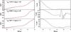 |
Fig. 2 Temperature structures for a MS, TO, and a RGB atmosphere as used in the present work (left panel). The black continuous line represents the model computed with the reference chemical mixture, the red dashed line the one assuming the CNONa1 mixture. In both cases, Y = 0.246. The right panel shows the percentage temperature difference between the two different chemical compositions. |
3.1. Producing the full chemical mixtures
The first step of our calculations was to provide the full chemical mixtures for the atmospheres. The three chemical compositions of Table 1 were derived from the stellar interior calculations and included only those elements relevant for that purpose in the form of mass fractions of metals normalized to unity. We will use the term “interior” throughout when speaking about this restricted set of elements.
While it is possible to consider only a subset of elements for the stellar interior modelling without adversely influencing the results, abundances for all remaining metals should be included in synthetic spectrum calculations. The fractions of elements in the interior mixture should then be converted into absolute abundances, including appropriate values for H and He, and the missing elements added. This process is essentially arbitrary, since there is no single way to fill in the missing metal abundances. We proceeded as follows:
-
the interior metal mixture, as listed in Table 1, wasconverted to a full metal mixture by filling in all the elementsexcept H and He. To do so, we tookas reference the chemical mixture of an α-enhanced,[Fe/H] = −1.5 model from the Castelli & Kurucz (2004) grid4. The total mass fraction of the elements considered for the interiors amounts to 0.986 in this mixture. Thus, their abundances in the interior mixtures of Table 1 were scaled by this factor, and the remaning 1.4% distributed over the missing elements according to their abundance fractions in the Castelli mixture. This has produced the three full metal mixtures of Table 2;
-
the helium mass fraction Y was set to the two possible values, Y = 0.246 or Y = 0.400.To produce a full set of abundances we then only needed to set a ratio between the H mass fraction X and the cumulative mass fraction of metals, Z. This was done by enforcing [Fe/H] = − 1.62. We came to such choice since observational evidence is that stars from different populations in GCs usually share the same [Fe/H] (see also the discussion in Sect. 2). The final full mixtures used for the atmospheres are listed in Table 2.
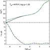 |
Fig. 3 Comparison of the temperature stratification for the four Teff = 4476 K, log g = 1.2 giant models (upper panel). The solid line denotes the reference mixture, the dashed line the CNONa mixture with Y = 0.246, the dot-dashed line the CNONa1 mixture with Y = 0.4, and the dash-dot-dot line the CNONa2 mixture. In the lower panel the percentage temperature difference for the last three mixtures with respect to the reference one is plotted; colour and line type are coded as in the upper panel. |
3.2. The model atmospheres
ATLAS 12 was employed to produce sets of model atmospheres from lower MS to bright RGB stars – the parameters are listed in Table 3 – for each of the four chemical compositions given in Table 2.
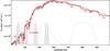 |
Fig. 4 Flux distribution for the RGB model with Teff = 4476 K and log g = 1.2 for the reference mixture (black) and the CNONa1 mixture (red), both with the standard helium content of Y = 0.246. We superimposed the transmission curves for the Johnson-Cousins U, B, V, and I filters (thin, black lines; left to right) and for the Strögren uvby filtes (grey-shaded regions). The synthetic spectra are broadened by convolution with a Gaussian of FWHM = 1700 km s-1 for readability purposes to roughly match the resolution of the Castelli & Kurucz (2004) ATLAS9-based fluxes. A number of molecular bands, which vary significantly between the two mixtures, are labelled by the name of the corresponding molecule. |
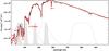 |
Fig. 6 As in Fig. 4 but now for the TO model with Teff = 4621 K and log g = 4.47. Here, the Na D doublet is also labelled. |
Figure 2 compares the temperature stratification in models employing the reference and CNONa1 (Y = 0.246) mixtures. Shown are the temperature (left panel) and the corresponding relative differences (right panel) against the Rosseland optical depth for three models corresponding to a cool MS, a TO, and an upper RGB star. Significant differences arise only in the outermost layers and only in cool models. As we will show below, these differences arise from the generally lower molecular absorption in the reference mixture compared to the other models, which mostly affects the outer layers of the cooler atmospheres. The strongest differences arise in the cool giants and are still appreciable in the coolest dwarf models, but become negligible in the warmer stars close to the TO or along the SGB. In the Teff = 4476 K giant, differences range from about 50 K at τross = 10-4 to about 250 K at τross = 10-6, which is the highest value encountered amongst the models explored in this work.
Figure 3 displays the temperature stratification of the RGB models shown in Fig. 2 for all our four mixtures as well as their deviations from the model calculated assuming the reference mixture. The results are representative of the general result for all models. Even large variations in the He abundance have a quite minor effect on the atmosphere structure (as is evident from the extremely similar structures in the CNONa1 Y = 0.246 and Y = 0.4 cases). We recall that this does not mean that the helium content will not affect the colours of second generation stars, since varying the He content has an important effect on the stellar interiors (Fig. 1). It merely indicates that the helium content does not affect these cool atmospheres, and thus the relationship between stellar parameters and colours. Passing from the CNONa1 to the CNONa2 mixture has a slightly more noticeable effect, but we stress that the difference never exceeds 25 K.
As far as the model atmospheres are concerned, one can thus conclude that the explored chemical mixtures do not have a major effect on the atmospheric structure, except in the outermost layers, where – at any rate – LTE models such as the ones employed here are less physically sound.
3.3. The synthetic spectra
We display in Figs. 4–6 the synthetic fluxes computed for the same three sets of parameters as in Fig. 2 as representative of the effects of changing chemical composition. More specifically, we display the reference case (black) and CNONa1 mixture (red), both with Y = 0.246. Synthetic spectra were computed with very fine sampling (Δλ/λ = 300 000) but are shown here after convolution with a FWHM = 1700 km s-1 Gaussian, for readibility purposes and to roughly match the resolution of Castelli & Kurucz (2004) fluxes. In each plot we label some prominent absorption features (mostly molecular bands), whose strength changes significantly among chemical mixtures.
Figure 4 compares the synthetic spectra of a Teff = 4476 K, log g = 1.2 giant. The CNONa1 mixture shows much stronger NH and CN absorption bands in the U, B, and I filters. This is essentially caused by the much higher N abundance of the CNONa1 mixture, despite the fact that the C abundance is lower. This indicates that the N abundance acts as bottleneck in forming CN molecules. Conversely, the G-band, a CH feature falling into the B filter appears stronger in the reference mixture, because the C abundance is higher. The increased opacity in the blue part of the spectrum for the CNONa1 mixture leads to the increase of the continuum flux redwards of about 450 nm, which explains the overall higher flux observed in the CNONa1 spectrum between 450 and 690 nm, and further in the red in the intervals along the strong CN absorption bands.
In the spectrum of the TO atmosphere (Teff = 6490 K, log g = 4.22, Fig. 5) the much higher temperature prevents the formation of CN and CH alike, thus removing the most prominent causes for increased blue opacity in the CNONa1 case as well as most of the influence of the G-band. Only the very strong NH band around 340 nm is still visible. The much more similar spectra for the two mixtures in the TO atmosphere are reflected in the extremely similar atmospheric structures displayed by the two TO models in Fig. 2.
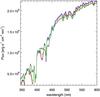 |
Fig. 7 Range between 300 and 600 nm is displayed for all mixtures considered, in the case of the Teff = 4476 K, log g = 1.2 giant atmosphere. Black line: reference mixture; red: CNONa1 (Y = 0.246); blue: CNONa1 (Y = 0.400); green: CNONa2 (Y = 0.246). |
The cool MS star (Teff = 4621 K, log g = 4.77, Fig. 6) displays features similar to the RGB one, but also shows a much stronger OH absorption at the blue edge of the U filter range in the reference case, owing to the higher O abundance: the same band is visible, but much less prominent, also in the MS and RGB stars. The Na D doublet becomes strongly wing-dominated in this spectrum and thusappears much stronger in the CNONa1 spectrum, where the Na abundancewas increased to reproduce the observed Na-O anticorrelation. Red CN bands have an almost negligible effect in this star. The strong absorption feature around 415 nm is the MgH A-X band.
In Fig. 7 we finally show how the blue-visible part of the spectrum changes among all four mixtures considered in the same RGB stellar model as described above. Two effects are immediately apparent: first, the CNONa2 mixture – sharing the same Z as the reference one as well as a lower N enhancement – shows less prominent NH and CN bands than the CNONa1 mixture as well as a continuum which closely resembles that of the reference mixture. Second, the change in the He abundance between the two CNONa1 mixture only has a tiny effect on the flux distribution. It has to be considered here that our choice of conserving [Fe/H] among mixtures leads to a lower Fe abundance (and Z, for that matter) in the CNONa1 mixture with Y = 0.400 with respect to the one with Y = 0.246, thus mitigating the main effect of increasing He, i.e. an increase in molecular weight.
We compared our synthetic fluxes with MARCS synthetic fluxes (Gustafsson et al. 2008), and obtained equivalent results for the reference composition. MARCS “CN-cycled” fluxes are produced with CNO abundances that depart less from the standard mixture than the ones we considered here, which, as expected, leads to a behaviour that is intermediate between our reference and CNONa1/2 cases.
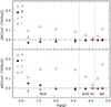 |
Fig. 8 Upper panel: difference between the UBVI bolometric corrections ΔBC for the reference mixture and the CNONa2 mixture with the same Y = 0.246. Bottom panel: as in the upper panel, but for the uvby system. |
4. Bolometric corrections and colour–magnitude-diagrams
As discussed in Sect. 2, we calculated the BC differences ΔBC for each of the key points in the UBVI and uvby photometric filters. We followed the method presented in Girardi et al. (2002) using passband definitions from Bessell (1990) and Strömgren (1956). The results for the different chemical compositions are displayed in Figs. 8–10. Figure 8 shows ΔBC for the CNONa2 mixture as a function of log g. As expected from the comparisons of the previous section, the U and u filters are the most affected by the different metal mixtures. The BC for the reference mixture is systematically higher by an amount that depends on the evolutionary phase. In both U and u bands ΔBC decreases moving from the low MS towards the TO (where it is practically negligible), then increases again along the RGB, reaching a local maximum around Teff = 4476 K and log g = 1.2, before decreasing slowly towards the tip of the RGB. Here, the highest values of ΔBC are of the order of 0.2 mag in u and 0.1 mag in U. The effect on the other filters is much smaller: the largest values of ΔBC are attained along the bright RGB and are of the order of 0.02–0.04 mag. Figure 9 displays the same comparison for the CNONa1 mixture, the mixture with enhanced C+N+O. The behaviour of ΔBC is qualitatively identical to the previous case, but the maximum values of ΔBC are increased. They are equal to ~0.30–0.35 mag in u, ~0.2 mag in U, ~0.1 mag in v and ~0.04 mag in the remaining filters. The final comparison among BCs is displayed in Fig. 10, which shows the differences between the CNONa1 mixture with Y = 0.246, and the same metal mixture with a much higher Y = 0.40.The values of ΔBC are reduced compared to varying the metal mixture. ΔBC is essentially zero in all filters from the low MS to the lower RGB, then becomes more and more negative while climbing the RGB. A higher helium abundance appears to increase the value of BC at low Teff and low gravities. The largest differences are obtained for the U and u bands, but are of the order of only 0.05 mag at most. These variations are small with respect to the effect of the metal mixture in U and u, but much more comparable for the other filters. Overall, the results of Fig. 10 are broadly consistent with the conclusions by Girardi et al. (2007), who studied the effect of enhanced He (for a scaled solar metal mixture) on the BCs for the UBVRIJHK filters.
Finally, we also investigated whether the values of ΔBC are affected by the choice of microturbulence, using the additional “test” calculations listed in Table 3. Microturbulence affects line absorption by reducing line saturation: the net effect is that saturated lines absorb more flux when microturbulence is higher, while unsaturated lines do not change. Because typical microturbulence values vary with the stellar evolutionary phases, one might need to take it into account in estimating ΔBC. In practice, we find that this effect is negligible: changing the value of Vturb from 2 km s-1 to 0.5 km s-1 changes the values of ΔBC by at most 0.01 mag.
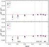 |
Fig. 10 As in Fig. 8, but for ΔBC calculated between the CNONa1 mixture with Y = 0.246 and the same metal mixture with Y = 0.400. |
Following the method outlined in Sect. 2 we then performed the first fully consistent theoretical study of the effect of the CNONa abundance anticorrelations on the MS-TO-RGB CMDs of Galactic GCs. In particular, we are now in the position to account for the CNONa pattern both in interior models and bolometric corrections.
Figures 11 to 15 display several CMDs in Johnson-Cousins as well as in Strömgren filters for the isochrones of Fig. 1. Given that the CNONa pattern we considered for the second generation stars is characterised by extreme values for the anticorrelation observed in Galactic GCs, the range of colours spanned by our isochrones should give a rough idea – considering also that the extension of the abundance anticorrelations varies from cluster to cluster (e.g. Carretta et al. 2010b) – of the maximum colour spread to be expected in the CMD of a generic Galactic GC.
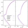 |
Fig. 11 Left: the MV-(B − V) CMD for the same isochrones as in Fig. 1. Different line-styles correspond to different element mixtures as labelled. Right: as on the left, but for the MV-(V − I) CMD. |
The commonly used BVI diagrams are shown in Fig. 11. The behaviour of the isochrones in these CMDs closely mirrors the HRD of Fig. 1, the reason being that in these filters the BCs are hardly affected by the change in the metal mixture and initial He content. As long as the sum of C+N+O is constant, second-generation stars are expected to overlap with first-generation objects. If the C+N+O is enhanced, only the TO and SGB regions are affected, whereas MS and RGB remain unchanged. An increase of Y shifts the MS (and to a lesser degree the RGB) towards bluer coloursbecause of hotter Teff in the evolutionary models.
The situation is – not unexpectedly – different when considering the UBV CMDs displayed in Fig. 12, given that U is the filter most affected by the change of the metal mixture owing to the emergence of strong molecular absorption in the atmosphere. In both diagrams the four isochrones are well separated along the various branches. Overall, our isochrone representative of second-generation stars with enhanced C+N+O is the reddest (dash-dotted line). Notice how second-generation stars born from a metal mixture with constant C+N+O (long-dashed line) follow a distinct sequence from the first-generation population (solid line), in spite of the fact that the HRDs of the underlying isochrones are identical. This is entirely owing to the effect of the metal mixture on the BCs.
The largest differences among the various isochrones appear along the RGB, where the mixture with anticorrelations causes redder (U − B) and (U − V) colours, at fixed MU. For example, at MU = 2.0 the RGBs representative of second-generation stars are redder by up to ~0.2 mag in (U − B) and ~0.3 mag in (U − V), depending on the metal mixture considered. We will compare this result with observational evidence in the discussion section.
It is also important to notice that an increase of Y up to 0.40 – a very extreme He-enhancement – shifts the isochrones of second-generation objects bluewards and thus closer again to the reference isochrone, contrasting the effect of CNONa variations which tend to shifts them redwards. The Y increase affects only the stellar interior models and may potentially even produce a bluer MS – depending on whether the anticorrelations are accompanied by a C+N+O enhancement or whether the C+N+O sum stays unchanged – especially in the U-(U − V) diagrams. The effect can best be seen by comparing the dot-dashed and dotted line in Fig. 12.
As for the Strömgren filters, the My-(u − y) and My-(v − y) CMDs are displayed in Fig. 13. The CMD with (v − y) colours show a behaviour very similar to the one seen in the V − (B − V) plane, except for the RGB. When the initial Y is kept constant, the bright RGB for the C+N+O enhanced mixture (dash-dotted line) is separated from the reference isochrone (solid) – at My = −2.0 the difference in (v − y) is ~0.2 mag – whereas the mixture with anticorrelations at constant C+N+O (long-dashed) does not modify the colour of the RGB. This difference in the behaviour of the RGB (v − y) colour for the two different mixtures with CNONa anticorrelations is essentially caused by the different BCs, rather than to the underlying isochrones.
Finally, the My-(u − y) CMD is similar qualitatively to the U-(U − B) diagram, with all different sequences well separated in the CMD when the initial He is kept constant.
Figure 14 displays the m1-(u − y) diagram, where the measured m1 = (v − b) − (b − y) in RGB stars is often used as an estimator of the cluster metallicity (see, e.g., Calamida et al. 2007, and references therein). Our comparison shows that the presence of CNONa anticorrelations produces a spread in the location of GC stars in this diagram. Focusing our attention on RGB stars only (the right part of the curves), the four different isochrones in Fig. 14 display quite different RGBs, which intersect at (u − y) around 2.6–2.8 mag. It is very interesting to notice that even for a constant C+N+O sum, [Fe/H], Y and total metallicity Z (the CNONa2 case; long-dashed line), the RGB representative of second-generation stars is different from the reference RGB, a clear effect of the difference in BCs.
Finally, we consider the behaviour of the index cy = c1 − (b − y), where c1 = (u − v) − (v − b) is found empirically to be sensitive to the N abundance (see, e.g., Yong et al. 2008). The cy index represents well c1, but removes much of the temperature sensitivity of this index. As a result, empirical V-cy diagrams of Galactic GCs display an almost vertical RGB at luminosities lower than the RGB bump (Yong et al. 2008). Figure 15 shows how this empirical behaviour is reproduced by the theoretical isochrones. The theoretical RGBs of the isochrones with our four selected chemical compositions are approximately vertical below the bump luminosity and are very well separated in cy colour. All isochrones representative of second-generation stars have redder cy colours, and the isochrone with the largest N abundance (at fixed Y – the dot-dashed isochrone for the CNONa1 mixture) is the reddest, in agreement with empirical results (Lind et al. 2011; Yong et al. 2008). Notice how in this diagram an increase of Y tends to move the RGBs of isochrones with CNONa anticorrelations further away from the reference isochrone (dotted line), despite the fact that the CNONa1 Y = 0.4 mixture has a lower N abundance than the CNONa1 Y = 0.246 mixture.
5. Discussion
Using ATLAS 12 model atmospheres and SYNTHE spectrosyntheses we calculated synthetic spectra for typical mixtures found in the various subpopulations of globular clusters. From the theoretical spectra we determined bolometric corrections for standard Johnson-Cousins and Strömgren filters, and finally predicted colours.
As a result of this work, we now have in hand complete and self-consistent theoretical predictions of the effect of abundance variations on observed CMDs, as they are found or discussed for the different globular cluster stellar generations. Globally, element abundance variations affect mainly the part of the spectra short of about 400 nm owing to changes in molecular bands. Therefore, colour changes are largest in the blue filters and their detection is easiest in the blue, independent of using broadband or narrow filters. Enhanced helium abundance is affecting only the interior structure of stars, leading to changes in luminosity and effective temperature, but is irrelevant for the atmospheric structure at fixed log g and Teff, even for Y as high as 0.400.
We did not investigate what the effect of CNO and He abundance would be in cluster with different [Fe/H]. While we do not expect the general behavior to change, the quantitative result is bound to be sensitive to the overall metal content of the cluster.
Using the combination of the previously computed isochrones and the new bolometric corrections for the different GC subpopulations, we summarize here the effects on the various possible colours in both Johnson-Cousins and Strömgren filter systems:
-
1.
BVI-diagrams:
-
a splitting5 of sequences along the MS up to theTO, and to a lesser degree of the RGB can only beachieved – within the element variationsdiscussed in this paper – byvarying the helium content Y. The CNONa anticorrelations influence neither the stellar models nor the spectrum sufficiently when the C+N+O-abundance is unchanged (mixture CNONa2 – Fig. 11);
-
on the other hand, a variation of the C+N+O-abundance (mixture CNONa1) leads to a split of the SGB; this is entirely an effect of the stellar models.
-
-
2.
UBV- and uy-diagrams: anticorrelations in CNONa abundances as well as Y-differences may lead to multiple sequences from the MS to the RGB, where the effect tends to be larger and may reach 0.2–0.3 mag. This multiplicity is independent of the sum of C+N+O (Fig. 12; left panel). The individual element variations are decisive. Helium enhancement, however, works in the opposite direction than CNONa anticorrelations (Fig. 13; left panel).
-
3.
vy-diagrams:
-
as for the BVI-colours, a splitting of the MS up to the TO can be achieved only by a variation in Y;
-
similarly, after the TO, a split of the SGB is the result of a change in C+N+O;
-
additionally, a split along the RGB may result both from helium and from C+N+O variations; this is different from the BVI-case (Fig. 13; right panel).
-
-
4.
m1uy-diagrams:
-
CNONa anticorrelations lead to splits along the MS;
-
along the SG and RGB the same anticorrelations but helium variations lead to colour differences as well;
-
the sign of the colour change is different for the lower and upper part of the RGB (Fig. 14).
-
-
5.
cyV-diagrams: here, all parts of a CMD show the influence of both element anticorrelations and of helium variations, and a strong separation can be seen (Fig. 15).
Our calculations also enable us to briefly address the question raised by the photometric observations by Lee et al. (2009), who find broad distributions of the hk index – defined as hk = (Ca − b)-(b − y) – in RGB sequences of several Galactic GCs; they determined a broadening of the order of ~0.2 mag in hk at fixed V magnitude and attribute this to a spread in calcium abundance, given that the hk index is sensitive to the ionized calcium H and K lines. On the other hand, direct spectroscopic measurements of calcium abundance by Carretta et al. (2010a) do not find any significant spread in individual clusters. We tested with our spectra whether the CNONa abundance anticorrelations affect the hk index at our chosen RGB key points. For this purpose we calculated differences in the hk index among our adopted chemical compositions employing the appropriate profile from the Ca filter taken from the Asiago photometric database (Fiorucci & Munari 2003). We find an effect of at most only ~ 0.04 mag in the hk colour at fixed MV, second-generation stars being systematically bluer. Therefore, CNONa anticorrelations cannot fully explain hk-variations of 0.2 mag.
In comparison with observations we find that our MV − cy-diagram closely follows the empirical results by Yong et al. (2008) and Lind et al. (2011), which adds support to our theoretical models. We thereby also confirm that this index is well suited to investigate photometrically variations of nitrogen abundance along the lower RGB.
Also the U-(U − B) CMD of Fig. 12 interestingly agrees with the results by Marino et al. (2008) about M 4 RGB stars. These authors have found that in the U-(U − B) CMD, objects with high Na – represented by our isochrones for the two compositions with CNONa anticorrelations – are distributed to the red of stars with low Na – represented by our isochrone with the reference chemical composition.
A further interesting case is given by NGC 6752. In Sect. 1 we already mentioned that Milone et al. (2010b) report about an MS splitting in visual HST filters, and an RGB split in a UB-CMD. The SGB appears to be single in the visual. Yong et al. (2008) found a variation in nitrogen abundance of up to 1.95 dex, correlating with the c1 index. Recently, Kravtsov et al. (2011) claimed a splitting of the SGB in the U vs. B − I diagram, and a broadening of the RGB in the U vs. U − B plane. The single SGB in B − I is indicative of a constant C+N+O, the MS splitting of He-enhancement in the second generation stars, and the broadening of the RGB in blue filters agrees with both. In conclusion, if these findings are confirmed, they would indicate a subpopulation of CNONa2 type, but with enhanced helium.
Finally, we comment on the case of NGC 1851 which was observed in different bands. The y-(v-y), y-(b-y), and m1-(u-y) CMDs by Calamida et al. (2007) show a spread, if not a bimodality, along the RGB. TheHST mF606W-(mF606W − mF814W) diagram by Milone et al. (2008), approximately equivalent to our MV vs. V − I CMD, displays a double SGB, but no other splitting.In the UBVI observations of Han et al. (2009), finally, no RGB split is observed in the MV vs. V − I CMD, while it is quite evident in the MU vs. (U − I) one (see Han et al. 2009, Fig. 1). It has to be noted that Han et al. (2009) could not detect any SGB split in the MV vs. V − I CMD, probably owing to the lower quality of their ground-based photometry compared to the HST-based one in Milone et al. (2008). On the basis of our results, only a second-generation population with enhanced C+N+O and “normal” He can satisfy all these constraints. Indeed, a second generation with constant C+N+O will not produce a spread along the RGB in the vy CMD, and a He enhancement would reveal itself along the MS of the mF606W-(mF606W − mF814W) CMD. Also the synthetic HB simulations by Salaris et al. (2008) seem to exclude a He variation among the cluster subpopulations.
In summary, we are now able to investigate in detail clusters with known or suspected abundance variations and several subpopulations, using information from their CMDs,on the basis of fully self-consistent interior and atmosphere models. As a first application, in a following paper we will analyse in detail the cluster NGC 1851 with more specific calculations.
Online material
Appendix A:
Abundances for all elements in the considered mixtures.
The BaSTI database is available at http:/www.oa-teramo.inaf.it/BASTI.
We did not include TiO lines in the calculations after verifying that no significant TiO bands formed in some representative cases, given that they would have made the calculations remarkably longer.
The synthetic fluxes are made available through CDS, the atmosphere models can be obtained by request to the authors.
Available online at http://wwwuser.oat.ts.astro.it/castelli/grids.html
In real globular clusters the splitting may in fact appear as a spread, depending on the nature of the element abundance variations.
Acknowledgments
L.S. warmly acknowledges F. Castelli for her prompt help with a number of ATLAS12-related problems, as well as A. F. Marino for a number of comments and useful discussions of the paper findings. M.S. is grateful to the Max Planck Institute for Astrophysics for their hospitality and support. A.W. received financial support from the Excellence cluster “Origin and Structure of the Universe” (Garching). S.C. acknowledges the financial support of INAF through the PRIN INAF 2009 (P.I.: R. Gratton).
References
- Anderson, J. 1998, Ph.D. Thesis, Univ. California, Berkeley [Google Scholar]
- Anderson, J., Piotto, G., King, I. R., Bedin, L. R., & Guhathakurta, P. 2009, ApJ, 697, L58 [NASA ADS] [CrossRef] [Google Scholar]
- Bedin, L. R., Piotto, G., Anderson, J., et al. 2004, ApJ, 605, L125 [NASA ADS] [CrossRef] [Google Scholar]
- Bellini, A., Bedin, L. R., Piotto, G., et al. 2010, AJ, 140, 631 [NASA ADS] [CrossRef] [Google Scholar]
- Bessell, M. S. 1990, PASP, 102, 1181 [NASA ADS] [CrossRef] [Google Scholar]
- Bonifacio, P., Pasquini, L., Molaro, P., et al. 2007, A&A, 470, 153 [NASA ADS] [CrossRef] [EDP Sciences] [Google Scholar]
- Bragaglia, A., Carretta, E., Gratton, R., et al. 2010, A&A, 519, A60 [NASA ADS] [CrossRef] [EDP Sciences] [Google Scholar]
- Calamida, A., Bono, G., Stetson, P. B., et al. 2007, ApJ, 670, 400 [NASA ADS] [CrossRef] [Google Scholar]
- Carretta, E., Gratton, R. G., Lucatello, S., Bragaglia, A., & Bonifacio, P. 2005, A&A, 433, 597 [NASA ADS] [CrossRef] [EDP Sciences] [Google Scholar]
- Carretta, E., Bragaglia, A., Gratton, R. G., et al. 2009, A&A, 505, 117 [NASA ADS] [CrossRef] [EDP Sciences] [Google Scholar]
- Carretta, E., Bragaglia, A., Gratton, R., et al. 2010a, ApJ, 712, L21 [NASA ADS] [CrossRef] [Google Scholar]
- Carretta, E., Bragaglia, A., Gratton, R., et al. 2010b, A&A, 516, A55 [NASA ADS] [CrossRef] [EDP Sciences] [Google Scholar]
- Cassisi, S., Salaris, M., Castelli, F., & Pietrinferni, A. 2004, ApJ, 616, 498 [NASA ADS] [CrossRef] [Google Scholar]
- Cassisi, S., Salaris, M., Pietrinferni, A., et al. 2008, ApJ, 672, L115 [NASA ADS] [CrossRef] [Google Scholar]
- Castelli, F. 2005, Mem. Soc. Astron. Ital., Supp. 8, 25 [Google Scholar]
- Castelli, F., & Kurucz, R. L. 2004 [arXiv:astro-ph/0405087] [Google Scholar]
- Cohen, J. G. 1978, ApJ, 223, 487 [NASA ADS] [CrossRef] [Google Scholar]
- Da Costa, G. S., Held, E. V., Saviane, I., & Gullieuszik, M. 2009, ApJ, 705, 1481 [NASA ADS] [CrossRef] [Google Scholar]
- D’Antona, F., Bellazzini, M., Caloi, V., et al. 2005, ApJ, 631, 868 [NASA ADS] [CrossRef] [Google Scholar]
- Dotter, A., Chaboyer, B., Ferguson, J. W., et al. 2007, ApJ, 666, 403 [NASA ADS] [CrossRef] [Google Scholar]
- Fiorucci, M., & Munari, U. 2003, A&A, 401, 781 [NASA ADS] [CrossRef] [EDP Sciences] [Google Scholar]
- Girardi, L., Bertelli, G., Bressan, A., et al. 2002, A&A, 391, 195 [NASA ADS] [CrossRef] [EDP Sciences] [Google Scholar]
- Girardi, L., Castelli, F., Bertelli, G., & Nasi, E. 2007, A&A, 468, 657 [NASA ADS] [CrossRef] [EDP Sciences] [Google Scholar]
- Gratton, R., Sneden, C., & Carretta, E. 2004, ARA&A, 42, 385 [NASA ADS] [CrossRef] [Google Scholar]
- Gustafsson, B., Edvardsson, B., Eriksson, K., et al. 2008, A&A, 486, 951 [NASA ADS] [CrossRef] [EDP Sciences] [Google Scholar]
- Han, S.-I., Lee, Y.-W., Joo, S.-J., et al. 2009, ApJ, 707, L190 [NASA ADS] [CrossRef] [Google Scholar]
- Johnson, C. I., Pilachowski, C. A., Michael Rich, R., & Fulbright, J. P. 2009, ApJ, 698, 2048 [NASA ADS] [CrossRef] [Google Scholar]
- Kravtsov, V., Alcaíno, G., Marconi, G., & Alvarado, F. 2010a, A&A, 512, L6 [NASA ADS] [CrossRef] [EDP Sciences] [Google Scholar]
- Kravtsov, V., Alcaíno, G., Marconi, G., & Alvarado, F. 2010b, A&A, 516, A23 [NASA ADS] [CrossRef] [EDP Sciences] [Google Scholar]
- Kravtsov, V., Alcaino, G., Marconi, G., & Alvarado, F. 2011, A&A, 527, L9 [NASA ADS] [CrossRef] [EDP Sciences] [Google Scholar]
- Kurucz, R. L. 2005a, Mem. Soc. Astron. Ital. Supp., 8, 14 [Google Scholar]
- Kurucz, R. L.2005b, Mem. Soc. Astron. Ital. Supp., 8, 86 [Google Scholar]
- Lee, J., Kang, Y., Lee, J., & Lee, Y. 2009, Nature, 462, 480 [NASA ADS] [CrossRef] [PubMed] [Google Scholar]
- Lee, Y., Joo, S., Han, S., et al. 2005, ApJ, 621, L57 [NASA ADS] [CrossRef] [Google Scholar]
- Lee, Y.-W., Joo, J.-M., Sohn, Y.-J., et al. 1999, Nature, 402, 55 [NASA ADS] [CrossRef] [Google Scholar]
- Lind, K., Primas, F., Charbonnel, C., Grundahl, F., & Asplund, M. 2009, A&A, 503, 545 [NASA ADS] [CrossRef] [EDP Sciences] [MathSciNet] [Google Scholar]
- Lind, K., Charbonnel, C., Decressin, T., et al. 2011, A&A, 527, A148 [NASA ADS] [CrossRef] [EDP Sciences] [Google Scholar]
- Marino, A. F., Villanova, S., Piotto, G., et al. 2008, A&A, 490, 625 [NASA ADS] [CrossRef] [EDP Sciences] [Google Scholar]
- Marino, A. F., Milone, A. P., Piotto, G., et al. 2009, A&A, 505, 1099 [NASA ADS] [CrossRef] [EDP Sciences] [Google Scholar]
- Milone, A. P., Bedin, L. R., Piotto, G., et al. 2008, ApJ, 673, 241 [NASA ADS] [CrossRef] [Google Scholar]
- Milone, A. P., Piotto, G., Bedin, L. R., et al. 2010a, in SF2A-2010: Proceedings of the Annual meeting of the French Society of Astronomy and Astrophysics, ed. S. Boissier, M. Heydari-Malayeri, R. Samadi, D. Valls-Gabaud, 319 [Google Scholar]
- Milone, A. P., Piotto, G., King, I. R., et al. 2010b, ApJ, 709, 1183 [NASA ADS] [CrossRef] [Google Scholar]
- Norris, J. E. 2004, ApJ, 612, L25 [NASA ADS] [CrossRef] [Google Scholar]
- Pasquini, L., Bonifacio, P., Molaro, P., et al. 2005, A&A, 441, 549 [NASA ADS] [CrossRef] [EDP Sciences] [Google Scholar]
- Pietrinferni, A., Cassisi, S., Salaris, M., & Castelli, F. 2006, ApJ, 642, 797 [NASA ADS] [CrossRef] [Google Scholar]
- Pietrinferni, A., Cassisi, S., Salaris, M., Percival, S., & Ferguson, J. W. 2009, ApJ, 697, 275 [NASA ADS] [CrossRef] [Google Scholar]
- Piotto, G. 2008, in IAU Symp. 246, ed. E. Vesperini, M. Giersz, & A. Sills, 141 [Google Scholar]
- Piotto, G., Villanova, S., Bedin, L. R., et al. 2005, ApJ, 621, 777 [NASA ADS] [CrossRef] [Google Scholar]
- Piotto, G., Bedin, L. R., Anderson, J., et al. 2007, ApJ, 661, L53 [NASA ADS] [CrossRef] [Google Scholar]
- Renzini, A. 2008, MNRAS, 391, 354 [NASA ADS] [CrossRef] [Google Scholar]
- Salaris, M., Weiss, A., Ferguson, J. W., & Fusilier, D. J. 2006, ApJ, 645, 1131 [NASA ADS] [CrossRef] [Google Scholar]
- Salaris, M., Cassisi, S., & Pietrinferni, A. 2008, ApJ, 678, L25 [NASA ADS] [CrossRef] [Google Scholar]
- Sbordone, L. 2005, Mem. Soc. Astron. Ital. Supp., 8, 61 [Google Scholar]
- Sbordone, L., Bonifacio, P., & Castelli, F. 2007, in IAU Symp. 239, ed. T. Kuroda, H. Sugama, R. Kanno, & M. Okamoto, 71 [Google Scholar]
- Sbordone, L., Limongi, M., Chieffi, A., et al. 2009, A&A, 503, 121 [NASA ADS] [CrossRef] [EDP Sciences] [Google Scholar]
- Shen, Z., Bonifacio, P., Pasquini, L., & Zaggia, S. 2010, A&A, 524, L2 [NASA ADS] [CrossRef] [EDP Sciences] [Google Scholar]
- Sollima, A., Pancino, E., Ferraro, F. R., et al. 2005, ApJ, 634, 332 [NASA ADS] [CrossRef] [Google Scholar]
- Strömgren, B. 1956, Vistas in Astronomy, 2, 1336 [Google Scholar]
- Ventura, P., Caloi, V., D’Antona, F., et al. 2009, MNRAS, 399, 934 [NASA ADS] [CrossRef] [Google Scholar]
- Villanova, S., Piotto, G., King, I. R., et al. 2007, ApJ, 663, 296 [NASA ADS] [CrossRef] [Google Scholar]
- Villanova, S., Geisler, D., & Piotto, G. 2010, ApJ, 722, L18 [NASA ADS] [CrossRef] [Google Scholar]
- Yong, D., Grundahl, F., D’Antona, F., et al. 2009, ApJ, 695, L62 [NASA ADS] [CrossRef] [Google Scholar]
- Yong, D., Grundahl, F., Johnson, J. A., & Asplund, M. 2008, ApJ, 684, 1159 [NASA ADS] [CrossRef] [Google Scholar]
All Tables
Mass and number fractions (normalized to unity) for the three metal mixtures considered.
Abundances for selected elements in the four chemical mixtures used for the atmosphere computations.
All Figures
|
Fig. 1 Theoretical isochrones from the MS to the tip of the RGB for the four different chemical compositions. The solid line corresponds to both the reference first-generation population and the second-generation population with the CNONa2 metal mixture (both with Y = 0.246), because they are virtually identical. The black dots along this isochrone denote the points for which we calculated the model atmosphere and synthetic spectra. The dashed line corresponds to the second- generation population with the CNONa1 metal mixture (Y = 0.246), while the dash-dotted line is for the same population, but for an initial He mass fraction of Y = 0.40.(See the text for more details.) |
| In the text | |
|
Fig. 2 Temperature structures for a MS, TO, and a RGB atmosphere as used in the present work (left panel). The black continuous line represents the model computed with the reference chemical mixture, the red dashed line the one assuming the CNONa1 mixture. In both cases, Y = 0.246. The right panel shows the percentage temperature difference between the two different chemical compositions. |
| In the text | |
|
Fig. 3 Comparison of the temperature stratification for the four Teff = 4476 K, log g = 1.2 giant models (upper panel). The solid line denotes the reference mixture, the dashed line the CNONa mixture with Y = 0.246, the dot-dashed line the CNONa1 mixture with Y = 0.4, and the dash-dot-dot line the CNONa2 mixture. In the lower panel the percentage temperature difference for the last three mixtures with respect to the reference one is plotted; colour and line type are coded as in the upper panel. |
| In the text | |
|
Fig. 4 Flux distribution for the RGB model with Teff = 4476 K and log g = 1.2 for the reference mixture (black) and the CNONa1 mixture (red), both with the standard helium content of Y = 0.246. We superimposed the transmission curves for the Johnson-Cousins U, B, V, and I filters (thin, black lines; left to right) and for the Strögren uvby filtes (grey-shaded regions). The synthetic spectra are broadened by convolution with a Gaussian of FWHM = 1700 km s-1 for readability purposes to roughly match the resolution of the Castelli & Kurucz (2004) ATLAS9-based fluxes. A number of molecular bands, which vary significantly between the two mixtures, are labelled by the name of the corresponding molecule. |
| In the text | |
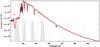 |
Fig. 5 As in Fig. 4 but now for the TO model with Teff = 6490 K and log g = 4.22. |
| In the text | |
|
Fig. 6 As in Fig. 4 but now for the TO model with Teff = 4621 K and log g = 4.47. Here, the Na D doublet is also labelled. |
| In the text | |
|
Fig. 7 Range between 300 and 600 nm is displayed for all mixtures considered, in the case of the Teff = 4476 K, log g = 1.2 giant atmosphere. Black line: reference mixture; red: CNONa1 (Y = 0.246); blue: CNONa1 (Y = 0.400); green: CNONa2 (Y = 0.246). |
| In the text | |
|
Fig. 8 Upper panel: difference between the UBVI bolometric corrections ΔBC for the reference mixture and the CNONa2 mixture with the same Y = 0.246. Bottom panel: as in the upper panel, but for the uvby system. |
| In the text | |
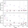 |
Fig. 9 As in Fig. 8 but for the CNONa1 mixture. |
| In the text | |
|
Fig. 10 As in Fig. 8, but for ΔBC calculated between the CNONa1 mixture with Y = 0.246 and the same metal mixture with Y = 0.400. |
| In the text | |
|
Fig. 11 Left: the MV-(B − V) CMD for the same isochrones as in Fig. 1. Different line-styles correspond to different element mixtures as labelled. Right: as on the left, but for the MV-(V − I) CMD. |
| In the text | |
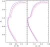 |
Fig. 12 As in Fig. 11 but for the MU-(U − B) and MU-(U − V) CMDs. |
| In the text | |
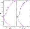 |
Fig. 13 As in Fig. 11 but for the My-(v − y) and My-(u − y) CMDs. |
| In the text | |
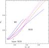 |
Fig. 14 As in Fig. 11 but for the m1-(u − y) CMD. |
| In the text | |
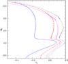 |
Fig. 15 As in Fig. 11 but for the MV-(cy) CMD. |
| In the text | |
Current usage metrics show cumulative count of Article Views (full-text article views including HTML views, PDF and ePub downloads, according to the available data) and Abstracts Views on Vision4Press platform.
Data correspond to usage on the plateform after 2015. The current usage metrics is available 48-96 hours after online publication and is updated daily on week days.
Initial download of the metrics may take a while.