| Issue |
A&A
Volume 534, October 2011
|
|
|---|---|---|
| Article Number | A51 | |
| Number of page(s) | 16 | |
| Section | Cosmology (including clusters of galaxies) | |
| DOI | https://doi.org/10.1051/0004-6361/201015893 | |
| Published online | 30 September 2011 | |
Measuring the integrated Sachs-Wolfe effect
1
Laboratoire AIM, UMR CEA-CNRS-Paris 7, Irfu, SAp/SEDI, Service d’Astrophysique, CEA Saclay, 91191 Gif-sur-Yvette Cedex, France
e-mail: francois-xavier.dupe@cea.fr; anais.rassat@cea.fr
2
GREYC UMR CNRS 6072, Université de Caen Basse-Normandie/ENSICAEN, 6 Bd Maréchal Juin, 14050 Caen, France
Received: 8 October 2010
Accepted: 13 June 2011
Context. One of the main challenges of modern cosmology is to understand the nature of the mysterious dark energy that causes the cosmic acceleration. The integrated Sachs-Wolfe (ISW) effect is sensitive to dark energy, and if detected in a universe where modified gravity and curvature are excluded, presents an independent signature of dark energy. The ISW effect occurs on large scales where cosmic variance is high and where owing to the Galactic confusion we lack large amounts of data in the CMB as well as large-scale structure maps. Moreover, existing methods in the literature often make strong assumptions about the statistics of the underlying fields or estimators. Together these effects can severely limit signal extraction.
Aims. We aim to define an optimal statistical method for detecting the ISW effect that can handle large areas of missing data and minimise the number of underlying assumptions made about the data and estimators.
Methods. We first review current detections (and non-detections) of the ISW effect, comparing statistical subtleties between existing methods, and identifying several limitations. We propose a novel method to detect and measure the ISW signal. This method assumes only that the primordial CMB field is Gaussian. It is based on a sparse inpainting method to reconstruct missing data and uses a bootstrap technique to avoid assumptions about the statistics of the estimator. It is a complete method, which uses three complementary statistical methods.
Results. We apply our method to Euclid-like simulations and show we can expect a ~7σ model-independent detection of the ISW signal with WMAP7-like data, even when considering missing data. Other tests return ~5σ detection levels for a Euclid-like survey. We find that detection levels are independent from whether the galaxy field is normally or lognormally distributed. We apply our method to the 2 Micron All Sky Survey (2MASS) and WMAP7 CMB data and find detections in the 1.0−1.2σ range, as expected from our simulations. As a by-product, we have also reconstructed the full-sky temperature ISW field from the 2MASS data.
Conclusions. We present a novel technique based on sparse inpainting and bootstrapping, which accurately detects and reconstructs the ISW effect.
Key words: methods: data analysis / cosmic background radiation / large-scale structure of Universe / dark energy / dark matter / methods: statistical
© ESO, 2011
1. Introduction
The recent abundance of cosmological data in the last few decades (for an example of the most recent results see Komatsu et al. 2009; Percival et al. 2007a; Schrabback et al. 2010) has provided compelling evidence towards a standard concordance cosmology, in which the Universe is composed of approximately 4% baryons, 22% “dark” matter and 74% “dark” energy.
One of the main challenges of modern cosmology is to understand the nature of the mysterious dark energy that drives the observed cosmic acceleration (Albrecht et al. 2006; Peacock et al. 2006).
The integrated Sachs-Wolfe (ISW) (Sachs & Wolfe 1967) effect is a secondary anisotropy of the cosmic microwave background (CMB), which arises because of the variation with time of the cosmic gravitational potential between local observers and the surface of last scattering. The potential can be traced by large-scale structure (LSS) surveys (Crittenden & Turok 1996), and the ISW effect is therefore a probe that links the high-redshift CMB with the low-redshift matter distribution and can be detected by cross-correlating the two.
As a cosmological probe, the ISW effect has less statistical power than weak lensing or galaxy clustering (see, e.g., Refregier et al. 2010), but it is directly sensitive to dark energy, curvature or modified gravity (Kamionkowski & Spergel 1994; Kinkhabwala & Kamionkowski 1999; Carroll et al. 2005; Song et al. 2007), such that in universes where modified gravity and curvature are excluded, detection of the ISW signal provides a direct signature of dark energy. In more general universes, the ISW effect can be used to trace alternative models of gravity.
The CMB WMAP survey is already optimal for detecting the ISW signal (see Sects. 2 and 3), and significance is not expected to increase with the arrival of Planck, unless the effect of the foreground Galactic mask can be reduced. However the amplitude of the measured ISW signal should depend strongly on the details of the local tracer of mass. Survey optimisations (Douspis et al. 2008) show that an ideal ISW survey requires the same configuration as surveys that are optimised for weak-lensing or galaxy clustering-meaning that an optimal measure of the ISW signal will essentially come “for free” with future planned weak-lensing and galaxy clustering surveys (see, e.g., the Euclid survey Refregier et al. 2010). In the best scenario, a 4σ detection is expected (Douspis et al. 2008), and it has been shown that combined with weak lensing, galaxy correlation and other probes such as clusters, the ISW can be useful to break parameter degeneracies (Refregier et al. 2010), making it a promising probe.
Initial attempts to detect the ISW effect with COBE as the CMB tracer were fruitless (Boughn & Crittenden 2002), but since the arrival of WMAP data, tens of positive detections have been made, with the highest significance reported for analyses using a tomographic combination of surveys (see Sects. 2 and 3, for a detailed review of detections). However, several studies using the same tracer of LSS appear to have contradicting conclusions, some analyses do not find correlation where others do, and as statistical methods for analysing the data evolve, the significance of the ISW signal is sometimes reduced (see, e.g., Afshordi et al. 2004; Rassat et al. 2007; Francis & Peacock 2010b).
In Sect. 2 we describe the cause of the ISW effect and review current detections. In Sect. 3 we describe the methodology for detecting and measuring the ISW signal, and review a large portion of reported detections in the literature as well as their advantages and disadvantages. After identifying the main problems with current methods, we propose a new and complete method in Sect. 4, which capitalises on the fact that different statistical methods are complementary. It also uses sparse inpainting to solve the problem of missing data and a bootstrapping technique to measure the estimator’s probability distribution function (PDF). In Sect. 5 we validate our new method using simulations for 2MASS and Euclid-like surveys. In Sect. 6 we apply our new method to WMAP 7 and the 2MASS survey. In Sect. 7 we present our conclusions.
2. The integrated Sachs-Wolfe effect
2.1. Origin of the integrated Sachs-Wolfe effect
General relativity predicts that the wavelength of electromagnetic radiation is sensitive to gravitational potentials, an effect that is called gravitational redshift. Photons travelling from the surface of last scattering will necessarily travel through the gravitational potential of LSSs on their way to the observer; these will be blueshifted as they enter the potential well and redshifted as they exit the potential. These shifts will accumulate along the line of sight of the observer. The total shift in wavelength will translate into a change in the measured temperature-temperature anisotropy of the CMB, and can be calculated by  (1)where \begin{formule}$T$\end{formule} is the temperature of the CMB, η is the conformal time, defined by
  and η0 and ηL represent the conformal times today and at the surface of the last scattering respectively. The unit vector
  is along the line of sight and the gravitational potential Φ(x,η) depends on position and time. The integral depends on the rate of change of the potential Φ′ = dΦ/dη.
In a universe with no dark energy or curvature, the cosmic (linear) gravitational potential does not vary with time, so that blue and redshift will always cancel out because Φ′ = 0 and there will be no net effect on the wavelength of the photon.
However, if there is dark energy or curvature (Sachs & Wolfe 1967; Kamionkowski & Spergel 1994; Kinkhabwala & Kamionkowski 1999), the right hand side of Eq. (1) will be non-null as the cosmic potential will change with time (see, e.g., Dodelson 2003), resulting in a secondary anisotropy in the CMB temperature field.
Meta-analysis of ISW detections to date and their reported statistical significance.
2.2. Detection of the ISW signal
The ISW effect leads to a linear scale secondary anisotropy in the temperature field of the CMB, and will thus affect the CMB temperature power spectrum at large scales. Because of the primordial anisotropies and cosmic variance on large scales, the ISW signal is difficult to detect directly in the temperature map of the CMB, but Crittenden & Turok (1996) showed it could be detected through cross-correlation of the CMB with a local tracer of mass.
The first attempt to detect the ISW effect (Boughn & Crittenden 2002) involved correlating the CMB explorer data (Bennett et al. 1990, COBE) with XRB (Boldt 1987) and NVSS data (Condon et al. 1998). This analysis did not find a significant correlation between the local tracers of mass and the CMB. Since the release of data from the Wilkinson Microwave Anisotropy Probe (Spergel et al. 2003, WMAP), more than 20 studies (see Table 1) have investigated cross-correlations between the different years of WMAP data and local tracers selected using various wavelengths: X-ray (Boldt 1987, XRB survey); optical (Agüeros et al. 2006; Adelman-McCarthy et al. 2008, SDSS galaxies), (Anderson et al. 2001, SDSS QSOs), (Doroshkevich et al. 2004, SDSS LRGs), (Maddox et al. 1990, APM); near infrared (Jarrett et al. 2000, 2MASS); radio (Condon et al. 1998, NVSS).
The full sky WMAP data have sufficient resolution on large scales that the measure of the ISW signal is cosmic variance limited. The best LSS probe of the ISW effect should include maximum sky coverage and full redshift coverage of the dark-energy-dominated era (Douspis et al. 2008). No such survey yet exists, so there is room for improvement on the ISW detection as larger and larger LSS surveys arise. For this reason, we classify the current ISW detections according to their tracer of LSS, and not to the CMB map used.
The ISW signal can be measured using various statistical spaces; we classify detections in Table 1 into three measurement “domains”: D1 corresponds to the spherical harmonic space; D2 to the configuration space and D3 to the wavelet space. (In Sect. 3 we review the different methods for quantifying the statistical significance of each measurement.)
There are only two analyses that use COBE as CMB data (with XRB and NVSS data, Boughn & Crittenden 2002), and both report null detections, which is probably caused by the low angular resolution of COBE even at large scales. The rest are processed correlating WMAP data from years 1, 3, and 5 (respectively “W1”, “W3”, and “W5” in Table 1).
Most ISW detections reported in Table 1 are relatively “weak” (<3σ), which is expected from theory for a concordance cosmology. Higher detections are reported for the NVSS survey (Pietrobon et al. 2006; McEwen et al. 2008; Giannantonio et al. 2008), though weak and marginal detections using NVSS data are also reported (Hernández-Monteagudo 2010; Sawangwit et al. 2010). High detections are often made using a wavelet analysis (Pietrobon et al. 2006; McEwen et al. 2008), though a similar study by McEwen et al. (2007) using the same data but a different analysis method finds a weaker signal. The highest detection is reported using a tomographic combination of all surveys (XRB, SDSS galaxies, SDSS QSOs, 2MASS and NVSS, Giannantonio et al. 2008), as expected given the larger redshift coverage of the analysis.
Several analyses have been revisited to seek confirmation of previous detections. In some cases, results are very similar (Padmanabhan et al. 2005; Granett et al. 2009; Giannantonio et al. 2008, for SDSS LRGs; Giannantonio et al. 2006, 2008 for SDSS Quasars; Afshordi et al. 2004; Rassat et al. 2007, for 2MASS), but in some cases they are controversially different (e.g., Pietrobon et al. 2006 and Sawangwit et al. 2010 for NVSS or; Afshordi et al. 2004 and; Giannantonio et al. 2008 for 2MASS).
We also notice that as certain surveys are revisited, there is a trend for the statistical significance to be reduced, e.g., detections from 2MASS decrease from a 2.5σ detection (Afshordi et al. 2004), to 2σ (Rassat et al. 2007), to 0.5σ (Giannantonio et al. 2008) to “weak” (Francis & Peacock 2010b). Detections using SDSS LRGs decrease from 2.5σ (Padmanabhan et al. 2005), to 2–2.2σ (Granett et al. 2009; Giannantonio et al. 2008), to “marginal” (Sawangwit et al. 2010). Furthermore, there tends to be a “sociological bias” in the interpretation of the confidence on the signal detection. The first detections interpret a 2–3σ detection as “tentative” (Boughn & Crittenden 2004, 2005), while other studies with a similar detection level report “independent evidence of dark energy” (Afshordi et al. 2004; Gaztañaga et al. 2006).
Review of advantages and disadvantages of measuring spectra vs. fields to infer an ISW detection (top). Review of statistical methods in the literature and their respective advantages and disadvantages (bottom).
3. Methodology for detecting the ISW effect
We are interested in qualifying the differences between different statistical methods that exist in the literature and in comparing them with a new method we present in Sect. 4. By statistical method we mean the method that is used to quantify the significance of a signal, not the space in which the signal is measured. Therefore, and without loss of generality, the review presented in Sect. 3.2 summarises methods using spherical harmonics. We compare the pros and cons of each method in Sect. 3.3. We begin by describing how the ISW signal can be measured in spherical harmonics in Sect. 3.1
3.1. ISW signal in spherical harmonics
In general, any field can be decomposed by a series of functions that form an orthonormal set, as do the spherical harmonic functions Yℓm(θ,φ). Therefore, a projected galaxy overdensity (δg) or temperature anisotropy (δT) field δX(θ,φ), where X = g,T, can be decomposed into  (2)where
  are the spherical harmonic coefficients of the field. The two-point galaxy-temperature cross-correlation function can then be written
 ![\begin{equation} C_{\rm gT}(\ell)=\frac{1}{(2\ell+1)}\sum_m \mathcal{R} e\left[a^g_{\ell m} (a^{T}_{\ell m})^*\right], \end{equation}](/articles/aa/full_html/2011/10/aa15893-10/aa15893-10-eq28.png) (3)where taking the real part of the product ensures that CgT(ℓ) = CTg(ℓ).
(3)where taking the real part of the product ensures that CgT(ℓ) = CTg(ℓ).
The theory for the angular cross-correlation function is given by 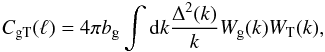 (4)where
 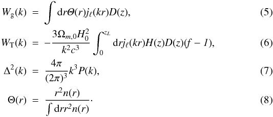 In these equations, r represents the co-moving distance, zL the redshift at the last scattering surface, k the Fourier mode wavenumber and quantities that depend on the redshift z have an intrinsic dependence on r: H(z) = H(z(r)). The function f is the linear growth factor given by
  , where D(z) is the linear growth that measures the growth of structure. The cross-correlation function depends on the survey selection function given by n(r) in units of galaxies per unit volume. The quantities Ωm,0 and H0 are the values of the matter density and the Hubble parameter at z = 0. Units are chosen so that the quantity C(ℓ) is unitless.
If both the temperature and the galaxy fields behave as Gaussian random fields, the covariance on the ISW signal can be calculated by ![\begin{equation} \left<\left|C_{\rm gT}\right|^2\right> =\frac{1}{f_{\rm sky}(2\ell+1)}\left[C^2_{\rm gT}+\left(C_{\rm gg}+\mathcal{N}_{\rm g}\right)\left(C_{\rm TT}+\mathcal{N}_{\rm T} \right)\right],\label{eq:covar} \end{equation}](/articles/aa/full_html/2011/10/aa15893-10/aa15893-10-eq43.png) (9)where CTT is the temperature-temperature power spectrum,
(9)where CTT is the temperature-temperature power spectrum,  and
and  are the noise of the galaxy and temperature fields respectively. The galaxy auto-correlation function can be calculated theoretically in linear theory by
 ![\begin{equation} C_{\rm gg}(\ell) = 4 \pi b^2_{\rm g}\int \rd {\it k \frac{\Delta^2(k)}{k} \left[W_{\rm g}(k)\right]^2}. \label{eq:cgg} \end{equation}](/articles/aa/full_html/2011/10/aa15893-10/aa15893-10-eq47.png) (10)There are many difficulties in measuring the ISW effect, the first being the intrinsic weakness of the signal. To add to this, an unknown galaxy-bias scales linearly with the ISW cross-correlation signal (see Eq. (4)), which is therefore strongly degenerate with cosmology. Galactic foregrounds in both the CMB and the LSS maps also mask crucial large-scale data and can introduce spurious correlations. Any method claiming to detect the ISW effect should be as thorough as possible in accounting for missing data, and where possible the reported detection level should be independent of an assumed cosmology.
(10)There are many difficulties in measuring the ISW effect, the first being the intrinsic weakness of the signal. To add to this, an unknown galaxy-bias scales linearly with the ISW cross-correlation signal (see Eq. (4)), which is therefore strongly degenerate with cosmology. Galactic foregrounds in both the CMB and the LSS maps also mask crucial large-scale data and can introduce spurious correlations. Any method claiming to detect the ISW effect should be as thorough as possible in accounting for missing data, and where possible the reported detection level should be independent of an assumed cosmology.
3.2. Review on current tools for ISW detection
In the literature there are two quantities that can be used to measure and detect the ISW signal, which we review in this section. Without loss of generality, we present these methods in spherical harmonic space. The first method measures the observed cross-correlation spectra (“spectra” method: see Sect. 3.2.3), whilst the second directly compares temperature fields (“fields” method: see Sect. 3.2.4). These two approaches differ by the quantity they measure to infer a detection. For each method (fields vs. spectra), it is possible to use different statistical methods to infer detection, which we describe below. We review each existing method below and summarise the pros and cons of both of these classes as well as the statistical models in Table 2.
3.2.1. Note on the confidence score
Before reviewing the ISW detection methods, we will clarify the definition of confidence scores from a statistical point of view. The confidence of a null hypothesis test can be interpreted as the distance from the data to the null hypothesis (commonly named H0). For example, let ρ be a variable of interest (e.g., correlation coefficient, amplitude). The confidence score σ for the hypothesis test H0 (i.e., ρ = 0) against H1 (i.e., ρ ≠ 0) is directly computed using the formula τ = ρ/σ(ρ), where σ(ρ) is the standard deviation. But this is only true when 1) ρ is Gaussian; 2) σ(ρ) is computed independently of the observation; and 3) considering a symmetric test. Then, this method does not stand for the general case and as the correlation coefficient considered here must be positive, an asymmetric (one-sided) test would be more appropriate here.
Because the confidence score is directly linked to the deviation from the H0 hypothesis through the p-value, the σ-score is always positive. Then the p-value p of one hypothesis test is computed using the probability density function (PDF) of the test distribution:  (for a classical one-sided test). In that case, if H0 is true then ρ ≈ 0 (i.e., in the middle of the test distribution) and the p-value p will be around 0.5, which corresponds to a confidence of 0.67σ.
3.2.2. Note on the application spaces
All methods described in the next sections can be performed in different domains. While some spaces may be more appropriate than others for a specific task, difficulties may also arise because of the properties of the space. For the “spectra” method in configuration space, for example, the two main difficulties are missing data and the estimation of the covariance matrix (see, e.g., Hernández-Monteagudo 2008). In this case, the covariance matrix can be estimated using Monte Carlo methods (see Cabré et al. 2007). In spherical harmonic space, missing data induce mode correlations that can be removed by using an appropriate framework for calculating C(ℓ)’s (e.g., Hivon et al. 2002). In harmonic space (when missing data are accounted for) the covariance matrix is diagonal and thus easily invertible (see Sect. 3.2.4).
3.2.3. Cross-power spectra comparison
The most popular method consists in using the cross-correlation function (Eq. (4), in spherical harmonic space) to measure the presence of the ISW signal, however, this approach has recently been challenged by López-Corredoira et al. (2010) because of its high sensitivity to noise and fluctuations owing to cosmic variance.
One of the subtleties of the cross-correlation function method is the evaluation of the covariance matrix Ccovar and its inverse. This matrix can be estimated using the MC1 or MC2 methods of Cabré et al. (2007), in which case the test is strongly dependent on the quality of the simulations. Secondly, missing data will require extra care when estimating the power spectra; this can be tackled by using MASTER (Monte Carlo Apodized Spherical Transform Estimator) or QML (Quadratic Maximum Likelihood) methods (Hivon et al. 2002; Efstathiou 2004; Munshi et al. 2011).
The spectra measurement can be used with one of four different statistical methods. The advantages and disadvantages of each method are summarised below and in Table 2. The first aims to detect a correlation between two signals, i.e., we test if the cross-power spectra is null or not. The second fits a (model-dependent) template to the measured cross-power spectra. The other two methods aim to validate a cosmological model as well as confirm the presence of a signal: the χ2 test and the model comparison. We describe them below:
-
Simple correlation detection: the simplest and the most widelyused method for detecting a cross-correlation between two fieldsX and Y (here supposing that Y is correlated with X) (see, e.g., Boughn & Crittenden 2002; Afshordi et al. 2004; Pietrobon et al. 2006; Sawangwit et al. 2010) is to measure the correlation coefficient ρ(X,Y), defined as
![\begin{eqnarray} \label{eq:9} \rho(X,Y) = \mathrm{Cor}(X,Y) / \mathrm{Cor}(X,X), \nonumber\\ {\rm where,~} \mathrm{Cor}(X,Y) = \frac{1}{N_{\rm p}} \sum_{\rm p}\mathcal{R}e\left[ X^*(p) Y(p)\right], \end{eqnarray}](/articles/aa/full_html/2011/10/aa15893-10/aa15893-10-eq63.png) (11)with p a position or scale parameter and Np the number of considered positions or scales. There is a correlation between the two fields if ρ(X,Y) is not null. The correlation coefficient is linked to the cross-power spectra in harmonic space:
(11)with p a position or scale parameter and Np the number of considered positions or scales. There is a correlation between the two fields if ρ(X,Y) is not null. The correlation coefficient is linked to the cross-power spectra in harmonic space:  (12)Thus the nullity of the coefficient implies the nullity of the cross-power spectra. A z-score can be performed to test this nullity,
  (13)where the standard error of the correlation value, σρ can be estimated using Monte Carlo simulations under a given cosmology. In the literature, most applications of this method assume that K0 follows a Gaussian distribution under the null hypothesis (i.e., no correlation), for example Vielva et al. (2006) and Giannantonio et al. (2008), which is not necessarily true. The distribution of the K0 test can be inferred if we assume that both fields X and Y of the cross-correlation are Gaussian. In this case, the correlation coefficient distribution is the normally distributed but follows a normal product distribution, which is far from Gaussian. If Y is a constant field, the correlation coefficient follows a normal distribution and the distribution of the hypothesis test K0 will depend on how the variance of the estimator σρ is computed. If this last value is derived from the observation X, then K0 follows a Student’s t-distribution, which converges to a Gaussian distribution only when ρ is high (by the central limit theorem). Otherwise, if the variance σρ is estimated independently from the data (through Monte-Carlo, for example) or known for a given cosmology, K0 can be assumed to follow a Gaussian distribution. This means that K0 is generally not Gaussian even if the correlation coefficient is Gaussian (see Sect. 4). This method does not include knowledge of the underlying ISW signal or of the galaxy field, though the error bars can be estimated from Monte Carlo simulations which include cosmological information.
 -
Amplitude estimation (or template matching): the principle of the amplitude estimation is to measure whether an observed signal corresponds to the signal predicted by a given cosmological model. The estimator and its variance are given by (e.g., Ho et al. 2008; Giannantonio et al. 2008)
 (14)where
  is the theoretical cross-power spectrum,
  the estimated (observed) power spectrum, and Ccovar the covariance matrix calculated by Eq. (9). A z-score,
  (15)is usually applied to test if the amplitude is null or not.
 -
Goodness of fit, χ2 test: the goodness of fit or χ2 test is given by (e.g., Afshordi et al. 2004; Rassat et al. 2007)
 (16)where K2 follows a χ2 distribution with number of degrees of freedom (d.o.f.) depending on the input data. This tests the correspondence of the data with a given cosmological model, but does not infer if the tested model is in fact the best. Equation (16) also assumes that the C(ℓ)′s are Gaussian variables. The value from the χ2 distribution gives an idea on the probability of rejecting the model, but cannot be directly compared with the K2 value for the null hypothesis without careful statistics (see next method on model comparison).
 -
Model comparison: the model comparison method is based on the generalised likelihood ratio test and asks the question: “Do the data prefer a given fiducial cosmological model over the null hypothesis?”. This question is important because it could be possible to use the previous χ2 test to detect an ISW signal – yet the data could still also be compatible with a null hypothesis (see e.g., Afshordi et al. 2004; Rassat et al. 2007; Francis & Peacock 2010b). In this case it is important to perform a model comparison to find out which model is preferred by the data. Two hypotheses are built:
-
H0: “there is no ISW signal”, i.e., the cross-power spectra is null;
H1: “there is an ISW signal compatible with a fiducial cosmology”, i.e., the cross-power spectra is close to an expected one.
 (17)where K3 converges asymptotically to a χ2 distribution. If the value is higher than a threshold (chosen for a required confidence level), the H0 hypothesis is rejected. However, this method is difficult to use directly owing to the small sample bias, K3 is not likely to follow a χ2 statistic. The ISW signal for a “standard” fiducial cosmology (e.g., WMAP 7 cosmology) is so weak that it usually returns a lack of detection for current surveys – this may not be the case for future or tomographic surveys. Notice that this model comparison method can be seen as an improved version of the goodness of fit.
-
3.2.4. Field-to-field comparison
Instead of comparing the spectra, one can work directly with the temperature field to measure the presence of the ISW signal. The observable in this case is now the ISW temperature field (δISW), rather than the cross-correlation power spectra CgT(ℓ). The observed CMB temperature anisotropies δOBS can be described as  (18)where δISW is the ISW field and λ its amplitude (normally near 1), δT the primordial CMB temperature field, δother represents fluctuations cause by secondary anisotropies other than the ISW effect and
  represents noise. In the context of the ISW effect, which occurs only on large (linear) scales where noise and other secondary anisotropies are negligible, we have
  (19)The main difference between the fields and spectra approach is that the fields method requires an estimation of the ISW temperature field (δISW). There are several methods to calculate δISW from a given matter overdensity map. The most accurate way to reconstruct the ISW signal is to use information from the full three-dimensional matter distribution, which in theory requires overlapping galaxy and weak lensing maps on large scales to measure the galaxy bias. This may be possible in the future with surveys like Euclid (Refregier et al. 2010). Assuming a simple bias relation, the matter field can also be directly estimated from galaxy surveys (see Granett et al. 2009, who did this for small patches on the sky). If only the general redshift distribution of the galaxy survey is known, the ISW field δISW can be directly approximated from the galaxy and temperature maps using (see Boughn et al. 1998; Cabré et al. 2007; Giannantonio et al. 2008)
  (20)where gℓm are the spherical harmonic coefficients of the galaxy map, and
  the coefficients of the ISW temperature anisotropy map.
Another approach is to reconstruct the ISW map using Eq. (1), where Φ′ is estimated using the Poisson equation (Francis & Peacock 2010a).
In general, it is assumed that the ISW is called the Rees-Sciama effect on non-linear scales and that it will produce a negatively correlated signal owing to non-linear growing modes of the matter distribution (Schaefer et al. 2011; Cai et al. 2010). However, some non-linear modes could also be decaying for example because of major mergers or tidal stripping, or because of alternative cosmologies as in Afshordi et al. (2011). In this case the signal could be positively correlated even on non-linear scales (from Eq. (1)). The total ISW signal (i.e., the signal that is positively correlated) would not necessarily be Gaussian in this case.
In our approach, we do not model possible contributions from non-linear (growing or decaying) modes, but we allow quasi-linear modes in the data or simulations to produce a positively correlated ISW signal as an approximation; we do this because it is in practice very difficult to separate linear and quasi-linear modes.
As for the spectra approach, there are several statistical methods available to qualify detection:
-
Simple correlation detection: the simple correlation detectionmethod described for the spectra comparison can also beconsidered as a field comparison. This is the only method whereboth approaches directly overlaps.
-
Amplitude estimation (or template matching): Using the Gaussian framework, given an ISW field, the amplitude λ can be estimated with the corresponding maximum likelihood estimator (Hernández-Monteagudo 2008; Frommert et al. 2008; Granett et al. 2009):
 (21)A signal is present if
  is non null and a z-score,
  (22)directly yields the confidence level in terms of σ. Equation (21) implicitly assumes that the primordial CMB field δT is a Gaussian random field (we discuss this in more detail in Sect. 4).
 -
Goodness of fit, χ2 test: the χ2 goodness of fit with H1 (see Model comparison in 3.2.3) yields
 (23)where K5 is a χ2 variable with number of dof. depending on the input data. In this case, the test only returns the confidence of rejecting the null hypothesis H0. As in the χ2 test for the spectra, precaution must be taken when comparing χ2 values for different models by using an appropriate model comparison technique. We introduce this in Sect. 4.
3.3. Pros and cons of each method
We have identified two main classes of methods: either using power spectra or fields to measure the ISW signal. For each approach one can choose amongst several statistical tools to measure the significance of a correlation or validate simultaneously a correlation and a model. The advantages and disadvantages of both approaches are summarised below and in the top part of Table 2.
One of the main advantages of using the field approach is that it assumes only that the primordial CMB field comes from a Gaussian random process, which is largely believed to be true. In the other approach, the spectra are assumed to be Gaussian, which is not the case. Several studies (Cole et al. 2001; Kayo et al. 2001; Wild et al. 2005) have also shown that the matter overdensity exhibits a lognormal behavior on large scale. The introduced bias has been shown to be small (Bernardeau et al. 2002; Hamimeche & Lewis 2008), however, this approach is still theoretically ill-motivated. The main advantage of the spectra method is the relative ease when calculating the spectra from incomplete data sets, because tools are available for calculating the spectra (see, e.g., Efstathiou 2004). In the field approach, managing missing data is an ill-posed problem.
We recall that a problem is defined as a well-posed problem (Hadamard 1902) if 1) a solution exists; 2) the solution is unique; and 3) the solution depends continuously on the data (in some reasonable topology). Otherwise, the problem is defined as a ill-posed problem. With missing data, the second point cannot be verified. Reconstruction of the data also requires inversion of an operation (e.g., the mask), and is therefore an ill-posed inverse problem. Notice that most inverse problems are ill-posed (e.g., deconvolution).
4. A rigorous method for detecting the ISW effect
Having identified in the previous section the numerous methods used in the literature to detect and measure the ISW signal as well as their relative advantages and disadvantages, we propose here a complete and rigorous method for detecting and quantifying the signal significance. We describe this method in detail below and summarise it in Fig. 2.
4.1. Motivation
If we consider the pros and cons of each detection method shown in Table 2 and in Sect. 3.3, we note first that any method based on the comparison of spectra makes the demanding assumption that the C(ℓ)′s be Gaussian, whereas methods based on field comparison require only the primordial CMB field to be Gaussian. Instead the fields method assumes only that the primordial CMB is Gaussian, so we recommend this method be used for an ISW analysis.
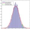 |
Fig. 1 Comparison of Gaussian PDF for estimator λ/σλ with its true estimated distribution. A 2σ significance using the Gaussian PDF corresponds in fact to a 2.5σ detection with the true distribution. (Calculation for 2MASS survey, see Sect. 6.) |
Another key problem is the estimation of the signal significance. We find that most approaches in the literature assume that the probability distribution function (PDF) of the estimator is Gaussian. In Fig. 1 we evaluate the estimator’s PDF (under the null hypothesis) for the ISW signal from the 2MASS survey (see Sect. 6) using a Monte-Carlo method (purple bars) and compare it with a Gaussian PDF (red solid line). The distributions’ tails differ, which leads to a bias in the confidence level for positive data (i.e., data with an ISW signal). For the 2MASS survey, a 2σ detection with a Gaussian assumption (vertical solid/green line) corresponds in fact to a 2.5σ detection using the true underlying PDF. In this case, the signal amplitude is underestimated with the Gaussian assumption. This behavior has also been studied for marginal detections by Bassett & Afshordi (2010). To avoid this bias, we recommend that the PDF be estimated and not assumed Gaussian.
Finally, there is not one “ideal” statistical method. Different methods have both advantages and disadvantages and a combination of different methods can prove complementary.
4.2. The Saclay method
 |
Fig. 2 Description of the steps involved in our method for detecting the ISW effect. Tests 1 to 3 are complementary and ask different statistical questions. |
We present here a new ISW detection method that uses the fields as input (and not the spectra). As we have seen, several statistical tests are interesting in the sense that they do not address the same questions. Therefore, we believe that a solid ISW detection method should test
-
1.
The correlation detection: this test is independent of thecosmology.
-
2.
The amplitude estimation: this will seek for a specific signal.
-
3.
The model comparison: this allows us to check whether the model with ISW is preferred to the model without ISW.
Using the fields instead of the spectra means we must deal with the problem of missing data, which we solve with a sparse inpainting technique (see Appendix A). This method has already been applied with success for CMB lensing estimations (Perotto et al. 2010).
The last important question is how we estimate the final detection level. As explained before, the z-score asymptotically follows a Gaussian distribution and so a bootstrap or Monte-Carlo method is required to derive the correct p-value from the true test distribution.
4.2.1. Methodology
Our optimal strategy (summarised by Fig. 2) for ISW detection is the following:
-
1.
Apply sparse inpainting to both the galaxy and CMB maps thatmay have different masks, essentially reconstructing missingdata around the Galactic plane and bulge.
-
2.
Test for simple correlation using a double bootstrap (one to estimate the variance and another to estimate the confidence) and using the fields as input. This returns a model-independent detection level.
-
3.
Reconstruct the ISW signal using expected cosmology and the inpainted galaxy density map.
-
4.
Estimate the signal amplitude using the fields as input, and apply a bootstrap (or MC) to the estimator. This validates both the signal and the model.
-
5.
Apply the model comparison test using the fields as input (see Sect. 4.2.2), essentially testing whether the data prefers a fiducial (e.g., ΛCDM) model over the null hypothesis, and measure relative fit of models.
Because we choose to work with the fields, the very first step is to deal with the missing data. This is an ill-posed problem, which can be solved using sparse inpainting (see Appendix A for more details). This approach reconstructs the entirety of the field, including along the Galactic plane and bulge. We show in Sect. 5 that the use of sparse inpainting does not introduce a bias in the detection of the ISW effect.
We then perform a correlation detection on the reconstructed fields data using a double bootstrap (see Appendix B.1). Experiments show that the bootstrap tends to over-estimate the confidence interval, especially when the p-values are low. This is why the obtained detection must be used as an indicator when near a significant value (for high p-values, the bootstrap remains accurate).
The second test evaluates the signal amplitude, which validates both the presence of a signal and the chosen model. Bootstrap methods can also be used here because they use no assumption on the underlying cosmology. However, since the accuracy of bootstrap depends on the quantity of observed elements, it may become inaccurate for low p-value, i.e., when, there is detection. In that case, Monte-Carlo (MC) will provide more accurate p-values and, for example, with 106 MC simulations, we have an accuracy of about 1/1000.
This second test compares the ISW signal with a fiducial model, but does not consider the possibility that the measured signal could in fact be consistent with the “null hypothesis”. So even with a significant signal, a third test is necessary. This more pertinent question is addressed by using the “Model Comparison” method (defined in Sect. 4.2.2), for the first time using the fields approach.
In conclusion, our method consists of a series of complementary tests, which together answer several questions. The first test seeks the presence of a correlation between two fields, without any referring cosmology. The second model-dependent test searches a given signal and tests its nullity. The third test asks whether the data prefer a fiducial ISW signal over the null hypothesis.
4.2.2. “Field” model comparison
We define here the model comparison technique using the fields approach, which has until now not been used in the literature. Using a generalised likelihood ratio approach, the quantity to measure is  (24)Theoretically, K6 convergences asymptotically to a χ2 variable with a certain number of d.o.f.’s. Because we only have one observation, we cannot assume (asymptotic) convergence. We can, however, use a Monte Carlo approach to estimate the p-value of the test under the H0 hypothesis.
The p-value is defined as the probability that under H0 the test value can be over a given K6, i.e.,  , where p is the probability distribution of the test under the H0 hypothesis. By simulating primordial CMB for a fiducial cosmology, these values can be easily computed. Then the p-value gives us a confidence on rejecting the H0 hypothesis.
Notice that the same procedure for the p-value estimation can be applied on K4 (Eq. (22)), even on K1 (Eq. (15)) and K3 (Eq. (17)) for the power spectra methods. We will refer to this p-value estimation as the Monte-Carlo estimation below, because we theoretically know the distribution under the null hypothesis; the primordial CMB is supposed to come from a Gaussian random process.
5. Validation of the Saclay method
In order to validate the Saclay method, we estimate the detection level expected using WMAP 7 data for the CMB and 2MASS and Euclid data for the galaxy data (see Sect. 6 for a description of WMAP and 2MASS data sets). We quantify the effect of the inpainting process on CMB maps with and without an ISW signal. We do this by simulating 2MASS-like and Euclid-like Gaussian and lognormal galaxy distributions and WMAP7-like Gaussian CMB maps (using cosmological parameters from Table 6) both with and without an ISW signal. We then apply our method to attempt a detection of the ISW signal. We do this both on full-sky maps and on masked data where we reconstruct data behind the mask using the sparse inpainting technique (the masks we use are as described in 6.1 and 6.2).
For each simulation, we run the three-step Saclay method. Except for the cross-correlation method, where we use 100 iterations for the 2MASS-like and 1000 for Euclid-like simulations for the p-value estimation and 201 for the variance estimation (nested bootstrap), every other Monte-Carlo process was performed using 10 000 iterations. All tests were performed inside the spherical harmonics domain with ℓ ∈ [2,100] for 2MASS and ℓ = [2,350] for a Euclid-like survey.
For the Euclid-like survey, we consider a galaxy distribution as defined in Amara & Réfrégier (2007), with mean redshift zm = 0.8 and slopes α = 2,β = 1.5. We reconstruct the ISW effect created by the projected galaxy distribution of the Euclid survey by considering only one large redshift bin. In the future, it could be possible to refine this reconstructed map by considering tomographic bins, or using information from the spectroscopic survey. Because sky-coverage maps are not yet available for Euclid, we consider the same mask as for 2MASS and inpaint regions with missing data following Sect. 6.3. We choose do to this rather than simply assume a value for the fraction of sky covered (fsky), to consider more realistic problems relating to the shape of the mask, and to test our inpainting method.
5.1. Expected level of detection
The expected detection levels (in units of σ) are reported in Table 3 (2MASS) and Table 4 (Euclid). Methods 1–3 correspond to the three-step method described in Fig. 2, where (b) and (MC) denote bootstrap and Monte Carlo evaluations of the variance and the p-value of the test. The p-values are converted as a σ value using the following formula:  (25)where p is the p-value, s the corresponding σ-score and erf-1 the inverse error function.
The 2MASS simulations (Table 3) show that we expect the same level of significance for an ISW detection, whether the mass tracer follows a Gaussian or a lognormal distribution. In either case the significance is low, around 1σ ± 1σ. This means that for 2MASS-like survey, we have a signal to noise ratio (S/N) around 1σ. We see no major difference between the expected detection levels of M2 and M3. The only difference is for M1 (but there is still agreement with M2 and M3 within 1σ error bars) – this may be because that the bootstrap technique is more efficient for Gaussian assumptions.
We also apply our method to CMB simulations with no ISW signal present (left two columns of Table 3), and find a lower detection significance than when an ISW signal is present. This is true even when inpainting is used to recover missing data, showing that the inpainting method does not introduce spurious correlations.
In any case, all methods suggest it is difficult to detect the ISW signal with high significance using the 2MASS data as a local tracer of the matter distribution.
In Table 4 we show that an Euclid-like survey, which is optimally designed for an ISW detection (see, Douspis et al. 2008), permits a much higher detection than with a 2MASS survey. As with 2MASS simulations, we notice that M2 and M3 return similar detection levels, which are lower than M1. Inclusion of masked data reduced the significance, but our inpainting method does not introduce spurious correlations because inpainted maps with no ISW do not return a detection. For a Euclid-like survey with incomplete sky coverage, we can expect to show that the data prefers an ISW component over no dark energy (M3) at the 5σ level, and detect a cross-correlation signal at the ~ 7σ level. We find no significant differences in the detection levels when the simulations are assumed lognormal or Gaussian.
Expected p-values for inpainted maps of ISW signal for a 2MASS-like local tracer of mass using Monte-Carlo or bootstrap methods for the first two steps of the Saclay method.
We also investigate the performance of the wild bootstrap method for the confidence estimation. Table 5 shows the p-values estimated using Monte-Carlo procedure and wild bootstrap for the first two methods of the three-step Saclay method. Notice that the bootstrap results are almost equivalent to Monte-Carlo ones. We found that the bootstrap method was not always reliable when the p-value became low because the precision of the bootstrap depends on both the number of bootstrap samples (as any MC-like process) and the number of observed elements. This last dependence makes the bootstrap uncertain when the detection is almost certain, that is why we consider the bootstrapped cross-correlation as an indicator that needs refinement when the results are very significant.
5.2. Power of the tests
In order to investigate the different strengths of each method, we also evaluated the rate of true positives vs. the number of false positives (i.e., false detections) – this information is summarised in Fig. 3 which shows receiver operating characteristic (ROC) curves. The construction of the ROC curve requires the computation of p-values for several simulated cases (i.e., simulations with and without an ISW signal), which are then sorted by value. For each p-value or threshold, the corresponding false positive and true positive rates are computed.
Generally, a more sensitive method may be more permissive and so will return a higher proportion of false detections. An ideal method will have a ROC curve above the diagonal from (0, 1) to (1, 1). Similarly, a poor detector will produce a curve below the diagonal, which corresponds to odds worse than tossing a coin. The X-axis corresponds to the false positive rate, i.e., the ratio of CMB maps without ISW where ISW signal is detected at the current threshold. The Y-axis corresponds to the true positive rate, i.e., the ratio of CMB maps with ISW where ISW signal is detected at the current threshold. We recall that a point on the ROC curve corresponds to a threshold.
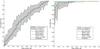 |
Fig. 3 ROC curves for the three-step Saclay method for the 2MASS survey (left) and the Euclid survey (right). Note the axes in the right-hand panel are different from the left-hand panel. The statistical methods correspond to fields model test (thin solid green, Method 3 in Table 3), field amplitude estimation (dot-dashed blue, Method 2), simple correlation (dashed red, Method 1). For the 2MASS survey, all methods are inside the 1σ error bar of the field’s amplitude estimation and so are nearly equivalent. For the Euclid-like survey, the statistics return much better values than for 2MASS (i.e., the ROC curves are far from the diagonal). The simple correlation method will return more false positives than the other two methods, which are nearly identical. The ROC curves of the simple correlation test differs sometimes by more than 1σ at some points from the other two methods and so is expected to perform differently. |
Figure 3 shows the ROC curves for three methods applied to a 2MASS-like survey (left) and a Euclid-like survey (right): fields model test (thin solid green), field amplitude estimation (dot-dashed blue), simple correlation (dashed red). For the 2MASS survey, all methods are inside the 1σ error bar of the field’s amplitude estimation and so are nearly equivalent, i.e., no method performs better than the others.
For the Euclid-like survey, the statistics return much better values than for 2MASS (i.e., the ROC curves are far from the diagonal). The simple correlation method will return more false positives than the other two methods, which are nearly identical. The ROC curves for each method differ by more than 1σ at some points and consequently different methods will perform differently.
6. The ISW signal in WMAP7 from 2MASS galaxies
We apply the new detection method described in Sect. 4 to WMAP7 data (Jarosik et al. 2011) and the 2MASS galaxy survey, which has been extensively used as a tracer of mass for the ISW signal (see Table 1). We describe first the data in Sects. 6.1 and 6.2. In Sect. 6.3 we describe the inpainting process that we apply to both CMB and galaxy data. In Sect. 6.4 we present the detection results.
6.1. WMAP
For the CMB data, we use several maps from NASA Wilkinson Microwave Anisotropy Probe: the internal linear combination map (ILC) for years 5 and 7 (WMAP5, Komatsu et al. 2009) (WMAP7, Jarosik et al. 2011) and the ILC map by Delabrouille et al. (2009), which was reconstructed using a needlets technique. We avoid regions that are contaminated by Galactic emission by applying the Kq85 temperature mask – which roughly corresponds to the Kp2 mask from the third year release (see Fig. 4). We also substract the kinetic Doppler quadrupole contribution from the data. WMAP simulations used to produce Tables 3 and 4 use WMAP 7 best-fit parameters for a flat ΛCDM universe (see Table 6).
Best-fit WMAP 7 cosmological parameters used throughout this paper.
6.2. 2MASS galaxy survey
The 2 Micron All-Sky Survey (2MASS) is a publicly available full-sky extended source catalogue (XSC) selected in the near-IR (Jarrett et al. 2000). The near-IR selection means galaxies are surveyed deep into the Galactic plane, meaning 2MASS has a very large sky coverage, ideal for detecting the ISW signal.
Following (Afshordi et al. 2004), we create a mask to exclude regions of sky where XSC is unreliable using the IR reddening maps of Schlegel et al. (1998). Using Ak = 0.367 × E(B − V), Afshordi et al. (2004) find a limit AK < 0.05 for which 2MASS is seen to 98% complete for K20 < 13.85, where K20 is the Ks-band isophotal magnitude. Masking areas with AK > 0.05 leaves 69% of the sky and approximately 828 000 galaxies for the analysis (see Fig. 4).
We use the redshift distribution computed by Afshordi et al. (2004) (and also used in Rassat et al. 2007), and to maximise the signal, we consider one overall bin for magnitudes 12 < K < 14. The redshift distribution for 2MASS is that shown in Fig. 1 of Rassat et al. (2007) (solid black line) and peaks at z ~ 0.073. The authors also showed that the small angle approximation could be used for calculations relating to 2MASS, so Eqs. (10) and (4) can be replaced by their simpler small-angle form: ![\begin{equation} C_{\rm gT}(\ell) = \frac{-3bH_0^2\Omega_{m,0}}{c^3(\ell+1/2)^2}\int \rm{d} {\it r \Theta D^2 H [f-1]P\left(\frac{\ell+1/2}{r}\right)}, \end{equation}](/articles/aa/full_html/2011/10/aa15893-10/aa15893-10-eq180.png) (26)and
(26)and  (27)We estimate the bias from the 2MASS galaxy power spectrum using the cosmology in Table 6 and find b = 1.27 ± 0.03, which is lower than that found in Rassat et al. (2007).
6.3. Applying sparse inpainting to CMB and galaxy data
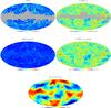 |
Fig. 4 Top: 2MASS map with mask (left) and WMAP 7 ILC map with mask (right). Middle: reconstructed 2MASS (left) and WMAP 7 ILC (right) maps using our inpainting method. Bottom: reconstructed ISW temperature field from the 2MASS galaxies calculated using Eq. (20). For better visualisation of the maps as an input of the Saclay method, we consider only the information inside ℓ ∈ [2,200]. |
As discussed in Sect. 4, regions of missing data in galaxy and CMB maps constitute an ill-posed problem when using a “field” based method. We propose to use sparse inpainting (see Starck et al. 2010, and Appendix A) to reconstruct the field in the regions of missing data.
We apply this method to both the WMAP7 and 2MASS maps and show the reconstructed maps in Fig. 4. All maps are pixelised using the HEALPix software (Górski et al. 2002; Gorski et al. 2005) with resolution corresponding to NSIDE = 512. The top two figures show 2MASS data (left) and ILC map (right) with the masks in grey. The two figures in the middle show the reconstructed density fields for 2MASS data (left) and the ILC map (right). The bottom two figures show the reconstruction of the ISW field using the inpainted 2MASS density map and Eq. (20) (for clarity, the first two multipoles (ℓ = 0,1) are not present in this map).
6.4. ISW detection using 2MASS and WMAP7 data
We use the Saclay method (Sect. 4) on WMAP7 and 2MASS data with 106 iterations for the Monte-Carlo iterations, 1000 iterations for both bootstrap and nested bootstrap of the correlation detection, and search for the ISW signal. In order to test the effect of including smaller (and possibly non-linear) scales, we perform the analysis for three different ℓ-ranges: ℓ ∈ [ℓmin,50], [ℓmin,100], [ℓmin,200], where ℓmin = 2 or 3. We notice that inclusion or exclusion of the quadrupole (ℓ = 2) can affect the significance level slighty, which is why we chose two values for ℓmin. We report our measured detection levels in Table 8. We recall the expected detections for 2MASS in Table 7, which can also be found in the more complete set of results presented in Table 3.
The results in Table 8 are compatible with the results in Table 3 within the errors bars. Rassat et al. (2007) used a spectra model-comparison method over ℓ = [3 − 30] and found that the model with dark energy was marginally preferred over the null hypothesis. Over a range ℓ = [2/3 − 50], using a fields model-comparison method, we find that a model with dark energy is preferred over the null hypothesis at the 0.9–1.2σ level, depending on the map. More generally, our results are compatible with the earliest ISW measurement using 2MASS data (Afshordi et al. 2004; Rassat et al. 2007) and lie in the 0.8–1.1σ range depending on the data and statistical test used.
The simple correlation test tends to report marginally higher detection levels than the field amplitude and model comparison tests, and the model comparison test similar values as the field amplitude test, which is compatible with the predictions from the ROC curves in Fig. 3.
7. Discussion
We have extensively reviewed the numerous methods in the literature that are used to detect and measure the presence of an ISW signal using maps for the CMB and local tracers of mass. We noticed that the variety of methods used can lead to different and conflicting conclusions. We also noted two broad classes of methods: one that uses the cross-correlation spectrum as the measure and the other that uses the reconstructed ISW temperature field.
We identified the advantages and disadvantages of all methods used in the literature and conclude that
-
1.
Using the fields (instead of spectra) as input required only theprimordial CMB to be Gaussian. This requires a reconstructionof the ISW field, which is difficult with missing data.
-
2.
The ill-posed problem of missing data can be solved using sparse inpainting, a method which does not introduce spurious correlations between maps.
-
3.
Assuming the estimator was Gaussian led to an under-estimation of the signal estimation.
-
4.
A series of statistical tests was able to provide complementary information.
This led us to construct a new and complete method for detecting and measuring the ISW effect. The method is summarised as follows:
-
1.
Apply sparse inpainting to both the galaxy and CMB maps,which may have different masks, essentially reconstructingmissing data around the Galactic plane and bulge.
-
2.
Test for simple correlation using a double bootstrap (one to estimate the variance and another to estimate the confidence) and the fields as input. This returns a model-independent detection level.
-
3.
Reconstruct the ISW signal using expected cosmology and the inpainted galaxy density map.
-
4.
Estimate the signal amplitude using the fields as input, and apply a bootstrap (or MC) to the estimator. This validates both the signal and the model.
-
5.
Apply the fields model comparison test, essentially testing whether the data prefers a given model over the null hypothesis, and measure relative fit of models.
The method we present makes only one assumption: that the primordial CMB temperature field behaves like a Gaussian random field. The method is general in that it “allows” the galaxy field to behave as a lognormal field, but does not automatically assume that the galaxy field is lognormal.
We first applied our method to 2MASS and Euclid simulations. We find that it is difficult to detect the ISW significantly using 2MASS simulations, and find no difference between assuming the underlying galaxy field to be Gaussian or lognormal, and only mild differences depending on the statistical test used. With a Euclid-like survey, we expect high detection levels, even with incomplete sky coverage – we expect ~7σ detection level using the simple correlation method, and ~5σ detection level using the fields amplitude or method comparison techniques. These detections levels are the same whether the Euclid galaxy field follows a Gaussian or lognormal distribution. Our results also show that the inpainting method does not introduce spurious correlations between maps.
We applied this method to WMAP7 and 2MASS data, and found that our results were comparable with early detections of the ISW signal using 2MASS data (Afshordi et al. 2004; Rassat et al. 2007) and lay roughly in the 1–1.2σ range. These results are also compatible with the simulations we ran for the 2MASS survey.
The last test we performed, the model comparison test, asks the much more pertinent question of whether the data prefers a ΛCDM model to the null hypothesis (i.e., no curvature and no dark energy). Using this test, we find a 0.8−1.2σ detection for ranges ℓ = [2/3−50] and 0.9 − 1.1σ for ranges ℓ = [2/3−100/200]. A by-product of this measurement is the reconstruction of the temperature ISW field from 2MASS galaxies, reconstructed with full sky coverage.
By applying our method to different estimations of CMB maps, we highlight the importance of component separation on the ISW detection. Table 8 shows scores between 1.0–1.2σ on different WMAP maps. We were also able to detect the ISW signal at 2.0σ using a another map (not presented in this paper). The influence of the component separation method on the quality of the estimation needs to be more deeply understood in future works.
Acknowledgments
This work has been supported by the European Research Council grant SparseAstro (ERC-228261). We thank Niayesh Afshordi, Ofer Lahav, John Peacock, Alexandre Réfrégier and the anonymous referee for useful discussions. We also thank Jacques Delabrouille for providing the needlets ILC 5yr map from the WMAP 5yr data. We used iCosmo1 software (Refregier et al. 2011), Healpix software (Górski et al. 2002; Gorski et al. 2005), ISAP2 software, the 2MASS catalogue3, the WMAP data4 and the Galaxy extinction maps of Schlegel et al. (1998).
References
- Abrial, P., Moudden, Y., Starck, J., et al. 2007, J. Fourier Anal. Appl., 13, 729 [Google Scholar]
- Abrial, P., Moudden, Y., Starck, J.-L., et al. 2008, Statist. Methodol., 5, 289 [Google Scholar]
- Adelman-McCarthy, J. K., Agüeros, M. A., Allam, S. S., et al. 2008, ApJS, 175, 297 [NASA ADS] [CrossRef] [Google Scholar]
- Afshordi, N., Loh, Y.-S., & Strauss, M. A. 2004, Phys. Rev. D, 69, 083524 [NASA ADS] [CrossRef] [Google Scholar]
- Afshordi, N., Slosar, A., & Wang, Y. 2011, J. Cosmol. Astropart. Phys., 1, 19 [NASA ADS] [CrossRef] [Google Scholar]
- Agüeros, M. A., Anderson, S. F., Margon, B., et al. 2006, AJ, 131, 1740 [NASA ADS] [CrossRef] [Google Scholar]
- Albrecht, A., Bernstein, G., Cahn, R., et al. 2006 [arXiv:0609591] [Google Scholar]
- Amara, A., & Réfrégier, A. 2007, MNRAS, 381, 1018 [NASA ADS] [CrossRef] [Google Scholar]
- Anderson, S. F., Fan, X., Richards, G. T., et al. 2001, AJ, 122, 503 [NASA ADS] [CrossRef] [Google Scholar]
- Bassett, B. A., & Afshordi, N. 2010 [arXiv:1005.1664] [Google Scholar]
- Bennett, C. L., Smoot, G. F., & Kogut, A. 1990, in BAAS, 22, 1336 [Google Scholar]
- Bernardeau, F., Colombi, S., Gaztañaga, E., & Scoccimarro, R. 2002, Phys. Rep., 367, 1 [NASA ADS] [CrossRef] [EDP Sciences] [MathSciNet] [Google Scholar]
- Boldt, E. 1987, Phys. Rep., 146, 215 [NASA ADS] [CrossRef] [Google Scholar]
- Boughn, S., & Crittenden, R. 2004, Nature, 427, 45 [NASA ADS] [CrossRef] [EDP Sciences] [PubMed] [Google Scholar]
- Boughn, S. P., & Crittenden, R. G. 2002, Phys. Rev. Lett., 88, 021302 [NASA ADS] [CrossRef] [Google Scholar]
- Boughn, S. P., & Crittenden, R. G. 2005, New Astron. Rev., 49, 75 [NASA ADS] [CrossRef] [Google Scholar]
- Boughn, S. P., Crittenden, R. G., & Turok, N. G. 1998, New A, 3, 275 [NASA ADS] [CrossRef] [Google Scholar]
- Cabré, A., Gaztañaga, E., Manera, M., Fosalba, P., & Castander, F. 2006, MNRAS, 372, L23 [NASA ADS] [Google Scholar]
- Cabré, A., Fosalba, P., Gaztañaga, E., & Manera, M. 2007, MNRAS, 381, 1347 [NASA ADS] [CrossRef] [Google Scholar]
- Cai, Y., Cole, S., Jenkins, A., & Frenk, C. S. 2010, MNRAS, 407, 201 [NASA ADS] [CrossRef] [Google Scholar]
- Carroll, S. M., de Felice, A., Duvvuri, V., et al. 2005, Phys. Rev. D, 71, 063513 [NASA ADS] [CrossRef] [Google Scholar]
- Cole, S., Norberg, P., Baugh, C. M., et al. 2001, MNRAS, 326, 255 [NASA ADS] [CrossRef] [Google Scholar]
- Combettes, P. L., & Wajs, V. R. 2005, SIAM Multi. Model. Simul., 4, 1168 [Google Scholar]
- Condon, J. J., Cotton, W. D., Greisen, E. W., et al. 1998, AJ, 115, 1693 [NASA ADS] [CrossRef] [Google Scholar]
- Corasaniti, P., Giannantonio, T., & Melchiorri, A. 2005, Phys. Rev. D, 71, 123521 [NASA ADS] [CrossRef] [Google Scholar]
- Crittenden, R. G., & Turok, N. 1996, Phys. Rev. Lett., 76, 575 [NASA ADS] [CrossRef] [Google Scholar]
- Davidson, A., & MacKinnon, J. G. 2006, J. Econom., 133, 421 [CrossRef] [Google Scholar]
- Davidson, R., & Flachaire, E. 2008, J. Econometrics, 146, 162 [CrossRef] [Google Scholar]
- Delabrouille, J., Cardoso, J., Le Jeune, M., et al. 2009, A&A, 493, 835 [NASA ADS] [CrossRef] [EDP Sciences] [Google Scholar]
- DiCiccio, T. J., & Efron, B. 1996, Stat. Sci., 11, 189 [CrossRef] [Google Scholar]
- Dodelson, S. 2003, Modern cosmology (Modern cosmology/Scott Dodelson (Amsterdam, Netherlands: Academic Press= ISBN 0-12-219141-2, 2003, XIII + 440) [Google Scholar]
- Donoho, D., & Huo, X. 2001, IEEE Trans. Info. Theo., 47, 2845 [Google Scholar]
- Doroshkevich, A., Tucker, D. L., Allam, S., & Way, M. J. 2004, A&A, 418, 7 [NASA ADS] [CrossRef] [EDP Sciences] [Google Scholar]
- Douspis, M., Castro, P. G., Caprini, C., & Aghanim, N. 2008, AAP, 485, 395 [Google Scholar]
- Efron, B. 1979, Ann. Statistics, 7, 1 [Google Scholar]
- Efron, B. 1987, The Jackknife, the Bootstrap, and Other Resampling Plans, CBMS-NSF Regional Conference Series in Applied Mathematics (Society for Industrial Mathematics) [Google Scholar]
- Efstathiou, G. 2004, MNRAS, 349, 603 [NASA ADS] [CrossRef] [Google Scholar]
- Elad, M., Starck, J.-L., Querre, P., & Donoho, D. 2005, Appl. Comput. Harm. Anal., 19, 340 [Google Scholar]
- Fadili, M. J., Starck, J.-L., & Murtagh, F. 2009, Comp. J., 52, 64 [CrossRef] [Google Scholar]
- Flachaire, E. 2005, Computational Statistics & Data Analysis, 49, 361, 2nd CSDA Special Issue on Computational Econometrics [CrossRef] [Google Scholar]
- Fosalba, P., & Gaztañaga, E. 2004, MNRAS, 350, L37 [NASA ADS] [CrossRef] [Google Scholar]
- Fosalba, P., Gaztañaga, E., & Castander, F. 2003, ApJ, 597, L89 [NASA ADS] [CrossRef] [Google Scholar]
- Francis, C. L., & Peacock, J. A. 2010a, MNRAS, 406, 14 [Google Scholar]
- Francis, C. L., & Peacock, J. A. 2010b, MNRAS, 406, 2 [NASA ADS] [CrossRef] [Google Scholar]
- Frommert, M., Enßlin, T. A., & Kitaura, F. S. 2008, MNRAS, 391, 1315 [NASA ADS] [CrossRef] [Google Scholar]
- Gaztañaga, E., Manera, M., & Multamaki, T. 2006, MNRAS, 365, 171 [NASA ADS] [CrossRef] [Google Scholar]
- Giannantonio, T., Crittenden, R. G., Nichol, R. C., et al. 2006, Phys. Rev. D, 74, 063520 [NASA ADS] [CrossRef] [Google Scholar]
- Giannantonio, T., Scranton, R., Crittenden, R. G., et al. 2008, Phys. Rev. D, 77, 123520 [NASA ADS] [CrossRef] [Google Scholar]
- Górski, K. M., Banday, A. J., Hivon, E., & Wandelt, B. D. 2002, in Astronomical Data Analysis Software and Systems XI, ed. D. A. Bohlender, D. Durand, & T. H. Handley, ASP Conf. Ser., 281 [Google Scholar]
- Gorski, K. M., Hivon, E., Banday, A. J., et al. 2005, ApJ, 622, 759 [NASA ADS] [CrossRef] [Google Scholar]
- Granett, B. R., Neyrinck, M. C., & Szapudi, I. 2009, ApJ, 701, 414 [NASA ADS] [CrossRef] [Google Scholar]
- Hadamard, J. 1902, Sur les problèmes aux dérivées partielles et leur signification physique [Google Scholar]
- Hall, P. 1995, The Bootstrap and Edgeworth Expansion, Springer Series in Statistics (Springer) [Google Scholar]
- Hamimeche, S., & Lewis, A. 2008, Phys. Rev. D, 77, 103013 [NASA ADS] [CrossRef] [Google Scholar]
- Hernández-Monteagudo, C. 2008, A&A, 490, 15 [NASA ADS] [CrossRef] [EDP Sciences] [Google Scholar]
- Hernández-Monteagudo, C. 2010, A&A, 520, A101 [NASA ADS] [CrossRef] [EDP Sciences] [Google Scholar]
- Hivon, E., Górski, K. M., Netterfield, C. B., et al. 2002, ApJ, 567, 2 [NASA ADS] [CrossRef] [Google Scholar]
- Ho, S., Hirata, C., Padmanabhan, N., Seljak, U., & Bahcall, N. 2008, Phys. Rev. D, 78, 043519 [NASA ADS] [CrossRef] [Google Scholar]
- Jarosik, N., Bennett, C. L., Dunkley, J., et al. 2011, ApJS, 192, 14 [NASA ADS] [CrossRef] [Google Scholar]
- Jarrett, T. H., Chester, T., Cutri, R., et al. 2000, Astron. J., 119, 2498 [NASA ADS] [CrossRef] [Google Scholar]
- Kamionkowski, M., & Spergel, D. N. 1994, ApJ, 432, 7 [NASA ADS] [CrossRef] [Google Scholar]
- Kayo, I., Taruya, A., & Suto, Y. 2001, ApJ, 561, 22 [NASA ADS] [CrossRef] [Google Scholar]
- Kinkhabwala, A., & Kamionkowski, M. 1999, Phys. Rev. Lett., 82, 4172 [NASA ADS] [CrossRef] [Google Scholar]
- Komatsu, E., Dunkley, J., Nolta, M. R., et al. 2009, ApJS, 180, 330 [NASA ADS] [CrossRef] [Google Scholar]
- Liu, R. Y. 1988, Ann. Stat., 16, 1696 [Google Scholar]
- López-Corredoira, M., Sylos Labini, F., & Betancort-Rijo, J. 2010, A&A, 513, A3 [NASA ADS] [CrossRef] [EDP Sciences] [Google Scholar]
- Maddox, S. J., Efstathiou, G., Sutherland, W. J., & Loveday, J. 1990, MNRAS, 242, 43P [NASA ADS] [CrossRef] [Google Scholar]
- Mammen, E. 1993, Ann. Stat., 21, 255 [CrossRef] [Google Scholar]
- McEwen, J. D., Vielva, P., Hobson, M. P., Martínez-González, E., & Lasenby, A. N. 2007, MNRAS, 376, 1211 [NASA ADS] [CrossRef] [Google Scholar]
- McEwen, J. D., Wiaux, Y., Hobson, M. P., Vandergheynst, P., & Lasenby, A. N. 2008, MNRAS, 384, 1289 [NASA ADS] [CrossRef] [Google Scholar]
- Munshi, D., Valageas, P., Cooray, A., & Heavens, A. 2011, MNRAS, 414, 3173 [NASA ADS] [CrossRef] [Google Scholar]
- Nolta, M. R., Wright, E. L., Page, L., et al. 2004, ApJ, 608, 10 [NASA ADS] [CrossRef] [Google Scholar]
- Padmanabhan, N., et al. 2005, Phys. Rev. D, 72, 043525 [NASA ADS] [CrossRef] [Google Scholar]
- Peacock, J. A., Schneider, P., Efstathiou, G., et al. 2006, ESA-ESO Working Group on “Fundamental Cosmology”, Tech. Rep. [Google Scholar]
- Percival, W. J., Nichol, R. C., Eisenstein, D. J., et al. 2007a, ApJ, 657, 51 [NASA ADS] [CrossRef] [Google Scholar]
- Perotto, L., Bobin, J., Plaszczynski, S., Starck, J., & Lavabre, A. 2010, A&A, 519, A4 [NASA ADS] [CrossRef] [EDP Sciences] [Google Scholar]
- Pietrobon, D., Balbi, A., & Marinucci, D. 2006, Phys. Rev. D, 74, 043524 [NASA ADS] [CrossRef] [Google Scholar]
- Pires, S., Starck, J., Amara, A., et al. 2009, MNRAS, 395, 1265 [NASA ADS] [CrossRef] [Google Scholar]
- Pires, S., Starck, J., & Refregier, A. 2010, IEEE Signal Processing Magazine, 27, 76 [Google Scholar]
- Raccanelli, A., Bonaldi, A., Negrello, M., et al. 2008, MNRAS, 386, 2161 [NASA ADS] [CrossRef] [Google Scholar]
- Racine, J. S., & MacKinnon, J. G. 2007, Comput. Stat. Data Anal., 51, 5949 [CrossRef] [Google Scholar]
- Rassat, A., Land, K., Lahav, O., & Abdalla, F. B. 2007, MNRAS, 377, 1085 [NASA ADS] [CrossRef] [Google Scholar]
- Rauhut, H., & Ward, R. 2010 [arXiv:1003.0251] [Google Scholar]
- Refregier, A., Amara, A., Kitching, T. D., et al. 2010 [arXiv:1001.0061] [Google Scholar]
- Refregier, A., Amara, A., Kitching, T. D., & Rassat, A. 2011, A&A, 528, A33 [NASA ADS] [CrossRef] [EDP Sciences] [Google Scholar]
- Sachs, R. K., & Wolfe, A. M. 1967, ApJ, 147, 73 [NASA ADS] [CrossRef] [Google Scholar]
- Sawangwit, U., Shanks, T., Cannon, R. D., et al. 2010, MNRAS, 402, 2228 [NASA ADS] [CrossRef] [Google Scholar]
- Schaefer, B. M., Fotios Kalovidouris, A., & Heisenberg, L. 2011, MNRAS, 416, 1302 [NASA ADS] [CrossRef] [Google Scholar]
- Schlegel, D. J., Finkbeiner, D. P., & Davis, M. 1998, ApJ, 500, 525 [NASA ADS] [CrossRef] [Google Scholar]
- Schrabback, T., Hartlap, J., Joachimi, B., et al. 2010, A&A, 516, A63 [NASA ADS] [CrossRef] [EDP Sciences] [Google Scholar]
- Scranton, R., Connolly, A. J., Nichol, R. C., et al. 2003, unpublished [arXiv:0307335] [Google Scholar]
- Song, Y.-S., Hu, W., & Sawicki, I. 2007, prd, 75, 044004 [Google Scholar]
- Spergel, D. N., Verde, L., Peiris, H. V., et al. 2003, ApJS, 148, 175 [NASA ADS] [CrossRef] [Google Scholar]
- Starck, J.-L., Murtagh, F., & Fadili, M. 2010, Sparse Image and Signal Processing (Cambridge University Press) [Google Scholar]
- Vielva, P., Martínez-González, E., & Tucci, M. 2006, MNRAS, 365, 891 [NASA ADS] [CrossRef] [Google Scholar]
- Wild, V., Peacock, J. A., Lahav, O., et al. 2005, MNRAS, 356, 247 [NASA ADS] [CrossRef] [Google Scholar]
- Xia, J., Viel, M., Baccigalupi, C., & Matarrese, S. 2009, J. Cosmology Astropart. Phys., 9, 3 [Google Scholar]
Appendix A: Sparse inpainting
The goal of inpainting is to restore missing or damaged regions of an image in a way that the restored map has the same statistical properties as the underlying unmasked map (Elad et al. 2005). Sparse inpainting has been proposed for filling the gaps in CMB maps (Abrial et al. 2007, 2008) and for weak-lensing mass map reconstruction (Pires et al. 2009, 2010). In Perotto et al. (2010), it has been shown that the sparse inpainting method does not destroy the CMB weak-lensing signal, and is therefore an elegant way to handle the mask problem.
The inpainting problem can be defined as follows. Let X be the ideal complete image, Y the observed incomplete image (images can be fields on the sphere) and L the binary mask (i.e., L [k,l] = 1 if we have information at pixel (k,l), L [k,l] = 0 otherwise). In short, we have Y = LX.
Inpainting consists in recovering X knowing Y and L. The masking effect can be thought of as a loss of sparsity in the spherical harmonic domain because the information required to define the map has been spread across the spherical harmonic basis.
Sparsity means that most of the information is concentrated in a few coefficients, which when sorted from the largest to the smallest, follow an exponential decay. More details can be found in (Starck et al. 2010). In this paper, the chosen “dictionary” is the spherical harmonic domain.
Denoting the spherical harmonic basis as Φ (so ΦT is the spherical harmonic transform, i.e., the projector onto the spherical harmonic space), ||z||0 the l0 pseudo-norm, i.e., the number of non-zero entries in z and ||z|| the classical l2 norm (i.e., ||z||2 = ∑ k(zk)2), we thus want to minimise  (A.1)where σ stands for the noise standard deviation in the noisy case. It has also been shown that if X is sparse enough, the l0 pseudo-norm can also be replaced by the convex l1 norm (i.e., ||z||1 = ∑ k|zk|) (Donoho & Huo 2001). The solution of such an optimisation task can be obtained through an iterative thresholding algorithm called MCA (Elad et al. 2005; Fadili et al. 2009; Starck et al. 2010) :
  (A.2)where the nonlinear operator ΔΦ,λ(Z) consists of
-
1.
decomposing the signal Z on the dictionary Φ to derive the coefficients α = ΦTZ (i.e., α is the vector containing the aℓm coefficients).
-
2.
threshold the coefficients:
 , where the thresholding operator ρ can either be a hard thresholding (i.e., ρ(αi,λ) = αi if |αi| > λ and 0 otherwise) or a soft thresholding (i.e., ρ(αi,λ) = sign(αi)max(0,|αi| − λ)). The hard thresholding corresponds to the l0 optimisation problem, while the soft-threshold solves that for l1.
 -
3.
reconstruct
 from the thresholds coefficients
  .
.
The threshold parameter λn decreases with the iteration number and plays a role similar to the cooling parameter of the simulated annealing techniques, i.e., it allows the solution to escape from local minima.
It has been shown in Abrial et al. (2008) that this inpainting technique leads to accurate CMB recovery results. More details relative to this optimisation problem can be found in Combettes & Wajs (2005); Starck et al. (2010) and theoretical justifications for CMB sparse inpainting in Rauhut & Ward (2010). The software is available in the Multi-Resolution on the Sphere (MRS) package5.
Appendix B: Bootstrapping detection tests
Most detection methods rely on a z-score whose confidence is computed assuming a Gaussian distribution (see Sect. 3.2). This assumption is valid within the central limit theorem and so is not always true. Using an estimator of the true distribution will give more reliable confidence levels. To estimate the true distribution, two approaches are generally used: Monte-Carlo simulations when a model and its parameters are available or non-parametric bootstraps methods.
In order to build a fully non-parametric and cosmology independent correlation detection test, we propose to use the wild bootstrap to estimate both estimator variance and confidence interval. The remaining question will be the reliability of this test when bootstraps are sometimes known to underestimate confidence intervals. The answer to the question mainly depends on the choice of domain (e.g., pixels, spherical harmonics) and the method chosen for estimating.
Working with correlated data is difficult and estimated values are generally different to the true ones. We chose to work in the spherical harmonic domain, which produces heteroskedastic (i.e., the power spectrum is scale dependent) and uncorrelated data. For heteroskedastic and uncorrelated data, bootstraps methods such as wild bootstrap can be used. Flachaire (2005); Davidson & Flachaire (2008) showed the good behaviour of wild bootstrap in many situations. We propose here a short introduction to this method, which we use to estimate p-values and estimator variances.
B.1. Wild bootstrap and regression model
Bootstrap methods were introduced by Efron (1979) as a generalisation of the jackknife and its concept has been extended to many situations. For the regression case with heteroskedastic data, wild bootstrap was developed by Liu (1988), who established the ability of wild bootstrap to provide refinements for the linear regression model with heteroskedastic disturbances. Mammen (1993) showed that the wild bootstrap was asymptotically justified, in the sense that the asymptotic distribution of various statistics is the same as the asymptotic distribution of their wild bootstrap counterparts.
If you look at the correlation estimator (Eq. (11)) and the amplitude estimation (Eq. (21)), they both suppose an underlying linear model:  (B.1)where δO is the observed field which contains the signal of interest (e.g., CMB), δC a tracer of the signal of interest (e.g., matter density, ISW reconstruction), ρ is either the correlation coefficient and the amplitude of the signal (depending of the estimator) and σ is the noise that depends on the position.
The originality of the wild bootstrap is that its data generating process (DGP) creates new samples without any prior on the distribution of the noise. This process uses the residual, i.e.,  , where
  is the parameter estimate. Then, new samples are created using the formula
  where
where  indicates the bootstrapped version of the sample and ε is a random variable following a given distribution. The performance of the wild bootstrap mainly depends on the distribution of ε, which must fulfill some conditions like having a null mean and a unit variance.
Liu (1988) for example proposed to use Rademacher variables for the distribution, 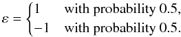 (B.4)Davidson & Flachaire (2008) showed that exact inference (up to a theoretical accuracy) is possible if
  is independent of all disturbance uℓm and if the test distribution is symmetric about 0. Moreover, the rate of convergence of the error in the rejection probabilities (ERP) is at most n − 3/2 with symmetric errors and n − 1/2 with asymmetric errors (n is the size of the observed sample). The ERP is the difference between the actual rejection frequency under the null hypothesis and the level of the test (e.g., about 0.045 for a 2σ detection). In other words, this is the precision error on the inferred p-value. Notice that it mainly depends on the sample size.
B.2. Parametric bootstrap
The wild bootstrap is very useful when little is known about the noise. However, sometimes the noise distribution is well known and its parameters can be estimated from the observations. In this case, it is possible to use this distribution to generate new samples. For example, if we model the CMB primordial distribution by a multivariate normal law, the  can be generated as,
  where CCMB is the power spectrum of the primordial CMB. Notice that using the theoretical CMB power spectra leads to a Monte-Carlo method, which is then dependent on the chosen cosmology.
B.3. Estimating the estimator variance
When the variance of an estimator is unknown, a bootstrap can be used to estimate it with the following scheme:
-
1.
Estimate the parameter vector
from the observed data; -
2.
create B bootstrap samples using Eq. (B.2) or another method (see Sect. B.2);
-
3.
estimate the parameter vector
 , i ∈ [1,B] for each bootstrap sample;
 -
4.
compute the estimation of the variance of the estimator,
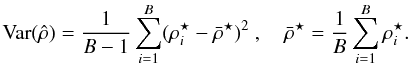 (B.5)
(B.5)
B.4. Estimating the p-value of a test
The estimation of the confidence interval of a hypothesis test requires the generation of samples under the null hypothesis. Inside the wild bootstrap DGP that leads to set  when using Eq. (B.2) for new samples (it also remains true with a parametric bootstrap). Using this property, the scheme for computing the p-value is to
-
1.
Estimate the parameter vector and its variance (e.g., using theprevious scheme in B.3),
and  ;
; - 2.
-
3.
create B bootstrap samples which follow the null hypothesis using B.2 (or Sect. B.2) and
; -
4.
estimate the parameter
and its variance  for each bootstrap sample i ∈ [1,B];
 -
5.
compute the correspondant z-score,
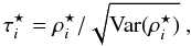 (B.7)for each bootstrap sample i ∈ [1,B];
 -
6.
compute the bootstrapped p-value,
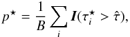 (B.8)where I denotes the indicator function, which is equal to 1 when its argument is true, and 0 otherwise.
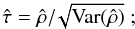
Equation (B.8) can be a little too sharp and may lead to inaccurate results when the answer is just between two bootstrap samples. One way to reduce this effect is by smoothing the empirical distribution (Racine & MacKinnon 2007), for example with a Gaussian kernel, 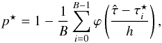 (B.9)where ϕ is the Gaussian cumulative distribution function and h the bandwidth of the kernel (chosen depending on the required precision, see Racine & MacKinnon 2007).
B.5. Reliability of bootstrap
One can be perplexed by the efficiency and the reliability of the bootstrap method. Many studies have proved that these methods outperform asymptotic tests (i.e., using the asymptotic distribution, see Davidson & MacKinnon 2006) and sometimes perform almost as well as exact tests (i.e., with the true distribution, we refer the reader to Efron 1987; DiCiccio & Efron 1996; Hall 1995, for more information). The efficiency mostly depends on three key elements: 1) the data generating process (DGP) under both hypotheses (often generating under the alternative hypothesis is non trivial); 2) the number of observations; and 3) the number of bootstrapped samples. The variance on p is given by p(1 − p)/B, where B is the number of bootstraps. While the number of bootstrapped samples can be easily tackled, the DGP on the chosen method and the number of observations depends on many parameters (e.g., configuration, instruments, acquisition time). Even with the most efficient DGP, the precision of the bootstrap methods is limited by the number of observations, often in  , sometimes
  . In other words, bootstrap methods are mostly inaccurate when the observed value is at the tail of the involved distribution (and so a rare event). For example, a p-value estimated using 100 observations will be ± 0.1 and be inefficient for characterising high confidence, but can still be useful for rejecting.
All Tables
Meta-analysis of ISW detections to date and their reported statistical significance.
Review of advantages and disadvantages of measuring spectra vs. fields to infer an ISW detection (top). Review of statistical methods in the literature and their respective advantages and disadvantages (bottom).
Expected p-values for inpainted maps of ISW signal for a 2MASS-like local tracer of mass using Monte-Carlo or bootstrap methods for the first two steps of the Saclay method.
All Figures
|
Fig. 1 Comparison of Gaussian PDF for estimator λ/σλ with its true estimated distribution. A 2σ significance using the Gaussian PDF corresponds in fact to a 2.5σ detection with the true distribution. (Calculation for 2MASS survey, see Sect. 6.) |
| In the text | |
|
Fig. 2 Description of the steps involved in our method for detecting the ISW effect. Tests 1 to 3 are complementary and ask different statistical questions. |
| In the text | |
|
Fig. 3 ROC curves for the three-step Saclay method for the 2MASS survey (left) and the Euclid survey (right). Note the axes in the right-hand panel are different from the left-hand panel. The statistical methods correspond to fields model test (thin solid green, Method 3 in Table 3), field amplitude estimation (dot-dashed blue, Method 2), simple correlation (dashed red, Method 1). For the 2MASS survey, all methods are inside the 1σ error bar of the field’s amplitude estimation and so are nearly equivalent. For the Euclid-like survey, the statistics return much better values than for 2MASS (i.e., the ROC curves are far from the diagonal). The simple correlation method will return more false positives than the other two methods, which are nearly identical. The ROC curves of the simple correlation test differs sometimes by more than 1σ at some points from the other two methods and so is expected to perform differently. |
| In the text | |
|
Fig. 4 Top: 2MASS map with mask (left) and WMAP 7 ILC map with mask (right). Middle: reconstructed 2MASS (left) and WMAP 7 ILC (right) maps using our inpainting method. Bottom: reconstructed ISW temperature field from the 2MASS galaxies calculated using Eq. (20). For better visualisation of the maps as an input of the Saclay method, we consider only the information inside ℓ ∈ [2,200]. |
| In the text | |
Current usage metrics show cumulative count of Article Views (full-text article views including HTML views, PDF and ePub downloads, according to the available data) and Abstracts Views on Vision4Press platform.
Data correspond to usage on the plateform after 2015. The current usage metrics is available 48-96 hours after online publication and is updated daily on week days.
Initial download of the metrics may take a while.