| Issue |
A&A
Volume 534, October 2011
|
|
|---|---|---|
| Article Number | A35 | |
| Number of page(s) | 14 | |
| Section | Extragalactic astronomy | |
| DOI | https://doi.org/10.1051/0004-6361/201015670 | |
| Published online | 28 September 2011 | |
Distances and stellar population properties for 12 elliptical galaxies
1
INAF-Osservatorio Astronomico di Teramo, via M. Maggini snc, 64100 Teramo, Italy
e-mail: This email address is being protected from spambots. You need JavaScript enabled to view it.
2
Dipartimento di Scienze Fisiche, Università di Napoli Federico II, Compl. Univ. Monte S. Angelo, Ed. N, via Cinthia, 80126 Napoli, Italy
3 MECENAS, Università di Napoli Federico II and Università di Bari, Italy
Received: 1 September 2010
Accepted: 18 August 2011
Abstract
Aims. We use the surface brightness fluctuation (SBF) technique to derive the distances and analyse the radial behaviour of stellar populations in a sample of 12 elliptical galaxies. The data are I-band images collected with the FORS1 camera at the Very Large Telescope (VLT), drawn from the ESO archive. The main purpose of our analysis is to carry out the study of SBF magnitudes without relying on additional colour information that is normally required in SBF studies.
Methods. We measure I-band SBF magnitudes and SBF variations with galaxy radii, which is useful for stellar population studies. Unlike typical applications of the SBF technique, the absolute SBF magnitudes needed to evaluate the distance moduli are derived using the fluctuation star count,  .
.
Results. The distances obtained using the calibration taken from the literature show a good agreement with available estimates. We find a median ~0.2 mag difference between our and literature distance moduli, with the only exception of NGC 5090, which shows the I-band SBF ~ 1 mag brighter than expected. The median statistical and systematic errors are ~0.2 and ~0.1 mag, respectively. On these grounds we consider the test of deriving SBF distances based on the calibration to be successful. Taking into account that some of the previously estimated distances were made as long as 15 years ago, the new measurements provide an updated sketch on distances for a set of galaxies towards the region of the Great Attractor. Furthermore, gauging the SBF of the unresolved stellar systems has returned negative SBF radial gradients in the inner regions of five galaxies: a feature already known and explained by lower metallicity at larger galactic radii. Somehow unexpectedly, though, we detect positive SBF gradients at large radii ( ≳ 20 kpc) in nine targets. This behaviour, if it is not caused by some unaccounted observational bias, could be explained at least partly as a statistical effect on the stellar counts at these radii. Additional (near-IR) observations are necessary to confirm the real existence of this feature and to allow us to reach more robust conclusions.
Key words: galaxies: distances and redshifts / galaxies: photometry / galaxies: elliptical and lenticular, cD / galaxies: general / stars: statistics
© ESO, 2011
1. Introduction
A growing amount of public-domain data exists in the archives of most telescopes. No matter what the specific interests of the observers were, there are cases in which their observations are well-suited for other studies. The present paper makes use of public-domain data. In particular, we use archival I-band observations of 12 elliptical galaxies collected with the FORS1 (FOcal Reducer and low-dispersion Spectrograph) camera at the VLT to derive distances and to study stellar population properties of the targets with the surface brightness fluctuation technique (SBF hereafter; Tonry & Schneider 1988; Tonry et al. 1990).
The SBF magnitudes are a direct consequence of the discrete nature of the emitting sources in galaxies, i.e. stars (see, e.g., Tonry 1991; Lorenz et al. 1993; Ajhar & Tonry 1994; Jensen et al. 1996). In short, the SBF signal is generated by the Poissonian fluctuation of the surface brightness in the galaxy, which is caused by the statistical variation of the stellar counts in adjacent resolution elements. The SBF measure has proved to be a powerful distance indicator and an accurate tracer of stellar population properties because, to first order, optical and near-IR SBF magnitudes correspond to the mean luminosity of giant-branch stars (Tonry et al. 1990).
To derive distances, the amplitude of SBF magnitudes – measured by the ratio between the variance of the flux and the local mean flux (Tonry & Schneider 1988) – is typically calibrated by using the integrated colours of the galaxy. One of the earliest and most thoroughly analysed SBF calibrations is the I-band one, provided by Tonry et al. (2001) from the analysis of the SBF and V − I properties of ~300 galaxies in different environments and with different morphologies: ![Mathematical equation: \hbox{$\bar{M}_I=-1.74+4.5\cdot[(V{-}I)-1.15]$}](/articles/aa/full_html/2011/10/aa15670-10/aa15670-10-eq6.png) . The coupling of the calibrated SBF magnitude,
. The coupling of the calibrated SBF magnitude,  , with the measured
  , gives the distance modulus of the object in the usual way:
  .
.
Furthermore, a better understanding of the link between the SBF signal and the stellar population properties (e.g., age and chemical composition), has proved that multi-band SBF data can be used to efficiently constrain the physical characteristics of the stellar system host in a galaxy, mainly because some SBF colours are much less susceptible the age-metallicity degeneracy that affects other spectro-photometric indicators (O’Connell 1986; Worthey 1994). In this sense, the numerical modelling of the stellar populations plays a key role in revealing how SBF magnitudes and SBF colours are affected by stellar population changes (Buzzoni 1993; Worthey 1993; Blakeslee et al. 2001b; Cantiello et al. 2003; Raimondo et al. 2005).
In addition to the mean SBF magnitudes, radial variations in the SBF magnitude have been measured for several galaxies out to ~30 Mpc, providing an insight into the radial variations of stellar population properties (Pahre & Mould 1994; Sodemann & Thomsen 1995; Cantiello et al. 2005, 2007a). These SBF gradients represent a powerful and independent tool to understand how stellar populations have evolved within galaxies. As discusses by Cantiello et al. (2005), the radial change of SBF magnitudes, or SBF colours, in a galaxy can be a valuable tool to constrain formation mechanism theories: steep gradients – correlated with the galactic mass – support dissipative collapse scenarios (Carlberg 1984; Davies et al. 1993; Spolaor et al. 2009), while shallow gradients are expected in the hierarchical merging picture (Kauffmann et al. 1993; Bekki & Shioya 2001; La Barbera et al. 2004). Therefore, the radial behaviour of stellar population properties contains a footprint of the galaxy star-formation history but, while modern versions of the monolithic or hierarchical formation scenarios have shown that they are able to reproduce in part the observed behaviour of early-type galaxies, none of the proposed scenarios has proved to be decisively successful over the other (Kampakoglou et al. 2008; Foster et al. 2009). The SBF gradients measurements, which are independent of other spectro-photometric indicators, represent a new way for unveiling radial changes in the stellar population properties, providing useful complementary information on the age and metallicity gradients within galaxies.
As anticipated, the dataset used in this work consists of only I-band images. This did not allow us i) to use the typical standardisation of SBF magnitudes required for distance analysis – based on the relation between the and the integrated colour of the source – and ii) to study stellar populations with a multi-colour analysis. Nonetheless, we will show in the following sections that reliable distances can be derived using a different, less common, empirical calibration of based on the fluctuation star counts (Tonry et al. 2001). We will also make use of SBF radial profiles in galaxies to extract some information on the host stellar populations.
Before we proceed further, we emphasise that we intentionally intend to carry out our analysis based on the sole single-band data available from the VLT program described below. A number of SBF analyses are based on single-band images, like Sodemann & Thomsen (1995) or Fritz (2002). However, even when only I-band images were used, the authors used some colour information of the targets taken, e.g., from the literature. In contrast, we will conduct the SBF analysis without any colour calibration for the galaxies, consequently the distances and stellar populations with rely solely on the I-band data taken from the respective observing program.
Our choice is driven by various considerations. First and foremost, we aim to show that a self-consistent and accurate analysis of galaxy properties based on SBF magnitudes is feasible without observations in any other bands except the one used for the SBF measure itself. Second, for the sake of homogeneity, we decided in the calibration of SBF magnitudes to avoid any mixing of the present dataset with other data from the literature.
The paper is organised as follows: the observational set, the data reduction and calibration procedures, and the procedure to measure SBF are presented in Sect. 2. The results, which include distance estimates and a study of stellar populations based on SBF radial gradients, are presented in Sects. 3 and 4. A summary and the conclusions follow in Sect. 5.
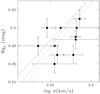 |
Fig. 1 Log σ(km s-1) versus Mg2 diagram based on archival measurements (full squares). Grey lines show the empirical relations for field galaxies (dotted line, Bernardi et al. 1998), and cluster galaxies (Jorgensen et al. 1996; Bernardi et al. 1998, dashed/long-dashed lines, respectively). |
2. The data
Our sample consists of 12 elliptical galaxies with morphological T-type between − 2 and − 5, and recession velocities in the range 2000 ≲ cz ≲ 5500 km s-1, concentrated in the region of the Great Attractor (Lynden-Bell et al. 1988) and mostly belonging to the Centaurus and Hydra clusters. They were all observed between April and June 2000 with the FORS1 camera (0.2″/pix scale, ~7′ × 7′ field of view) at the UT1 unit of the Very Large Telescope – Program Id. 65.O-0073(A), PI R. Scaramella.
Sample of galaxies.
Table 1 lists the objects with some of their properties: besides the coordinates and the colour excess (from Schlegel et al. 1998), we report the morphological T-type, the velocity dispersion σ (km s-1), the Mg2 index, the corrected absolute B-band magnitude (retrieved from the Hyperleda catalogue, Paturel et al. 2003), and the Virgo-infall corrected group velocities, vVirgo, drawn from the NED archive. The table also contains the aperture corrections (see Sect. 2.1) and the total exposure times.
A plot of the Mg2 indices versus the velocity dispersions (Fig. 1) reveals the known mass-metallicity relation (Tremonti et al. 2004; Calura et al. 2009), with more massive objects (larger log σs) that are more metal-rich (larger Mg2s) than others. In the figure we also show the median relations for field (Bernardi et al. 1998) and cluster galaxies (Jorgensen et al. 1996; Bernardi et al. 1998). Although the present sample includes isolated galaxies and galaxies with nearby companions (bright, such as for NGC 5090 and NGC 7117/NGC 7118, or faint companions, such as NGC 6483, NGC 6502, NGC 6987), or objects with possible interactions/merging activity (NGC 5193, NGC 5761), the rms scatter of the residuals for the three plotted relations is ≲0.02, i.e. smaller than, or comparable to, the scatter reported in the quoted papers. As a consequence we can safely assume that the present sample lacks significant peculiarities, which is relevant for the discussion below.
2.1. Data reduction and calibration
The exposures of the 12 ellipticals and the associated calibration frames were retrieved from the ESO archive and processed with standard data reduction procedures using IRAF1 tasks. After bias subtraction and flat-field normalisation, the shifts between single dithered exposures were determined by the shifts of bright, isolated point-like sources. The frames were then summed up adopting a σ-clipping rejection method to remove cosmic-ray hits. No sub-pixel registration was made to avoid the contamination to the SBF caused by the sub-pixel interpolation (Jensen et al. 1998). The resulting images are shown in Fig. 2. The same procedure was carried out for the frames of standard stars. The standard calibration plan of FORS1 provides nightly multi-band observations of Landolt (1992) standards in the high gain mode. However, because the galaxies were observed in low gain mode, 1–3 fields of standard stars per night were collected in this mode as well. We have taken advantage of low/high-gain frames of standard stars to derive the extinction coefficient, kI, whereas the zeropoint was obtained using the low gain frames.
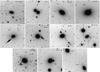 |
Fig. 2 VLT images of the sample galaxies. The objects analysed for SBF measurement appear centred (with the exception of NGC 7117 and NGC 7118) and are labelled in each panel. Each panel shows an area of 300 × 300″, the lower left bar is 20″ long. |
The sample of galaxies was observed in different consecutive runs. The zeropoints, extinction terms, and the IDs of the Landolt (1992) fields of standards are reported in Table 2. The seeing ranged between 0.6″ and 0.8″. Owing to the lack of multi-band observations for the target galaxies, the standard solution of the photometric equations (the photometric calibration that includes both the colour and the atmospheric extinction-correction terms) cannot be applied to the observed galaxies. As a consequence, we derived the solutions of the photometric calibration equations by setting the colour-term coefficients to zero. This forced shortcut, however, does not significantly affect the photometry and the SBF analysis for the following reasons:
-
we compared the calibrated photometry of the sources in the frame of NGC 4696 with the I-band photometry derived by Cantiello et al. (2005) for the same galaxy, based on HST Advanced Camera for Surveys (ACS) observations2. This comparison allows us to reveal any systematic offset in the new photometric data, and/or to unveil possible colour dependencies of the magnitude difference possibly arising from the lack of colour-term correction. The photometry was obtained in both cases with SExtractor (Bertin & Arnouts 1996), as described below in Sect. 2.2. To distinguish between point-sources and extended objects we adopted the SExtractor CLASS_STAR parameter, using CLASS_STAR > 0.7 for good candidate point sources. The results of the comparison are shown in Fig. 3. The two upper panels of the figure show the residuals between the FORS1 and ACS magnitudes for candidate point sources brighter than mI = 24 mag after aperture and extinction correction (the details on the methods used to derive the aperture correction are given in next section). The median difference is consistent with zero. A sizable scatter exists between the two catalogues, which increases with magnitude. This behaviour is not surprising, though, because at fainter magnitudes the star/galaxy classification derived with SExtractor is less reliable. In addition, an excess of negative (mI VLT − mI ACS) values is expected, because of the blending of sources in the lower resolution ground-based images, exemplified in Fig. 4. To emphasise the effects of neglecting the colour term in the photometric calibration of data, the lower panels of Fig. 3 compare the best candidate point sources only (SExtractor star/galaxy classification code: CLASS_STAR > 0.95). The residual differences are still consistent with zero and the scatter, nearly three times smaller than the data shown in the upper panels, is still owing mostly to fainter sources. The flat behaviour of the magnitude difference versus the V − I colour (lower-right panel) shows that neglecting the colour term in the photometric calibration of VLT data affects the magnitudes by less than ~0.05 mag;
-
for the photometric calibration of the nights where V- as well as I-band frames of Landolt standards were available at various air-masses, we obtained V- and I-band colour terms in the range 0.01-0.04, which are typical for FORS13. Adopting a median SBF colour
 mag for galaxies brighter than
MB tot = −20.3 mag (Cantiello et al. 2007a), the expected
colour-correction on
mag for galaxies brighter than
MB tot = −20.3 mag (Cantiello et al. 2007a), the expected
colour-correction on  adopting an I-band colour term
of 0.04 is <0.1 mag4, a relatively small
systematic effect, which will be taken into account in the final error budget; Table 2
adopting an I-band colour term
of 0.04 is <0.1 mag4, a relatively small
systematic effect, which will be taken into account in the final error budget; Table 2Photometric calibration.
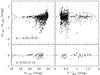
Fig. 3 Upper panels: residuals between VLT and ACS I-band magnitudes versus magnitude (left panel) and colour (right panel). Lower panels: same as the upper panels, but only the best point-source candidates from both catalogues are considered.
-
neglecting the colour-term correction has its greatest effect on the magnitudes of red objects with V − I ≳ 2 mag, i.e. likely background galaxies. These objects – which have a surface density much lower than other sources – are masked out in the SBF measure, because they are a source of unwanted, spurious, fluctuations. In the next section we will discuss the questions related to the masking of the background galaxies in more details as well as those that relate to the estimation of the extra-fluctuation term.
2.2. Data analysis and SBF measurements
Our choice of the images from the VLT programme 65.O-0073(A) was motivated by the need of deep imaging data of galaxies with relatively smooth surface brightness profiles. Before proceeding with the SBF measurements, we checked the expected SBF S/N ratios for the list of galaxies in the programme. In particular, we adopted the inverted relation given by Blakeslee et al. (1999, Eq. (1)): 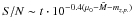 . By using the zero-point magnitudes, mz.p., reported in Table 2, the expected distance moduli from the NED catalogue ( ⟨ μ0 ⟩ column in Table 3), and a fiducial
  mag, we found that in all cases the expected SBF S/N ratio is above the lower limit suggested by Blakeslee et al. (1999), i.e. S/N ≳ 5. The galaxy with the lowest S/N is ESO 322-G101, which has S/N ~ 5. Therefore we proceeded in running the SBF analysis procedure on all sources. A posteriori we rejected one galaxy from the analysis, NGC 5090, a case that will be discussed in the following section. To derive the photometry of the sources and to measure the fluctuation amplitudes in our images we used the same procedure as described in our previous papers (Cantiello et al. 2005, 2007a,b, 2009; Biscardi et al. 2008). The main steps of the SBF measurement contemplate sky background, galaxy modelling and large-scale residual subtraction; photometry and masking of point-like and extended sources and of dust; power-spectrum analysis of the remaining sources in the model-subtracted residual image frame. Here we briefly account for some relevant steps of the analysis, highlighting the differences with previous works where multi-band space-based ACS data were used.
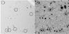 |
Fig. 4 Same 30′ × 30′ region of NGC 4696 as seen by the HST/ACS (left panel) and VLT/FORS1 (right panel) cameras. The circles mark the sources that are blended in the VLT frame. The most severe cases are emphasised with arrows. |
The sky background in the galaxy images was determined by minimising the residuals of the equation I(r) = ISer(r) + Isky, where Isky is the constant sky term, and ISer(r) gives the radial surface brightness profile of the galaxy, μSB(r), assumed to follow Sersic’s law: μSB(r) ∝ − 2.5log ISer(r) or, equivalently, μSB(r) ∝ − r1/n (Sersic 1968; Capaccioli et al. 1995). The procedure of minimisation gave as a result Sersic indices n between 3.5 and 5.5, values typical for the range of the total magnitudes considered (Ferrarese et al. 2006).
After the estimate of the sky background, a first model of the galaxy was obtained and subtracted from the sky-subtracted frame. The wealth of bright sources appearing after the model subtraction and, in some cases, the dust filaments and patches, were masked out. The procedure of model fitting and masking was iteratively repeated until the residual frame (original frame minus sky background and galaxy model) was considered satisfactory. The bright saturated stars in some of the analysed frames (e.g., NGC 4616, NGC 6483) do not represent a major problem in the analysis of the surface brightness profile and the measurement of SBF magnitudes. Indeed, the luminosity profile from which we derive the total magnitudes is analysed using the azimuthal average of the galaxy light-profile. For comparison, the total I-band magnitude estimated by us and by Tonry et al. (2001) for NGC 4616 differs by ~0.15 mag, well within the associated uncertainties (see Sect. 3.1). The main effect of these bright point sources is that a large part of the surrounding area of bright stars have to be masked out to achieve a satisfactory residual frame.
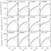 |
Fig. 5 I-band luminosity functions of external sources. The luminosity functions of background galaxies and globular clusters are plotted as dotted and dashed lines, respectively. Open squares mark observational data; the solid lines represent the best fit to the data. |
After subtracting the best galaxy model, the large-scale residuals still present in the frame were removed using the background map obtained with SExtractor adopting a mesh size ~10 times the FWHM (Cantiello et al. 2005).
The photometry of fore/background sources and of the globular clusters in the galaxy was derived with SExtractor from the final residual frame. We modified the input weighting image of SExtractor by adding the galaxy model (times a factor between 0.5 and 2, depending on the galaxy; see Jordán 2004, for details) so that the SBFs were not misinterpreted as real objects. Galactic reddening was corrected using the E(B − V) values from Schlegel et al. (1998) reported in Table 1. The aperture correction (a.c.) was derived selecting a number of isolated point-source candidates in the frames and by making a growth-curve analysis out to 100 pixels diameter, where the contamination by nearby sources is still negligible in the present data (see Stetson 1990, and references therein, for a detailed discussion on the aperture correction for the photometry of point-like sources). The final a.c. values are reported in Table 1.
Once the corrected catalogue of sources was derived, the next step was to fit the luminosity functions of external sources, which were to be used to estimate the extra-fluctuation term, Pr, caused by the unmasked faint sources (see, e.g., Tonry et al. 1990, for more details). We derived the fit to the luminosity functions of the globular clusters and the background galaxies from the photometric catalogues of sources after rejecting the saturated point-like sources (likely foreground stars) and the brightest and most extended objects. The best fit of the sum of the two luminosity functions and the extra-fluctuation correction term Pr were derived as described in Cantiello et al. (2005). The best-fit curves of the total luminosity functions for all galaxies are shown in Fig. 5. We emphasise that the completeness limit for all targets drops significantly at magnitudes fainter than mI ≳ 25 mag. Because the lack of colour information and the lower spatial resolution of these FORS1 compared to ACS data make the distinction between background galaxies and globular clusters less reliable compared to our previous works, we adopted a default uncertainty on the correction δPr = 40%Pr, instead of 25%Pr (Tonry et al. 1990; Cantiello et al. 2005, 2007b). As in Cantiello et al. (2007a), we carried out various numerical tests to verify the robustness of the Pr correction by changing the luminosity function fitting parameters and the source-detection parameters. As a result we found that the effect on the final SBF magnitudes is ≤ 0.2 mag in all cases. Moreover, as an indirect proof of the robustness of the Pr correction estimates, we will show in the following sections the excellent agreement within associated total uncertainties between our present and previous estimates of for NGC 4696.
We estimated the azimuthal average of the residual frame power spectrum, P(k), to measure the SBF magnitudes and matched it with the power spectrum E(k) obtained from a template PSF convolved with the same mask image used for the residual frame. The total fluctuation amplitude P0 was derived via a robust minimisation method (Press et al. 1992), as the multiplicative factor best matching P(k) = P0 × E(k) + P1, where P1 is the white noise constant term (Tonry & Schneider 1988). For each galaxy we used 8 to 14 different isolated bright stars (mI ~ 18 mag) as template PSF, taken from the residual frame. These PSF stars were individually adopted after normalisation to estimate the fluctuation signal of the galaxy. Moreover, the rms between different P0 evaluations obtained with each PSF was included in the error budget of the measure.
For all targets the fluctuation amplitude, Pf = P0 − Pr, was estimated within a circular annulus out to radii where the SBF S/N ratio, given by the ratio Pf/P1 (Tonry & Schneider 1988; Mei et al. 2001), was > 5. In all cases, the S/N in the innermost galaxy regions, i.e. R ≃ 25″, is higher than 50. In general, the ratio of the residual fluctuation to the total fluctuation amplitude was ≲ 30%. The final SBF measures used for distance estimates (Sect. 3.1) are reported in Table 3 together with the statistical and systematic errors – the first includes the error propagation from Pf and Pr, while the latter includes the uncertainty from the photometric zeropoint and the PSF (Cantiello et al. 2005; Blakeslee et al. 2009).
Furthermore, to study the radial variation of SBFs, we ran the measurement procedure in different concentric annuli for each galaxy out to the radius where the SBF exceeds the Pr correction term. The results of this analysis will be discussed in Sect. 4.
SBF data and distances.
3. SBF distances form the fluctuation star count
3.1. Distances based on the  versus
  calibration
As anticipated in Sect. 1, the use of SBF magnitudes as distance indicator relies on existing calibrations, either empirical or theoretical, of the absolute versus the galaxy colour, with V − I being the most commonly used colour. The lack of colour information in the present observational dataset prevents us from using the standard SBF versus colour calibration, which relies on self-consistent colour and SBF measurements. However, Tonry et al. provided an additional way to calibrate SBF magnitudes based on the “fluctuation star count” . This quantity is defined as the difference between the fluctuation magnitude and the total magnitude of the galaxy in a given band  , and corresponds to “ + 2.5log 10 of the total luminosity of the galaxy in units of the luminosity of a typical giant star” (Tonry et al. 2001). By analysing the dependence of on the apparent SBF magnitude in eight groups of galaxies, Tonry et al. found that
  . Another analysis on this distance-independent quantity has been carried out recently by Blakeslee et al. (2009), who derived a calibration of the fluctuation count from z-band SBF measurements of the Virgo and Fornax clusters of galaxies. By comparing the
  versus
  with the versus (g − z) calibration, Blakeslee et al. reported a 2/3 larger scatter of the former calibration. In addition to the larger intrinsic scatter, the dependence of on stellar population properties or, more generally, on the properties of the host galaxy, is not as well-studied as for the colour. Moreover, as discussed by Blakeslee et al. (2009), the versus calibration “no longer has a pure basis in stellar population properties, but rather brings in a scaling relation between galaxy luminosity and colour”, thus, it has the characteristic of a global scaling relation rather than a local relation between the unresolved stellar system and the fluctuation amplitude. As an example, Fig. 6 in Tonry et al. (2001) shows a tight correlation between and the central velocity dispersion of the galaxy. A similar diagram for the present dataset is shown in Fig. 6, the dashed line in the figure shows the best-fit line by Tonry et al. (2001) obtained from a set of ~ 65 galaxies. Notwithstanding the intrinsic physical difference that appears to exist between the
  versus V − I and versus
  calibrations, the fluctuation star count could offer a simple way to derive reliable distances without any colour information, which makes the present sample of measurements adequate for distance determinations and a useful test-case for future applications.
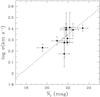 |
Fig. 6 Velocity dispersion versus the fluctuation star count |
For our I-band measurements we adopted the calibration Eq. (4) given by Tonry et al. (2001) – a choice supported also by the agreement between the present dataset and the linear fit to the Tonry and collaborators data shown in Fig. 6 –, changing the zero point as described in Jensen et al. (2003) after the revised Cepheid distances. The final calibration we adopted is  .
.
We used the surface brightness profiles fits described in Sect. 2.2 to derive the total galaxy magnitudes, mItot, needed to evaluate . The corrected total magnitudes are reported in the third column of Table 3. For the objects in common with Tonry et al. (2001), the agreement between the two mItot measures is better than ~ 0.2 mag, with our measures systematically brighter than in Tonry et al. (2001), an effect possibly related to the fact that the SBF-survey by Tonry et al. is based on observations taken with 1.5 m to 4 m-class telescopes, while the present dataset relies upon 8 m class telescope data, which allow for a better sampling of the faint tails of the surface brightness profiles of these bright galaxies. The agreement is worse if the total corrected I-band magnitudes are taken from the Hyperleda catalogue, with the differences increasing to a median ΔmItot ≲ 0.5 mag. For this reason we chose to attach a fixed 0.5 mag uncertainty to our estimates of mItot, which translates into a further 0.07 mag statistical component of the error on the distance moduli. Other sources of uncertainty come from the slope and zero point of the  versus
  calibration. We assume the same uncertainty for the zero-point as that given by Tonry et al. (2001) for the versus V − I calibration, i.e. 0.08 mag. Furthermore, because Tonry et al. do not provide any uncertainty for the slope we decided to adopt a default 20% uncertainty for the error on the slope of the relation (for comparison, the slope of the versus colour relation has ~ 5% error).
Coupling the measured fluctuation amplitudes, the total I-band magnitudes, and the calibration given above, we obtained the distance moduli reported in Table 3. The table also gives the mean, minimum, maximum and group distance moduli for each galaxy, obtained using various distance indicators: Dn − σ, fundamental plane, Tully-Fisher relation, and globular cluster luminosity function (data taken from NED database; see Jacoby et al. 1992, for a critical review on the cited distance indicators).
In general we find that the distances obtained using the calibration agree relatively well with estimates available in literature, showing a median ~0.2 mag difference between our and the literature distance moduli. If single objects are taken into account, though, various considerations can be made. Let us first consider NGC 4696. Cantiello et al. (2005) obtained an SBF-based distance for this galaxy using ACS I-band SBF data and using an independent calibration of the absolute SBF magnitude from the B − I colour (see Cantiello et al. 2005, for details). The distance modulus derived was μ0 = 33.0 ± 0.1 mag, to be compared with the present μ0 = 32.95 ± 0.18(stat.) ± 0.06(sys.) reported in Table 3. The two estimates agree very well, especially if one takes into account that they are completely independent in terms of the fluctuation magnitude measurements (different observational datasets), and considering the calibration used ( versus V − I SBF calibrations). In the following section we will also discuss and compare the SBF radial profiles derived for the two datasets.
For the other galaxies, our distance moduli agree with the estimates found in the literature within the quoted uncertainties. The sole exception is represented by NGC 5090, while NGC 5761 and NGC 7117/NGC 7118 are worth to be discussed in more detail. Our distance modulus for NGC 5090 is μ0 ~ 31.8 mag, nearly ~1.5 mag brighter than the average literature value. This galaxy has a bright foreground companion, the nearly edge-on spiral NGC 5091 visible in Fig. 2. The ~1 mag brighter than expected SBF magnitude is most likely explained by the presence of this bright late-type companion, which also badly affects the estimate of the galaxy total magnitude. As a consequence, we consider the SBF measure of this galaxy and its associated distance to be unreliable, and reject them from the subsequent analysis.
Our distance modulus of NGC 5761 is on average ~0.7 mag fainter than the literature values. The possible explanation for this discrepancy might be the ongoing merging activity of this galaxy, clearly manifested by the stream connecting this galaxy with its companion ESO580-G038. The merging with a lower-mass companion could increase the metal-poor stellar component of the dominating galaxy, inducing brighter SBF magnitudes and bluer integrated colours with respect to similar, but “quiet”, galaxies. A secondary effect of merging on the fluctuation amplitude might come from the morphological distortion caused by the interaction. Indeed, then the luminosity fluctuations between adjacent regions of the galaxy are not dominated anymore by the Poissonian fluctuation of the star counts because the dynamical effects, which are associated with the merging, alter the surface brightness profile introducing a further correlation between adjacent regions. A final possibility, though, is that the sole other measure of μ0 for this galaxy (obtained by Willick et al. 1997, using the Dn − σ relation) is underestimated, which would render any comparison with our estimated distance unreliable. In conclusion we mark NGC 5761 as peculiar and suggest that new distance determinations, obtained using independent distance indicators, are required to provide a final answer to the distance of this galaxy.
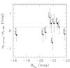 |
Fig. 7 Comparison between SBF distance moduli from this work and group distance moduli derived from the literature. The dashed line shows the median of the residual differences. |
The literature μ0 for NGC 7117/NGC 7118 (Dn − σ estimates from Willick et al. 1997) assumes that the two galaxies share the same distance. Our distance modulus for NGC 7118 is, instead, ~0.3 mag larger than NGC 7117 (~15% nearer in distance). The relatively small angular separation of ~330″ between the two galaxies cannot be considered as a possible source of bias in the SBF measures, because the largest annulus adopted in our measures is <80″ (see Fig. 9 discussed in the next section). Interestingly, a similar ~10% difference between the two μ0 values could also be supported by the recession velocities of the two galaxies (Virgo-infall corrected velocities v = 5422, and 4986 km s-1 for NGC 7117 and NGC 7118, respectively).
The above considerations remain valid if one takes into account the group distance moduli. In particular, our group distance modulus for the three Centaurus cluster members (ESO 322-G101, NGC 4645, and NGC 4696) is μ0 ~ 32.9 mag, versus μ0 ~ 32.8 mag derived from the literature data. A comparison between our distances and group distance moduli shows an average difference of ~0.2 mag (Fig. 7). This difference is within the quoted statistical and systematic uncertainties, especially if one takes into account the other sources of error not included in Table 3, i.e. i) the <0.1 mag error from the neglected colour-term correction (Sect. 2.1), and ii) the ~0.1 mag term owing to the Cepheid’s zero-point uncertainty in the calibration (Freedman & Madore 2010). However, we point out that this offset might be an evidence that the applied calibration is not appropriate, at least for the present sample, and suggests that additional efforts should be made to improve the precision of the calibration.
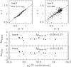 |
Fig. 8 Upper panels: V − I versus B − V relations derived from the SPoT models (left panel Raimondo et al. 2005, models are shown with crosses), and from the integrated colours of Virgo cluster galaxies (right panel). The linear fit to models is shown with dashed line. Lower panels: difference between the distance moduli obtained using the SBF calibration from the V − I colour and from the |
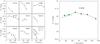 |
Fig. 9 Left panel: SBF magnitudes measured in different galactic annuli versus the mean radius of the annulus. Right panel: SBF versus radius for NGC 4696 as measured from VLT (black squares) and ACS (full triangles, green line) images. The plotted error bars refer to the sole statistical errors. [See electronic version of the Journal for a colour version of the figure.] |
3.2. Comparison with the  versus V − I calibration
In the previous section we have adopted the absolute SBF magnitudes from the calibration to derive distances, rather than the usual versus V − I calibration. In this section we carry out a counter-check of the distances using the standard SBF calibration based on the V − I colour.
To overcome the lack of reliable and homogeneous estimates of the V − I colour we take advantage of the integrated B − V colour available from the Hyperleda database, and transform this colour into V − I . This operation must be carried out with caution, because it has several limitations that have to be properly accounted for: i) the uncertainties of the B − V into V − I colour transformation equations, ii) the intrinsic error of the B − Vmeasurement adopted, and iii) that the integrated colour taken from the literature has likely been measured in regions slightly different from the ones considered in this work.
To transform the B − V into V − I we adopted two different schemes.
-
Case A: we used the simple stellar population models by the Teramo SPoT group (Raimondo et al. 2005)5, fitting a straight line to the B − V and V − I of models with ages between 1 and 14 Gyr and metallicity [Fe/H] between − 1.8 and +0.3 dex. The models and the fit are shown in the upper-left panel of Fig. 8.
-
Case B: we obtained the B − V and V − I colours of the galaxies in the Virgo Cluster Catalogue (VCC, Binggeli et al. 1985) from the Hyperleda archive and fitted a linear relation between the two colours, shown in the upper-right panel of Fig. 8.
![Mathematical equation: \hbox{$\bar{M_I}=-1.58+4.5\cdot[(V-I)-1.15]$}](/articles/aa/full_html/2011/10/aa15670-10/aa15670-10-eq113.png) . We note that the V − I colour obtained lie in all cases in the range of validity of the calibration, i.e. 1.0 ≤ V − I ≤ 1.3 mag.
. We note that the V − I colour obtained lie in all cases in the range of validity of the calibration, i.e. 1.0 ≤ V − I ≤ 1.3 mag.
With this approach we find that the distance moduli derived using the V − I or the calibration differ for ~0.3 mag at most, with a median difference between the distance moduli derived with the colour calibration, μ0, col., and those based on the calibration,  , of
, of  mag if the SPoT colour transformations are used, or
  mag if the observational colour transformations are used. The lower panels in Fig. 8 show the results of these differences. Consequently – even within the non-negligible limitations of the approach proposed in this section – the results of the comparison between the calibrated distances and the V − I calibrated ones show that the distances obtained using the fluctuation star count are consistent with the distances derived with the widely tested SBF-colour calibration.
4. Stellar population analysis from SBF radial profiles
The measurement of SBF magnitudes in different galaxy regions, coupled with stellar population models, has proven to be capable of revealing how stellar population properties change along the distance from the centre of a galaxy (Sodemann & Thomsen 1995; Tonry et al. 2001; Cantiello et al. 2005, 2007a,b, 2011). For the present dataset we analysed the radial profiles of SBF magnitudes. Figure 9 shows for each galaxy the measured SBF per annulus versus the average annulus radius. For ESO 322-G101 we did not succeed in measuring SBF with the required constraint of S/N > 5 in more than one annulus; the case of NGC 5090 is not shown for the reasons explained in Sect. 3.1. A zoom of the NGC 4696 data is shown in the right panel of Fig. 9 where the previous SBF radial gradients measured from ACS data are also shown6. The agreement between the two independent measures is excellent if one takes into account the systematic uncertainties. The difference between the two set of SBF measurements indeed never exceeds ~0.1 mag. Furthermore, a peculiar and unexpected feature in the radial profile of NGC 4696 is the inversion of the SBF versus radius trend at r ≳ 60″, a feature also observed in other objects of the dataset (left panels in Fig. 9).
Previous SBF-gradient analyses have shown that SBF magnitudes become brighter at large galactocentric radii. In a first approximation the negative SBF gradients can be easily associated to a lower average metallicity of field stars at larger radii (Cantiello et al. 2005). Indeed, lower [Fe/H] values imply brighter SBF magnitudes, at least in the I-band (Cantiello et al. 2003). This behaviour is observed in the inner regions of NGC 4696 and, similarly, in NGC 5193, NGC 6502, NGC 6987, and possibly NGC 71187.
However, the presence of a significant positive radial SBF gradient at the farthest galactocentric distances was somehow unexpected. To verify whether this effect is caused by some bias in the data or in the data analysis, we checked the results of the measurements by various tests on the procedure, e.g. by changing the smoothing mesh size of SExtractor, the fitting parameters of the luminosity functions, the parameters used in the procedure to estimate the sky background, the detection/masking of faint sources. All tests confirmed the observed fainter SBF magnitudes at larger radii, leading us to conclude that this is a real property of the present dataset.
Because all galaxies lie at different distances, we assume distances derived from the Virgo-infall corrected group velocities to compare the observed radial SBF gradients in an absolute radial distance scale instead of the radial angular scale shown in Fig. 9, adopting H0 = 73 km s-1 Mpc-1 (e.g. Blakeslee et al. 2002; Riess et al. 2005). Figure 10 shows the SBF gradients in an absolute radius scale.
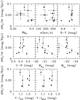 |
Fig. 11 Amplitude of the SBF gradients as a function of various galaxy properties. |
We compared the radial SBF gradients with several observational characteristics of the galaxies to further ascertain if the observed turn-over of the SBF magnitudes is a spurious systematic effect caused by unaccounted factors and not a real feature related to some physical phenomenon acting at large radii. The amplitude of gradients was calculated using a linear fit to the data in Fig. 10, excluding the innermost annuli with negative gradients. In Fig. 11 we plot the gradients against the Mg2 index, the velocity dispersion, the B − V and U − B colours, and the total absolute B and I magnitudes of the galaxies. We also plot the amplitude of gradients versus the V − I colour as derived from the B − V colour using both the empirical and the theoretical B − V to V − I transformations described in Sect. 3.2. For comparison, a similar diagram is shown in Fig. 12, but the absolute SBF magnitudes are plotted instead of the amplitude of gradients. The distances are based on H0 = 73 km s-1 Mpc-1 and on the Virgo-infall-corrected group velocities, to obtain an independent estimate of from μ0. Figure 12 shows some expected correlations, such as the fainter SBF magnitudes for more metal-rich and brighter objects ( versus Mg2 and versus total magnitudes, respectively). Furthermore, a possible correlation with colours seems to be present as well, with SBF magnitudes appearing fainter for objects with larger (redder) B − V , U − B and V − I colours. Indeed, this behaviour is a predictable consequence of the correlation already shown in Fig. 1, i.e. that the metal content of the galaxy scales with its mass – more massive galaxies have deeper potential wells, implying more effective self-enrichment of heavy elements – together with the fact that optical SBF magnitudes become fainter for more metal-rich populations, because, in first approximation the red giant branch becomes fainter and redder (Worthey 1993; Buzzoni 1993; Sodemann & Thomsen 1995). In conclusion, the trends observed in Fig. 12 are mostly an effect of the correlation between the galaxy mass and its host stellar component, and between the latter with SBF magnitudes.
By inspecting Fig. 11 some of the correlations previously discussed seem to be still present. Within the statistical limits of the sample, the relationship of SBF gradients with Mg2 and the total absolute magnitudes is recognisable in the panels of Fig. 11 (shown with linear fits in the respective panels), while the correspondence with colours and velocity dispersion is less obvious. The observed trends point towards steeper positive SBF radial gradients for less massive galaxies, which are characterised by lower Mg2 and fainter total magnitudes. Assuming that this behaviour is real, it could be an indication of the dominating formation activity of the galaxy. More massive galaxies are indeed expected to have a stronger merging activity compared to less massive objects, so that the stellar population gradients, fossils of the proto-cloud collapse stage, are swiped out (see La Barbera et al. 2005, and references therein). As a consequence, one would expect a correlation between the amplitude of SBF gradients and galaxy mass. The results shown in Fig. 11 seem to support this scenario. As explained above, however, the expected correlation should have the opposite sign, that is steeper negative SBF gradients for less massive galaxies, because the mean metallicity of the population should on average decrease at larger galactocentric radii (La Barbera et al. 2005).
A possible alternative explanation might be that the observed positive gradients are linked to an age effect. Keeping the mean metallicity of the stellar populations nearly constant – a reasonable assumption for populations at large radii –, an increase of the mean age with radius would generate fainter SBF magnitudes. As an example, for a drastic and highly unlikely change of age from ~3 Gyr in the inner galactic regions to ~14 Gyr in the outer fields, stellar population synthesis models predict variations of the order of ~0.5 mag for I-band SBF (Blakeslee et al. 2001b; Raimondo et al. 2005). However, some of the cases considered here show up to ~1 mag fainter SBF at large radii, a change that is definitely too drastic to be simply accounted for by an age effect, even for the unrealistically large age gap considered above.
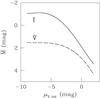 |
Fig. 13 SBF predictions from the SPoT simple stellar population models versus the median V-band magnitude of each model. V and I-band models are shown with different line types, as labelled. |
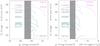 |
Fig. 14 Left panel: SBF magnitudes (plus an arbitrary shift) as a function of the mean surface brightness of the annulus. The grey shaded area marks the region of the |

A different possibly associated effect might be the statistic of the small number of (bright) stars per resolution element at large radii. As shown by Raimondo et al. (2005) using the SPoT stellar population synthesis code, fewer bright stars “per simulation”, or, in the observational case, “per resolution element”, imply fainter SBF magnitudes at a fixed age and metallicity. This behaviour is also exemplified in Fig. 13 for a simple stellar population with an age of 14 Gyr and solar chemical composition8. In the figure we show both V and I-band predictions based on SPoT models (see Sect. 3 in Raimondo et al. 2005, for the details on models and SBF calculation). If the cause of the observed gradients is the statistics of bright stars, model predictions show that this effect is wavelength dependent and stronger at longer wavelengths, possibly owing to the dominant role of bright red-giant branch stars in this regime (see also Cerviño et al. 2008, and references therein). The observational analogue of Fig. 13 is shown in Fig. 14, where we plot the observed SBF gradients versus the apparent and absolute surface brightness profiles for each target galaxy. The qualitative agreement between the models and data in Figs. 13, 14 is probably an indication that the statistics of bright stars might be one of the mechanisms that generate the observed trends. Note that the change of the SBF versus radius slope is observed in Fig. 14 at μI ~ 21 mag/arcsec2, or at an absolute surface brightness of ~−12.5 mag/arcsec2, corresponding to a total absolute magnitude MV ~ −8 mag per resolution element (assuming V − I ~ 1 mag).
Even though specific simulations for different age and metallicity need to be done, the Raimondo et al. simulations show that, below a certain critical luminosity/mass of the stellar population, SBF magnitudes tend to be systematically fainter for fainter total magnitudes, and that the SBF variations predicted by stellar population models are of the order of ~1 mag for a change of total magnitude ~2 mag below a critical limit (see Fig. 2 in Raimondo et al. 2005). If this is the case, then i) the positive SBF gradients at large radii shown in Figs. 9, 10 might have a statistical origin, possibly combined with other effects such as radial age variations, and ii) the steeper SBF gradients for less massive galaxies (Fig. 11) are likely caused by to the more rapid drop of the surface brightness profile below the mentioned critical magnitude for these galaxies.
Although the amplitude of the positive SBF gradients appears to be correlated to the properties of the target galaxies, we must emphasise that the present data and the available models cannot provide a definitive answer in favour of or against the real existence of this feature, or on its possible origin. Future more refined data and models are needed to solve the present puzzle.
5. Summary and conclusions
We measured I-band SBF magnitudes for 12 elliptical galaxies with observations available from the ESO archive, taken with the FORS1 camera at the VLT. The VLT observations were carried out without any additional filter coverage, which prevented the standard use of SBF magnitudes as a distance indicator based on self-consistent SBF and colour measures. Typical applications of the SBF method rely on the knowledge of some integrated colour of the target galaxy, which is used in the calibration of the absolute SBF magnitude – via, e.g., the versus V − I calibration equations. Although few other studies have derived SBF magnitudes based on single-band data (e.g. Sodemann & Thomsen 1995), these applications indeed did use some colour information to obtain the absolute SBF magnitude.
To avoid the uncertainties related to the adoption of a colour from other independent datasets, we carried out an SBF analysis of distances and stellar population properties using the only I-band data (the very first case in the literature, to the best of our knowledge). To derive distances, we estimated the absolute SBF magnitudes using the fluctuation star count, , and adopting the -versus-, calibration provided by Tonry et al. (2001) with an updated zero-point term from Jensen et al. (2003). With the exception of NGC 5090, whose SBF signal is likely contaminated by the light of the foreground companion NGC 5091, we derived distance moduli for all other objects. In general, our distance moduli agree within ~0.2 mag with literature data. In particular, we discussed the case of NGC 4696 for which the present SBF distance (and inner radial SBF gradients) agrees with the estimate by Cantiello et al. (2005) and with other estimates based on different indicators (e.g. Willick et al. 1997; Blakeslee et al. 2001a). The obtained distances have an average statistical uncertainty Δμ0(stat.) ~ 0.2 mag, including the calibration error and the SBF measurement error, and a systematic error Δμ0(sys.) ≲ 0.1 mag, which includes the uncertainty of the photometric zero-point and the PSF scatter. Other components of the systematic error are a <0.1 mag related to the neglected colour-term correction, and a ~0.1 mag term from the Cepheid’s zero-point uncertainty. Adding in quadrature these sources of systematic errors, we obtain an upper limit for the total systematic uncertainty of ~0.2 mag.
In conclusion, apart from some peculiar cases, the comparison between the distances obtained in this work and other estimates shows that the calibration based on can be considered to be reliable and, consequently, even observational datasets based on deep single-band imaging data can be used to derive accurate SBF distances. Hoverer, a systematic difference with literature distances, of the order of the estimated total systematic error ~0.2 mag, seems to be present, suggesting that additional efforts should be made to improve the precision of the calibration.
As for the distances, the potential of SBF as a tracer of stellar population properties relies on the use multi-band SBF data and integrated colours. Nonetheless, for most of the targets it was possible to measure SBF radial variations, and to use these SBF gradients to explore the galaxy properties. For some galaxies we confirmed the existence of negative SBF gradients in the inner galactic regions (r ≲ 10 kpc), a behaviour already observed in other objects (e.g. Cantiello et al. 2005) that has essentially been interpreted as an effect of the lower average metallicity at larger galactocentric radii. However, somehow unexpectedly, we also found positive SBF gradients at larger radii. While various tests allowed us to rule out the possibility of an artifact caused by the image analysis, yet we cannot exclude some unaccounted observational or data analysis effect at such large radii. The observed positive gradients, though, might represent a real physical feature. The slope of the gradients seems indeed to correlate with the total luminosity, i.e. mass, of the host galaxy, similarly to what is observed for the absolute SBF magnitude . Moreover, fainter fluctuation magnitudes for stellar populations characterised by a decreasing number of (bright) stars were predicted using the SPoT models (Raimondo et al. 2005; Raimondo 2009). Thus, the positive SBF gradients found could be caused by a statistical effect in stellar counts, possibly associated with other physical effects, like older mean ages at larger galactocentric radii. Whether or not this detection is real cannot be decided with the present observational data. However, if this interpretation is correct, stellar population synthesis models predict that the statistical effect of stellar counts should be even more evident in the near-IR wavelength regime. Thus present-day near-IR devices, like HAWK-I at the VLT, or the WFC3/IR channel installed on the HST, will be able to provide a definitive answer to the intriguing behaviour found in these data. This result, if confirmed by independent SBF measurements, will be a fundamental step towards both a better understanding of the SBF method and, even more, a solid agreement about the role played by statistical effects when the surface density of unresolved stellar systems is reasonably low.
IRAF is distributed by the National Optical Astronomy Observatories, which are operated by the Association of Universities for Research in Astronomy, Inc., under cooperative agreement with the National Science Foundation.
Cantiello et al. (2005) transformed the F814W ACS magnitudes into the standard I ones using the Sirianni et al. (2005) transformation equations. The authors quoted a typical correction between the two bands (I − F814W) ~ 0.01 mag.
Historical trends taken from he ESO quality control web pages http://www.eso.org/qc/
The  is ≲ 2.0 mag for fainter galaxies. Thus, for the present sample, the colour correction of ESO 322-G101 should be even smaller.
Teramo SPoT (Stellar POpulation Tools) models are available at the web site www.oa-teramo.inaf.it/spot
For sake of homogeneity we have reanalysed the ACS data using circular instead of elliptical annuli. At a fixed average radius the new SBF measurements agree with previous ones within the associated uncertainties.
We exclude NGC 5761 from the above list because, as discussed in Sect. 3.1, it is quite peculiar compared to the other galaxies.
The adopted stellar population model parameters are not intended to match the real physical age and metallicity of the stellar populations in elliptical galaxies, they are rather indented to show the relative behaviour of a well defined stellar population when the density of stars (thus the associated luminosity) per resolution elements decreases significantly.
Acknowledgments
We thank G. Raimondo for helpful discussions on the effect of the statistics of stellar counts on SBF magnitudes. M. Cantiello acknowledges support from COFIS ASI-INAF I/016/07/0, PRIN-INAF 2008 (PI. M. Marconi), and MIUR-FIRB 2008 (PI. G. Imriani). This research made use of the NASA/IPAC Extragalactic Database (NED) which is operated by the Jet Propulsion Laboratory, California Institute of Technology, under contract with NASA. We acknowledge the use of the HyperLeda database. Based on data obtained from the ESO Science Archive Facility under requests number cantiell129537-cantiell129720.
References
- Ajhar, E. A., & Tonry, J. L. 1994, ApJ, 429, 557 [NASA ADS] [CrossRef] [Google Scholar]
- Bekki, K., & Shioya, Y. 2001, Ap&SS, 276, 767 [NASA ADS] [CrossRef] [Google Scholar]
- Bernardi, M., Renzini, A., da Costa, L. N., et al. 1998, ApJ, 508, L143 [Google Scholar]
- Bertin, E., & Arnouts, S. 1996, A&AS, 117, 393 [NASA ADS] [CrossRef] [EDP Sciences] [Google Scholar]
- Binggeli, B., Sandage, A., & Tammann, G. A. 1985, AJ, 90, 1681 [NASA ADS] [CrossRef] [Google Scholar]
- Biscardi, I., Raimondo, G., Cantiello, M., & Brocato, E. 2008, ApJ, 678, 168 [NASA ADS] [CrossRef] [Google Scholar]
- Blakeslee, J. P., Ajhar, E. A., & Tonry, J. L. 1999, in Post-Hipparcos cosmic candles, ASSL, 237, 181 [NASA ADS] [Google Scholar]
- Blakeslee, J. P., Lucey, J. R., Barris, B. J., Hudson, M. J., & Tonry, J. L. 2001a, MNRAS, 327, 1004 [NASA ADS] [CrossRef] [Google Scholar]
- Blakeslee, J. P., Vazdekis, A., & Ajhar, E. A. 2001b, MNRAS, 320, 193 [NASA ADS] [CrossRef] [Google Scholar]
- Blakeslee, J. P., Lucey, J. R., Tonry, J. L., et al. 2002, MNRAS, 330, 443 [NASA ADS] [CrossRef] [Google Scholar]
- Blakeslee, J. P., Jordán, A., Mei, S., et al. 2009, ApJ, 694, 556 [NASA ADS] [CrossRef] [Google Scholar]
- Buzzoni, A. 1993, A&A, 275, 433 [NASA ADS] [Google Scholar]
- Calura, F., Pipino, A., Chiappini, C., Matteucci, F., & Maiolino, R. 2009, A&A, 504, 373 [NASA ADS] [CrossRef] [EDP Sciences] [Google Scholar]
- Cantiello, M., Raimondo, G., Brocato, E., & Capaccioli, M. 2003, AJ, 125, 2783 [NASA ADS] [CrossRef] [Google Scholar]
- Cantiello, M., Blakeslee, J. P., Raimondo, G., et al. 2005, ApJ, 634, 239 [NASA ADS] [CrossRef] [Google Scholar]
- Cantiello, M., Blakeslee, J., Raimondo, G., Brocato, E., & Capaccioli, M. 2007a, ApJ, 668, 130 [NASA ADS] [CrossRef] [Google Scholar]
- Cantiello, M., Raimondo, G., Blakeslee, J. P., Brocato, E., & Capaccioli, M. 2007b, ApJ, 662, 940 [NASA ADS] [CrossRef] [Google Scholar]
- Cantiello, M., Raimondo, G., Brocato, E., & Biscardi, I. 2009, Mem. Soc. Astron. Ital., 80, 40 [NASA ADS] [Google Scholar]
- Cantiello, M., Biscardi, I., Brocato, E., & Raimondo, G. 2011, A&A, 532, 154 [Google Scholar]
- Capaccioli, M., D’Onofrio, M., & Caon, N. 1995, Astrophys. Lett. Commun., 31, 169 [NASA ADS] [Google Scholar]
- Carlberg, R. G. 1984, ApJ, 286, 403 [NASA ADS] [CrossRef] [Google Scholar]
- Cerviño, M., Luridiana, V., & Jamet, L. 2008, A&A, 491, 693 [NASA ADS] [CrossRef] [EDP Sciences] [Google Scholar]
- Davies, R. L., Sadler, E. M., & Peletier, R. F. 1993, MNRAS, 262, 650 [NASA ADS] [Google Scholar]
- Faber, S. M., Wegner, G., Burstein, D., et al. 1989, ApJS, 69, 763 [NASA ADS] [CrossRef] [Google Scholar]
- Ferrarese, L., Côté, P., Jordán, A., et al. 2006, ApJS, 164, 334 [NASA ADS] [CrossRef] [Google Scholar]
- Foster, C., Proctor, R. N., Forbes, D. A., et al. 2009, MNRAS, 400, 2135 [NASA ADS] [CrossRef] [Google Scholar]
- Freedman, W. L., & Madore, B. F. 2010, ARA&A, 48, 673 [NASA ADS] [CrossRef] [Google Scholar]
- Fritz, A. 2002, Baltic Astron., 11, 385 [NASA ADS] [Google Scholar]
- Jacoby, G. H., Branch, D., Ciardullo, R., et al. 1992, PASP, 104, 599 [NASA ADS] [CrossRef] [Google Scholar]
- Jensen, J. B., Luppino, G. A., & Tonry, J. L. 1996, ApJ, 468, 519 [NASA ADS] [CrossRef] [Google Scholar]
- Jensen, J. B., Tonry, J. L., & Luppino, G. A. 1998, ApJ, 505, 111 [NASA ADS] [CrossRef] [Google Scholar]
- Jensen, J. B., Tonry, J. L., Barris, B. J., et al. 2003, ApJ, 583, 712 [Google Scholar]
- Jordán, A. 2004, ApJ, 613, L117 [NASA ADS] [CrossRef] [Google Scholar]
- Jorgensen, I., Franx, M., & Kjaergaard, P. 1996, MNRAS, 280, 167 [NASA ADS] [CrossRef] [Google Scholar]
- Kampakoglou, M., Trotta, R., & Silk, J. 2008, MNRAS, 384, 1414 [NASA ADS] [CrossRef] [Google Scholar]
- Kauffmann, G., White, S. D. M., & Guiderdoni, B. 1993, MNRAS, 264, 201 [NASA ADS] [CrossRef] [Google Scholar]
- La Barbera, F., Merluzzi, P., Busarello, G., Massarotti, M., & Mercurio, A. 2004, A&A, 425, 797 [NASA ADS] [CrossRef] [EDP Sciences] [Google Scholar]
- La Barbera, F., de Carvalho, R. R., Gal, R. R., et al. 2005, ApJ, 626, L19 [NASA ADS] [CrossRef] [Google Scholar]
- Landolt, A. U. 1992, AJ, 104, 340 [NASA ADS] [CrossRef] [Google Scholar]
- Lorenz, H., Bohm, P., Capaccioli, M., Richter, G. M., & Longo, G. 1993, A&A, 277, L15 [NASA ADS] [Google Scholar]
- Lynden-Bell, D., Faber, S. M., Burstein, D., et al. 1988, ApJ, 326, 19 [NASA ADS] [CrossRef] [Google Scholar]
- Mei, S., Quinn, P. J., & Silva, D. R. 2001, A&A, 371, 779 [NASA ADS] [CrossRef] [EDP Sciences] [Google Scholar]
- O’Connell, R. W. 1986, in Stellar Populations, ed. C. A. Norman, A. Renzini, & M. Tosi, 167 [Google Scholar]
- Pahre, M. A., & Mould, J. R. 1994, ApJ, 433, 567 [NASA ADS] [CrossRef] [Google Scholar]
- Paturel, G., Petit, C., Prugniel, P., et al. 2003, A&A, 412, 45 [NASA ADS] [CrossRef] [EDP Sciences] [Google Scholar]
- Press, W. H., Teukolsky, S. A., Vetterling, W. T., & Flannery, B. P. 1992, Numerical recipes in FORTRAN, The art of scientific computing, 2nd edn. (Cambridge: University Press) [Google Scholar]
- Raimondo, G. 2009, ApJ, 700, 1247 [NASA ADS] [CrossRef] [Google Scholar]
- Raimondo, G., Brocato, E., Cantiello, M., & Capaccioli, M. 2005, AJ, 130, 2625 [NASA ADS] [CrossRef] [Google Scholar]
- Riess, A. G., Li, W., Stetson, P. B., et al. 2005, ApJ, 627, 579 [NASA ADS] [CrossRef] [Google Scholar]
- Schlegel, D. J., Finkbeiner, D. P., & Davis, M. 1998, ApJ, 500, 525 [NASA ADS] [CrossRef] [Google Scholar]
- Sersic, J. L. 1968, Atlas de galaxias australes (Cordoba, Argentina: Observatorio Astronomico) [Google Scholar]
- Sirianni, M., Jee, M. J., Benítez, N., et al. 2005, PASP, 117, 1049 [NASA ADS] [CrossRef] [Google Scholar]
- Sodemann, M., & Thomsen, B. 1995, AJ, 110, 179 [NASA ADS] [CrossRef] [Google Scholar]
- Spolaor, M., Proctor, R. N., Forbes, D. A., & Couch, W. J. 2009, ApJ, 691, L138 [NASA ADS] [CrossRef] [Google Scholar]
- Stetson, P. B. 1990, PASP, 102, 932 [NASA ADS] [CrossRef] [Google Scholar]
- Tonry, J. L. 1991, ApJ, 373, L1 [NASA ADS] [CrossRef] [Google Scholar]
- Tonry, J., & Schneider, D. P. 1988, AJ, 96, 807 [NASA ADS] [CrossRef] [Google Scholar]
- Tonry, J. L., Ajhar, E. A., & Luppino, G. A. 1990, AJ, 100, 1416 [NASA ADS] [CrossRef] [Google Scholar]
- Tonry, J. L., Dressler, A., Blakeslee, J. P., et al. 2001, ApJ, 546, 681 [NASA ADS] [CrossRef] [Google Scholar]
- Tremonti, C. A., Heckman, T. M., Kauffmann, G., et al. 2004, ApJ, 613, 898 [NASA ADS] [CrossRef] [Google Scholar]
- Willick, J. A., Courteau, S., Faber, S. M., et al. 1997, ApJS, 109, 333 [NASA ADS] [CrossRef] [Google Scholar]
- Willmer, C. N. A., Maia, M. A. G., Mendes, S. O., et al. 1999, AJ, 118, 1131 [Google Scholar]
- Worthey, G. 1993, ApJ, 409, 530 [NASA ADS] [CrossRef] [Google Scholar]
- Worthey, G. 1994, ApJS, 95, 107 [NASA ADS] [CrossRef] [Google Scholar]
All Tables
All Figures
|
Fig. 1 Log σ(km s-1) versus Mg2 diagram based on archival measurements (full squares). Grey lines show the empirical relations for field galaxies (dotted line, Bernardi et al. 1998), and cluster galaxies (Jorgensen et al. 1996; Bernardi et al. 1998, dashed/long-dashed lines, respectively). |
| In the text | |
|
Fig. 2 VLT images of the sample galaxies. The objects analysed for SBF measurement appear centred (with the exception of NGC 7117 and NGC 7118) and are labelled in each panel. Each panel shows an area of 300 × 300″, the lower left bar is 20″ long. |
| In the text | |
|
Fig. 3 Upper panels: residuals between VLT and ACS I-band magnitudes versus magnitude (left panel) and colour (right panel). Lower panels: same as the upper panels, but only the best point-source candidates from both catalogues are considered. |
| In the text | |
|
Fig. 4 Same 30′ × 30′ region of NGC 4696 as seen by the HST/ACS (left panel) and VLT/FORS1 (right panel) cameras. The circles mark the sources that are blended in the VLT frame. The most severe cases are emphasised with arrows. |
| In the text | |
|
Fig. 5 I-band luminosity functions of external sources. The luminosity functions of background galaxies and globular clusters are plotted as dotted and dashed lines, respectively. Open squares mark observational data; the solid lines represent the best fit to the data. |
| In the text | |
|
Fig. 6 Velocity dispersion versus the fluctuation star count |
| In the text | |
|
Fig. 7 Comparison between SBF distance moduli from this work and group distance moduli derived from the literature. The dashed line shows the median of the residual differences. |
| In the text | |
|
Fig. 8 Upper panels: V − I versus B − V relations derived from the SPoT models (left panel Raimondo et al. 2005, models are shown with crosses), and from the integrated colours of Virgo cluster galaxies (right panel). The linear fit to models is shown with dashed line. Lower panels: difference between the distance moduli obtained using the SBF calibration from the V − I colour and from the |
| In the text | |
|
Fig. 9 Left panel: SBF magnitudes measured in different galactic annuli versus the mean radius of the annulus. Right panel: SBF versus radius for NGC 4696 as measured from VLT (black squares) and ACS (full triangles, green line) images. The plotted error bars refer to the sole statistical errors. [See electronic version of the Journal for a colour version of the figure.] |
| In the text | |
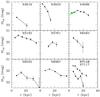 |
Fig. 10 As in Fig. 9, but versus the absolute radius in kpc. |
| In the text | |
|
Fig. 11 Amplitude of the SBF gradients as a function of various galaxy properties. |
| In the text | |
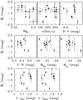 |
Fig. 12 As in Fig. 11, but absolute SBF magnitudes are plotted instead of SBF gradients. |
| In the text | |
|
Fig. 13 SBF predictions from the SPoT simple stellar population models versus the median V-band magnitude of each model. V and I-band models are shown with different line types, as labelled. |
| In the text | |
|
Fig. 14 Left panel: SBF magnitudes (plus an arbitrary shift) as a function of the mean surface brightness of the annulus. The grey shaded area marks the region of the |
| In the text | |
Current usage metrics show cumulative count of Article Views (full-text article views including HTML views, PDF and ePub downloads, according to the available data) and Abstracts Views on Vision4Press platform.
Data correspond to usage on the plateform after 2015. The current usage metrics is available 48-96 hours after online publication and is updated daily on week days.
Initial download of the metrics may take a while.