| Issue |
A&A
Volume 533, September 2011
|
|
|---|---|---|
| Article Number | A26 | |
| Number of page(s) | 17 | |
| Section | Astronomical instrumentation | |
| DOI | https://doi.org/10.1051/0004-6361/201117337 | |
| Published online | 22 August 2011 | |
Circular polarization measurement in millimeter-wavelength spectral-line VLBI observations
1
Department of Astronomy and Institute for Advanced Computing Applications
and Technologies, University of Illinois at Urbana-Champaign,
1002 W. Green Street,
Urbana,
IL,
61801
USA
e-mail: This email address is being protected from spambots. You need JavaScript enabled to view it.
2 Department of Physics and Electronics, Rhodes University, PO
Box 94, Grahamstown, 6140, South Africa
Received:
24
May
2011
Accepted:
23
June
2011
Abstract
This paper considers the problem of accurate measurement of circular polarization in imaging spectral-line VLBI observations in the λ = 7 mm and λ = 3 mm wavelength bands. This capability is especially valuable for the full observational study of compact, polarized SiO maser components in the near-circumstellar environment of late-type, evolved stars. Circular VLBI polarimetry provides important constraints on SiO maser astrophysics, including the theory of polarized maser emission transport, and on the strength and distribution of the stellar magnetic field and its dynamical role in this critical circumstellar region. We perform an analysis here of the data model containing the instrumental factors that limit the accuracy of circular polarization measurements in such observations, and present a corresponding data reduction algorithm for their correction. The algorithm is an enhancement of existing spectral line VLBI polarimetry methods using autocorrelation data for calibration, but with innovations in bandpass determination, autocorrelation polarization self-calibration, and general optimizations for the case of low SNR, as applicable at these wavelengths. We present an example data reduction at λ = 7 mm and derive an estimate of the predicted accuracy of the method of mc ≤ 0.5% or better at λ = 7 mm and mc ≤ 0.5−1% or better at λ = 3 mm. Both the strengths and weaknesses of the proposed algorithm are discussed, along with suggestions for future work.
Key words: masers / techniques: interferometric / techniques: polarimetric / stars: AGB and post-AGB
© ESO, 2011
1. Introduction
SiO maser emission acts as an important tracer of the astrophysical conditions in the near-circumstellar environments of late-type, evolved stars (Habing 1996). The maser emission is detected in vibrationally-excited, rotational molecular transitions of SiO, denoted ν = ν′, J = J′ − (J′ − 1), which have rest frequencies of order ν0 ~ 43J′ GHz. Commonly, the brightest and most frequently observed lines are the ν = 1, J = 1−0 and ν = 1, J = 2−1 transitions near 43 GHz and 86 GHz respectively.
In single-dish observations, the SiO maser emission from late-type, evolved stars shows an
appreciable degree of linear polarization: ml ~ 15−30%, or
greater (Troland et al. 1979), but a significantly
lower degree of circular polarization, with typical median values
mc ~ several percent (Barvainis et al. 1987). In a single-dish survey of SiO linear polarization
variability in evolved stars, Glenn et al. (2003)
report a mean sample linear polarization  with a dispersion of 7%. A larger single-dish survey of late-type, evolved stars in full
polarization by Herpin et al. (2006) was able to
classify mean polarization by stellar type or variability class. They report
with a dispersion of 7%. A larger single-dish survey of late-type, evolved stars in full
polarization by Herpin et al. (2006) was able to
classify mean polarization by stellar type or variability class. They report
 and
and  for Mira variables,
  and
and  for semi-regular variables, and
  and
and  for supergiant stars. Overall, the measured single-dish values are consistent with
theoretical expectations, given the non-paramagnetic nature of the SiO molecule and the
associated general theory of the propagation of polarized maser emission in the limit of
small Zeeman splitting (Goldreich et al. 1973).
for supergiant stars. Overall, the measured single-dish values are consistent with
theoretical expectations, given the non-paramagnetic nature of the SiO molecule and the
associated general theory of the propagation of polarized maser emission in the limit of
small Zeeman splitting (Goldreich et al. 1973).
Radio-interferometric observations of SiO maser emission toward late-type, evolved stars can measure the radiation properties of the SiO maser emission at high angular resolution in the full set of Stokes parameters {I,Q,U,V}. For Very Long Baseline Interferometry (VLBI), this angular resolution is at the sub-milliarcsecond (mas) level, and is sufficient to resolve individual SiO maser components. However, the low level of mean circular SiO maser polarization, and the intrinsic millimeter observing wavelengths required for these transitions, pose challenges in Stokes V instrumental calibration of VLBI observations of SiO masers. Measurements of SiO maser circular polarization at mas angular resolution are important however, both to constrain theoretical models describing the propagation of polarized maser emission, and for the subsequent application of these theories to infer the magnitude and orientation of the underlying magnetic fields from measurements of component-level SiO maser polarization properties. Recently, for example, periodic changes in single-dish fractional circular polarization have been detected toward two SiO stars (Wiesemeyer et al. 2009), with a proposed explanation that these changes are tracing precessing planetary magnetospheres in the circumstellar environment (Wiesemeyer 2009).
In this paper we consider the instrumental factors that constrain measurements of SiO circular polarization using VLBI arrays, evaluate the degree to which these effects can be calibrated and corrected, and provide an assessment of the net accuracy of SiO circular polarization observations at 43 GHz and 86 GHz.
The development and first application of VLBI polarimetry was reported by Cotton et al. (1984) and Wardle et al. (1986). It has since grown to become a mature technique, of broad applicability; see Cawthorne et al. (1993) and Pollack et al. (2003) for example. For the frequency bands considered in the current paper, the first continuum polarization VLBI were reported at 43 GHz by Kemball et al. (1996), and at 86 GHz by Attridge (2001).
These prior works were concerned with linear polarimetry of continuum extra-galactic radio
sources. Homan & Wardle (1999) developed a
method to allow circular VLBI polarimetry of continuum sources however, by assuming a source
ensemble has  ;
this technique has been demonstrated successfully at wavelengths longer than
λ ≥ 1 cm (Homan et al. 2009), and
is discussed in further detail below. The first spectral-line polarimetry in full
Stokes {I,Q,U,V} at 43 GHz – of the
ν = 1,J = 1−0 SiO maser emission toward the Mira
variable, TX Cam – was reported by Kemball & Diamond
(1997), based on technical development described earlier by Kemball et al. (1995). Critical circular spectral-line VLBI polarimetry
of water masers in the adjacent 22 GHz band was succesfully performed by Vlemmings et al. (2002) following this same method.
;
this technique has been demonstrated successfully at wavelengths longer than
λ ≥ 1 cm (Homan et al. 2009), and
is discussed in further detail below. The first spectral-line polarimetry in full
Stokes {I,Q,U,V} at 43 GHz – of the
ν = 1,J = 1−0 SiO maser emission toward the Mira
variable, TX Cam – was reported by Kemball & Diamond
(1997), based on technical development described earlier by Kemball et al. (1995). Critical circular spectral-line VLBI polarimetry
of water masers in the adjacent 22 GHz band was succesfully performed by Vlemmings et al. (2002) following this same method.
The current paper examines the sources of instrumental and propagation errors in VLBI circular polarimetry in the λ = 7 mm and λ = 3 mm bands in more detail, and develops and tests refinements to existing calibration methods to improve the accuracy to which Stokes V and mc can be measured in such observations. We show that it is possible to refine existing calibration methods based on autocorrelation data that avoid the need for amplitude self-calibration. We demonstrate these refinements on an observed dataset, and show that an error in mc of ≤ 0.5% or better is possible in practice at λ = 7 mm and mc ≤ 0.5−1% or better at λ = 3 mm.
The paper is structured as follows: Sect. 2 describes the instrumental and propagation data model, and Sect. 3 discusses the associated data reduction methods. The analysis of a test dataset is described in Sect. 4. General discussion and conclusions are presented in Sects. 5 and 6 respectively.
2. Theory
This section describes the data model, containing propagation and instrumental effects relevant to precise amplitude calibration of millimeter-wavelength spectral-line VLBI observations.
Given the focus of the paper described in the Introduction, this discussion is confined primarily to the case of the VLBA1 operating at observing frequencies of 43 GHz (λ = 7 mm) and 86 GHz (λ = 3 mm). However, these techniques are broadly applicable to spectral-line VLBI observations at millimeter wavelengths in general. Implicit to this discussion are the instrumental parameters applicable to the VLBA; these are summarized in Table 1, individually referenced as indicated from Romney (2010) or Napier (1995). For each of the two observing bands considered here, the table contains columns summarizing the receiver band frequency limits, adopted center frequency, typical zenith system equivalent flux density (SEFD), primary beam angular full-width half-maximum θb, typical root-mean-square (rms) pointing error σp, beam squint separation △ s, and the typical baseband bandwidth assigned to an individual maser transition at these observing frequencies. The beam squint results from the offset Cassegrain optics adopted in the VLBA antenna design (Napier 1995). We note also that each of these VLBA bands is dual polarization, with nominal orthogonal RCP and LCP polarization receptors.
VLBA system parameters at millimeter wavelengths.
2.1. Data model
The data model includes all propagation and instrumental calibration effects in the signal path from the frame of the astronomical source to the correlator output. Kemball et al. (1995) present a signal-path analysis of this type for spectral line polarization VLBI in general. We extend this formalism here to include a more detailed assessment of the problem of amplitude calibration for millimeter observing wavelengths in the case of low, but non-zero, Stokes V. For brevity, we use the same notation as the original paper by Kemball et al. (1995) wherever possible, and enumerate only the data model differences here. These are presented in the same approximate sequential order in which they appear in the signal path.
Kemball et al. (1995) presented a reduction heuristic for spectral line polarization VLBI observations for the case where no prior assumption can be made concerning the magnitude of Stokes V. In contrast for example, in continuum VLBI polarimetry of compact, extra-galactic sources, the approximation Stokes V ~ 0 can be applied during data reduction to a relatively high degree of accuracy. The approach described by Kemball et al. (1995) defines a data model and develops a full calibration solution in amplitude, phase, group delay, and fringe rate for a reference receptor polarization p ∈ {R,L} using standard single-polarization VLBI techniques; and then defines a method to tie that solution to the calibration solution for the orthogonal receptor polarization q by solving for and applying differential polarization offsets in amplitude, phase, and group delay. We retain that methodology here, but focus specifically on total and differential polarization amplitude calibration, and its role in precise Stokes V measurement at millimeter wavelengths. This discussion includes a deeper examination of the data model for autocorrelation data specifically, given their relevance to amplitude calibration for spectral line VLBI observations as approached here.
2.2. General
We carry over several general assumptions made in Kemball et al. (1995) to the current analysis. Given the small angular size of astrophysical maser regions observed with VLBI and the millimeter observing wavelengths considered here, the interferometric image formation problem is in the narrow-field regime. No correction is required for the non-coplanar baselines effect in image formation, and all image-plane calibration effects can be treated as visibility-plane calibration effects. All calibration terms are factorized accordingly as antenna-based. We adopt a dual-circular orthogonal polarization basis ((p,q) ∈ {R,L}), in keeping with our instrumental focus on the VLBA.
2.3. Atmosphere
Ionospheric Faraday rotation (IFR) produces a differential polarization phase offset
 ,
where ν is the observing frequency. Using a maximum daytime IFR estimated
in Thompson et al. (2001) from Evans & Hagfors (1968) to be 15 rotations at
ν = 100 MHz for a line-of-sight at a zenith angle
z = 60°, we predict approximate IFR values of
γR−L ~ 0.03° and
γR−L ~ 0.007° at 43 GHz
and 86 GHz respectively, consistent with intuitive expectations. This effect can therefore
be ignored in the current analysis:
γR−L ≪ 1°.
,
where ν is the observing frequency. Using a maximum daytime IFR estimated
in Thompson et al. (2001) from Evans & Hagfors (1968) to be 15 rotations at
ν = 100 MHz for a line-of-sight at a zenith angle
z = 60°, we predict approximate IFR values of
γR−L ~ 0.03° and
γR−L ~ 0.007° at 43 GHz
and 86 GHz respectively, consistent with intuitive expectations. This effect can therefore
be ignored in the current analysis:
γR−L ≪ 1°.
The troposphere is non-dispersive and produces no differential polarization calibration offsets in any of the calibration quantities. However, the time-variable water vapor and dry atmosphere constituents are major contributors to absorption in the millimeter-wavelength bands considered here. We regard the atmosphere as isothermal, with temperature Tatm. For an atmospheric line of sight of optical depth τ, the noise power contribution from the isothermal atmosphere is (1 − e−τ) Tatm.
2.4. Image-plane effects
As noted above, the narrow-field constraint applicable in this case (and in most standard VLBI observations) allows relevant image-plane effects to be factorized as antenna-based corrections in the visibility plane. This does not detract from the origin of these effects in the image plane however. For the observing wavelengths and specific instrumental emphasis considered here, the most important image-plane effects originate from antenna pointing errors. These pointing errors change the region of the antenna primary beam located toward the angular direction of the correlated field center. This causes variation in the calibration terms that vary with angular separation from the optical center of the antenna primary beam, such as the amplitude and polarization response.
The nominal pointing performance and beam squint of the VLBA antennas at these observing
wavelengths are summarized in Table 1. In the
presence of pointing errors, the VLBA primary beam squint (△ s ~ 5% of
θ) introduces a differential polarization amplitude error. This problem
can be analyzed in one dimension without loss of generality. We model the one-dimensional
normalized primary beam power pattern at each antenna along angular axis
ζ as a Gaussian function of width θ, beam squint
△ s, and pointing error ϵp, for nominal
orthogonal receptor polarizations (p,q) ∈ {R,L} as:
 The
differential polarization amplitude error in this model takes the form:
The
differential polarization amplitude error in this model takes the form:  (3)The
R/L amplitude ratio at the nominal
pointing position ζ = 0 is plotted as a function of pointing error
ϵp in Fig. 1, for beam
squint
(3)The
R/L amplitude ratio at the nominal
pointing position ζ = 0 is plotted as a function of pointing error
ϵp in Fig. 1, for beam
squint  , as
applicable to the VLBA.
, as
applicable to the VLBA.
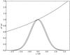 |
Fig. 1 Plot of normalized primary beam patterns in 1-d cross-section for receptor
polarizations {R,L} with a beam squint equal to 5% of the
full-width at half-maximum θb; the
x-ordinate for the beam pattern plot is in units of
θb. The ratio of the two beam
patterns is also plotted in the upper part of the diagram as a function of pointing
error ϵp, with x-ordinate
|

This effect is clearly significant for the representative pointing rms values enumerated in Table 1 for the VLBA operating at these observing wavelengths. We discuss calibration methods for this effect in the second half of this paper.
The net instrumental polarization response at each antenna in each nominal circular receptor polarization (p,q) ∈ {R,L} can be parametrized in terms of the net receptor ellipticity and orientation or equivalently as a complex D-term representing the net leakage of unwanted signal from the orthogonal nominal polarization (Conway & Kronberg 1969). The net instrumental polarization response contains contributions from the antenna optics design, feed illumination function, polarizer performance, and to a lesser extent, other electronic components in the downstream signal path that have a differential polarization response. The net instrumental polarization is an image-plane (direction-dependent) effect but, in the current narrow-field scientific application, we again factorize it as an antenna-based visibility plane correction factor, in common with the other image-plane calibration effects considered in this section. Pointing errors introduce time-variability in the net instrumental polarization response, expressed as an antenna-based visibility plane correction, by sampling different regions of the primary beam polarization pattern, a contributor to the net D-term. The associated dependence on frequency is neglected here due to the small fractional bandwidth.
2.5. Total power
Total power relationships for single-dish telescopes are discussed by Kutner & Ulich (1981), Downes (1989), and Wilson et al.
(2009). Adapting this references, we represent the total system temperature at an
individual antenna in nominal receptor polarization p in the form:
 where
where
 is the amplitude loss for an
angular pointing error ϵp, the term
is the amplitude loss for an
angular pointing error ϵp, the term
 is the source
Rayleigh-Jeans brightness temperature (radiation temperature) in receptor polarization
p, ηl includes antenna scattering and
antenna resistive (ohmic) losses,
τ = τ(z) is the optical depth along
the line of sight at zenith angle z through the atmosphere,
Tspill is the mean ground spill-over temperature,
is the source
Rayleigh-Jeans brightness temperature (radiation temperature) in receptor polarization
p, ηl includes antenna scattering and
antenna resistive (ohmic) losses,
τ = τ(z) is the optical depth along
the line of sight at zenith angle z through the atmosphere,
Tspill is the mean ground spill-over temperature,
 is the net
receiver temperature in receptor polarization p, and
Tatm is the mean temperature of the isothermal atmosphere
along the line of sight.
is the net
receiver temperature in receptor polarization p, and
Tatm is the mean temperature of the isothermal atmosphere
along the line of sight.
2.6. Autocorrelation and cross-power spectra
Autocorrelation and cross-power spectra are formed by interferometric correlation of all
polarization pairs for the voltages recorded in each nominal receptor polarization at each
antenna in the array. We assume idealized analog correlation here for clarity but without
loss of generality – the effects of quantization, sampling, and other digital signal
processing effects are considered in subsequent sections. Following the notation of Kemball et al. (1995), we denote the normalized
autocorrelation and cross-power spectra as
 and
and
 respectively
for antenna indices (m,n) and nominal receptor polarizations
(p,q). The spectra are normalized by the geometric mean of the total
power in the signal received at each antenna (m,n) forming part of the
correlation pair.
respectively
for antenna indices (m,n) and nominal receptor polarizations
(p,q). The spectra are normalized by the geometric mean of the total
power in the signal received at each antenna (m,n) forming part of the
correlation pair.
In this section we express the data model for
and
in the more
modern measurement equation (ME) matrix formalism introduced by Hamaker et al. (1996) and Sault et al.
(1996).
2.6.1. Autocorrelation data model
We denote the normalized analog autocorrelation spectrum as a 4-vector
 ; this is
real-valued for polarization p = q and complex for
p ≠ q.
; this is
real-valued for polarization p = q and complex for
p ≠ q.
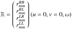 (6)where
(u,v) are visibility-plane coordinates and ω denotes
angular frequency. We denote the true source correlation spectrum as J. In the
autocorrelation case, this is the (antenna-independent) source total-power spectrum,
(6)where
(u,v) are visibility-plane coordinates and ω denotes
angular frequency. We denote the true source correlation spectrum as J. In the
autocorrelation case, this is the (antenna-independent) source total-power spectrum,
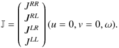 (7)We denote a
total-power noise term contribution
(7)We denote a
total-power noise term contribution 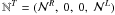 ,
where
,
where  . Following Kemball et al. (1995), we use
 to denote
the point-source sensitivity (in Jy/K) of antenna m in receptor
polarization p. The total system temperature at antenna
m in polarization p is denoted as
to denote
the point-source sensitivity (in Jy/K) of antenna m in receptor
polarization p. The total system temperature at antenna
m in polarization p is denoted as
 and
follows Eq. (5).
and
follows Eq. (5).
The autocorrelation data model can then be represented in matrix form as, 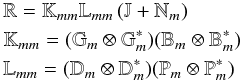 (8)where
⊗ denotes an outer matrix product, and
Gm,Bm,Dm
and Pm are 2 × 2 Jones matrices denoting gain normalization,
complex bandpass response, instrumental polarization, and parallactic angle feed
rotation respectively. This follows the measurement equation formalism of Hamaker et al. (1996) but includes a self-noise term,
as required in the autocorrelation data model considered here. In this
circularly-polarized basis, the Jones matrices take the form,
(8)where
⊗ denotes an outer matrix product, and
Gm,Bm,Dm
and Pm are 2 × 2 Jones matrices denoting gain normalization,
complex bandpass response, instrumental polarization, and parallactic angle feed
rotation respectively. This follows the measurement equation formalism of Hamaker et al. (1996) but includes a self-noise term,
as required in the autocorrelation data model considered here. In this
circularly-polarized basis, the Jones matrices take the form, 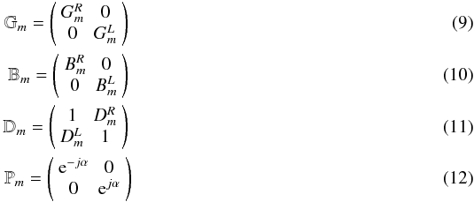 Kmm
is a therefore a diagonal 4 × 4 matrix containing the gain normalization
Kmm
is a therefore a diagonal 4 × 4 matrix containing the gain normalization
 and complex
bandpass response terms
and complex
bandpass response terms  ,
, 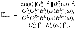 (13)The
net instrumental polarization response Lmm including D-terms
and parallactic angle rotation is the 4 × 4 matrix,
(13)The
net instrumental polarization response Lmm including D-terms
and parallactic angle rotation is the 4 × 4 matrix,  (14)
(14)
2.6.2. Cross-correlation data model
The cross-correlation data model does not include a self-noise term; in this case
Eq. (8) takes the form,  (15)where
X is a diagonal 4 × 4 matrix term for cross-correlation coherence losses; this term does
not apply to autocorrelation data. X does not contribute to differential polarization
amplitude offsets, and forms part of the calibration of the absolute flux density scale.
(15)where
X is a diagonal 4 × 4 matrix term for cross-correlation coherence losses; this term does
not apply to autocorrelation data. X does not contribute to differential polarization
amplitude offsets, and forms part of the calibration of the absolute flux density scale.
Here, Jmn is the true source visibility cross-power
spectrum,  (16)as a function of
(u,v)-spacing and frequency ω.
(16)as a function of
(u,v)-spacing and frequency ω.
2.7. Sampling and quantization
The voltages in each nominal receptor polarization are digitally sampled and quantized by
the data acquisition sub-systems at each antenna. Digital realizations
 of the
total-power and cross-power spectra are obtained by subsequent cross-correlation. We
denote the relationship between the measured spectra
and their
true analog counterparts used in
earlier sections as a general transformation function
fd:
of the
total-power and cross-power spectra are obtained by subsequent cross-correlation. We
denote the relationship between the measured spectra
and their
true analog counterparts used in
earlier sections as a general transformation function
fd:  The
form of this relationship depends on quantization level, sampler voltage threshold
stability and accuracy, and correlator architecture, and is reviewed by Thompson et al. (2001) and references therein. This
transformation function does not always take closed analytic form.
The
form of this relationship depends on quantization level, sampler voltage threshold
stability and accuracy, and correlator architecture, and is reviewed by Thompson et al. (2001) and references therein. This
transformation function does not always take closed analytic form.
The specific case of sampling and quantization effects for the VLBA correlator is considered by Kogan (1998). This correlator has an FX architecture, originally hardware-based but more recently upgraded to a VLBA-DiFX software implementation (Deller et al. 2007). Both one- and two-bit sampling are supported. An offset in sampler threshold voltage can produce an associated amplitude error in the output VLBA correlator spectra (Kogan 1998), particularly for two-bit sampling. If the mapping of individual sampler modules to sets of baseband converters mirrors receptor polarization baseband assignment – as occurs naturally for several common baseband converter configurations – these amplitude offsets will translate to differential polarization amplitude errors. The correction of quantization and sampler threshold errors is discussed in further detail in the following section.
3. Data reduction methods
In this section we assess the data reduction methods used to measure and correct the instrumental and propagation terms in the data model enumerated in Sect. 2. Consistent with earlier practice, we describe here only differences with the data reduction methodology presented by Kemball et al. (1995) and use identical notation wherever possible. This section follows the proposed data reduction sequence, which is shown in flowchart form in Fig. 2.
We have implemented these algorithms within a development framework that brings together several large community codes used for radio-astronomical imaging (Kemball et al. 2008). For consistency with earlier algorithmic work in Kemball et al. (1995) we have primarily used an adapted implementation of the Astronomical Image Processing System2 within this software framework for the current work. Our intention is to make these revisions publicly available in the future.
 |
Fig. 2 Flowchart depicting the overall data reduction sequence described in Sect. 3. |
3.1. Sampling and quantization
In this section, we review the correction of digital sampling and quantization effects in VLBI circular polarimetry at millimeter wavelengths. We do not find it necessary to revise existing algorithmic practice, as described in the analysis below.
The total-power and cross-power spectra from the
VLBA FX correlator are first corrected for quantization effects and then scaled in
amplitude by polarization-independent factors known a-priori for the array (the latter
known historically as b-factors). The quantization correction element of the
transformation function fd defined in
Sect. 2.7 above is defined as a relation for each quantization mode (one- or two-bit,
ηQ = 11 or
ηQ = 22 respectively) between a measured
correlation ρm and the true underlying
correlation ρ, both defined in the conjugate Fourier delay lag domain. In
lag space, the correlation is of order  for cross-power spectra; for the VLBA system temperatures listed in Table 1 and for typical SiO maser spectral flux densities,
lag-domain correlation values are small
|ρm| ≲ 0.1. In this case, the relation
between ρm and ρ is in the
highly linear regime (Kogan 1998) and the
quantization correction can be applied as a direct linear scaling of cross-power spectral
values
for cross-power spectra; for the VLBA system temperatures listed in Table 1 and for typical SiO maser spectral flux densities,
lag-domain correlation values are small
|ρm| ≲ 0.1. In this case, the relation
between ρm and ρ is in the
highly linear regime (Kogan 1998) and the
quantization correction can be applied as a direct linear scaling of cross-power spectral
values  with numerical
coefficient αQ (Kogan 1993a). As this takes the form of a linear,
polarization-independent correction, it cannot produce an artificial instrumental
signature mimicking Stokes V. Cross-polarized autocorrelation spectra
with numerical
coefficient αQ (Kogan 1993a). As this takes the form of a linear,
polarization-independent correction, it cannot produce an artificial instrumental
signature mimicking Stokes V. Cross-polarized autocorrelation spectra
 have
lag domain correlation values of order
have
lag domain correlation values of order  ,
as indicated by the first-order form of Eq. (8), and similarly fall in the low-correlation regime. Accordingly they have the
same quantization scaling correction as cross-power spectra.
,
as indicated by the first-order form of Eq. (8), and similarly fall in the low-correlation regime. Accordingly they have the
same quantization scaling correction as cross-power spectra.
Parallel-hand autocorrelation spectra  have lag-domain correlation
values of unity at zero delay, and require Fourier transformation to and from the lag
domain to allow application of the full non-linear correction between
ρm and ρ (Kogan 1993a). As a result, this does not reduce to a
linear scaling relationship for the total-power spectra
in the
frequency domain. Two effects limit the accuracy of the inverse transform to the lag
domain. The VLBA FX correlator records only positive spectral channels (Kogan 1993a), omitting the opposite sideband which
contains digitization noise (Thompson et al. 2001).
In addition, an FX correlator requires equal-length zero padding to reconstruct the
associated correlation function over the full range of sampled delay lags (Granlund 1986; Thompson
et al. 2001).
have lag-domain correlation
values of unity at zero delay, and require Fourier transformation to and from the lag
domain to allow application of the full non-linear correction between
ρm and ρ (Kogan 1993a). As a result, this does not reduce to a
linear scaling relationship for the total-power spectra
in the
frequency domain. Two effects limit the accuracy of the inverse transform to the lag
domain. The VLBA FX correlator records only positive spectral channels (Kogan 1993a), omitting the opposite sideband which
contains digitization noise (Thompson et al. 2001).
In addition, an FX correlator requires equal-length zero padding to reconstruct the
associated correlation function over the full range of sampled delay lags (Granlund 1986; Thompson
et al. 2001).
Sampler threshold voltages define transition points between discrete quantization states. The non-linear mapping between ρm and ρ depends functionally on the value of the sampler threshold voltages relative to their optimal values (Kogan 1995). For two-bit sampling in the low-correlation limit, the relative error in FX spectral output depends linearly on the deviation in threshold voltage level. In one-bit sampling, the relative error in spectral output depends only in second order on the error in the threshold clipping voltage (Kogan 1995). In both VLBA quantization modes, the correction in output spectral amplitude can be derived from the measured mean deviation of the total-power spectra from the unit mean power level predicted for an ideal digitizer, independent of spectral shape (Kogan 1995), and we adopt that approach here.
The autocorrelation data are used in integrated template-fitting as part of calibration, as described in further detail below.
3.2. Bandpass calibration
Following Kemball et al. (1995), and the Jones
matrix formalism in Eq. (10) in the current
work, we denote the cross-power complex bandpass response as
 ; this is expanded as
 .
The autocorrelation bandpass amplitude response, denoted
.
The autocorrelation bandpass amplitude response, denoted
 , differs from the cross-power
bandpass amplitude response
, differs from the cross-power
bandpass amplitude response  however, due to an unavoidable
level of irreducible aliasing in the net system bandpass response. As the continuum
calibrators have flat spectra across the baseband bandwidth they are used to solve for
and
using cross- and total-power
continuum calibrator data respectively.
however, due to an unavoidable
level of irreducible aliasing in the net system bandpass response. As the continuum
calibrators have flat spectra across the baseband bandwidth they are used to solve for
and
using cross- and total-power
continuum calibrator data respectively.
3.2.1. Bandpass frequency frame
The VLBA correlator produces output cross- and total-power spectra in a geocentric
J2000.0 coordinate reference frame. In contrast, the bandpass response function
is defined in the data
acquisition coordinate reference frame at each antenna, which is an apparent topocentric
frame. These two frequency frames are offset by the time-variable natural geometric
fringe rate at antenna m, denoted
△ ωm(t). The angular
frequency of channel number l in the recorded cross- and total-power
visibility spectra (which are in a geocentric frame) is denoted as
ωl. The autocorrelation bandpass amplitude response
 at
antenna m in receptor polarization
p ∈ {R,L} can be solved for by minimizing:
at
antenna m in receptor polarization
p ∈ {R,L} can be solved for by minimizing:
![Mathematical equation: \begin{eqnarray} \label{bp-ac}\left[\chi^{pp}_m\right]^2 & = &\sum_{k=1}^{N_t}\sum_{l=1}^{N_{\rm c}}\left[\|B_{a,m}^p(\omega_{\rm l}-\triangle \omega_m(t_k))\|^2 - \tilde{V}_{mm}^{pp}\right]^2 \\ \tilde{V}_{mm}^{pp} & = & \|V_{mm}^{pp}(\omega_{\rm l},t_k)\|/\overline{\|V_{mm}^{pp}(\omega_{\rm l},t_k)\|} \end{eqnarray}](/articles/aa/full_html/2011/09/aa17337-11/aa17337-11-eq129.png) where
where
 is the (real-valued)
continuum calibrator total-power spectrum in parallel-hand polarization correlation
pp at antenna m over a pre-average integration
interval centered at time tk, the number of
frequency channels is Nc, and the number of integration
intervals is Nt. The pre-average interval
is fixed and short relative to
is the (real-valued)
continuum calibrator total-power spectrum in parallel-hand polarization correlation
pp at antenna m over a pre-average integration
interval centered at time tk, the number of
frequency channels is Nc, and the number of integration
intervals is Nt. The pre-average interval
is fixed and short relative to  .
Pre-averaging improves the statistical robustness of the bandpass response solver, as
this is a least-squares minimization problem. The autoscaling of each total-power
spectrum by the instantaneous mean spectral amplitude,
.
Pre-averaging improves the statistical robustness of the bandpass response solver, as
this is a least-squares minimization problem. The autoscaling of each total-power
spectrum by the instantaneous mean spectral amplitude,
 ,
ensures that the spectra do not need to be calibrated in amplitude before solving for
. The resulting solution for
is normalized to unit mean
power
,
ensures that the spectra do not need to be calibrated in amplitude before solving for
. The resulting solution for
is normalized to unit mean
power 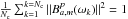 .
.
Bandpass calibration forms part of visibility amplitude calibration and accurate
estimation of Stokes V requires a correspondingly accurate solution for
 . For example, a spurious
bandpass amplitude spike, even if in an off-source spectral region, will bias the mean
amplitude normalization of the bandpass over the region of source emission.
. For example, a spurious
bandpass amplitude spike, even if in an off-source spectral region, will bias the mean
amplitude normalization of the bandpass over the region of source emission.
The measured visibility spectra and the unknown bandpass response are not in a common
frequency frame; the channel shift corresponding to
△ ωm is a non-negligible effect at the
wavelengths of λ = 3 mm and λ = 7 mm considered in
this paper. If is parametrized discretely
as a set of unknown values at each frequency channel (in a stationary topocentric frame)
then this can be estimated by direct integration of the total-power, parallel-hand
spectra if they are first shifted to the stationary reference frame by using a discrete
Fourier transform pair including a channel shift. Alternatively, the unshifted
visibility spectra can be fit directly if is parametrized as a
polynomial series expansion over frequency; this parametrization allows continuous
variation of △ ωm(t) in
the formulation of the chi-square minimization problem. This method was developed by
Kemball & Diamond (1997), using a
Chebyshev polynomial expansion for the bandpass response. The polynomial bandpass method
avoids digital signal processing artifacts associated with the Fourier transform shift.
In addition, as the polynomial expansion order can be significantly lower than the
number of frequency channels Nc, this approach reduces the
number of free parameters over the discrete parametrization case, thus improving the
signal-to-noise ratio (SNR) of the bandpass solution. For these reasons (amongst others
discussed below), we adopt the bandpass polynomial solution method. In a Chebyshev
expansion, the autocorrelation bandpass response takes the form:
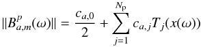 (21)where
Tj(x) is the Chebyshev
polynomial of degree j (Press et al.
2007), ca,j are real coefficients
in the series expansion for the autocorrelation bandpass amplitude, and the transformed
coordinate is
x(ω) = (2ω − ωa − ωb)/(ωb − ωa).
The topocentric channel range for the bandpass solution covered by the measured
visibility spectra is
[ωa = 1 − max(△ ωm), ωb = Nc − min(△ ωm)] .
In the current work, we found it important to fit over the full topocentric range
[ωa,ωb]
as opposed to only [1,Nc] as used in
past practice, so that there is the greatest possible chi-square constraint on the
bandpass solution at the edge of the frequency channel range. The derived solution
coefficients ca,j resulting from the
chi-square minimization over
[ωa,ωb]
are then transformed to
(21)where
Tj(x) is the Chebyshev
polynomial of degree j (Press et al.
2007), ca,j are real coefficients
in the series expansion for the autocorrelation bandpass amplitude, and the transformed
coordinate is
x(ω) = (2ω − ωa − ωb)/(ωb − ωa).
The topocentric channel range for the bandpass solution covered by the measured
visibility spectra is
[ωa = 1 − max(△ ωm), ωb = Nc − min(△ ωm)] .
In the current work, we found it important to fit over the full topocentric range
[ωa,ωb]
as opposed to only [1,Nc] as used in
past practice, so that there is the greatest possible chi-square constraint on the
bandpass solution at the edge of the frequency channel range. The derived solution
coefficients ca,j resulting from the
chi-square minimization over
[ωa,ωb]
are then transformed to  over
[1,Nc] as (Press et al. 2007),
over
[1,Nc] as (Press et al. 2007),  During
this coefficient transformation, if
ωb < Nc
or ωa > 1 then the
outer
During
this coefficient transformation, if
ωb < Nc
or ωa > 1 then the
outer  are
extrapolated horizontally to cover the complete range
[1,Nc] .
are
extrapolated horizontally to cover the complete range
[1,Nc] .
We note that Eq. (19) is formulated for the case of a time-invariant bandpass at each antenna. This is an appropriate instrumental assumption given the expected stability of the net VLBA frequency response, and improves the signal-to-noise ratio of the resulting bandpass solution. In addition a single bandpass solution provides greater control over the calibration of overall differential polarization R/L amplitude and phase offsets.
In the most direct formulation, the cross-power bandpass response
can be solved for from the
parallel-hand continuum calibrator cross-power spectra
 by an
analogous formulation of Eq. (19),
by an
analogous formulation of Eq. (19),
![Mathematical equation: \begin{eqnarray} \left[\chi^{pp}\right]^2 & = & \sum_{m,n>m}^{N_a}\sum_{k=1}^{N_t}\sum_{l=1}^{N_{\rm c}}\left\| B_{m}^p(\omega_{lm})B_{n}^{p*}(\omega_{ln}) -{\tilde{V}^{pp}_{mn}}\right\|^2 \label{bp-xc}\\ \tilde{V}^{pp}_{mn}&=& V_{mn}^{pp}(\omega_{\rm l},t_k)\ /\ {\overline{V_{mn}^{pp}(\omega_{\rm l},t_k)}}\nonumber\\ \omega_{lm} & = & \omega_{\rm l}-\triangle \omega_m(t_k) \nonumber \\ \omega_{ln} & = & \omega_{\rm l}-\triangle \omega_n(t_k) \nonumber \end{eqnarray}](/articles/aa/full_html/2011/09/aa17337-11/aa17337-11-eq155.png) (25)where
(25)where
 is the complex normalization factor to auto-scale the cross-power spectrum in
integration tk over frequency to unit mean
amplitude and zero mean phase. The auto-scaling applied during the chi-square
minimization removes the requirement for amplitude calibration of
is the complex normalization factor to auto-scale the cross-power spectrum in
integration tk over frequency to unit mean
amplitude and zero mean phase. The auto-scaling applied during the chi-square
minimization removes the requirement for amplitude calibration of
 , as in the case for the
autocorrelation bandpass , but for the cross-power
bandpass solution, the visibility data need to be calibrated in the phase domain for
residual group delay, fringe-rate, phase, and differential polarization phase offset, as
described by Kemball et al. (1995). The resulting
solutions for are normalized over
frequency to unit mean power
, as in the case for the
autocorrelation bandpass , but for the cross-power
bandpass solution, the visibility data need to be calibrated in the phase domain for
residual group delay, fringe-rate, phase, and differential polarization phase offset, as
described by Kemball et al. (1995). The resulting
solutions for are normalized over
frequency to unit mean power  and zero mean phase. The
polynomial bandpass method is further favored in the cross-power case as there is no
unique shift defined for
Vmn(tk)
if instead of a polynomial bandpass expansion, the visibility data are shifted using a
Fourier transform.
and zero mean phase. The
polynomial bandpass method is further favored in the cross-power case as there is no
unique shift defined for
Vmn(tk)
if instead of a polynomial bandpass expansion, the visibility data are shifted using a
Fourier transform.
3.2.2. Bandpass aliasing correction
The solutions obtained for the cross-power bandpass response
from the direct formulation
in Eq. (25) are not optimal however for
precise amplitude calibration at the millimeter wavelengths (λ = 3 mm
and λ = 7 mm) considered here. At these wavelengths, the amplitude of
the continuum calibrator cross-power spectra on the longer baselines invariably have
insufficient SNR to allow estimation of with low mean-square error
(MSE) at the outlying antennas. The autocorrelation spectra have significantly higher
SNR however, and offer a preferred path for the solution of the cross-power bandpass
amplitude response if corrected for aliasing, as
found necessary in the current work. We adopt an aliasing model:  (26)where
Ab(ω) is a model for the
cross-power bandpass amplitude response at and above the upper end of the band (in a
frequency range
ωk0 > βωc,
where ωc is the bandpass cutoff frequency and
β lies in the approximate range
β ~ {0.7−0.9}). This function can be extrapolated and folded to
approximate the aliased autocorrelation response. We find a 12-node Butterworth function
(Bianchi & Sorrentino 2007) to give a
satisfactory empirical fit to the upper-bandpass region
ωk0 > βωc,
with little sensitivity to the value of β adopted to define the channel
range of the fit:
(26)where
Ab(ω) is a model for the
cross-power bandpass amplitude response at and above the upper end of the band (in a
frequency range
ωk0 > βωc,
where ωc is the bandpass cutoff frequency and
β lies in the approximate range
β ~ {0.7−0.9}). This function can be extrapolated and folded to
approximate the aliased autocorrelation response. We find a 12-node Butterworth function
(Bianchi & Sorrentino 2007) to give a
satisfactory empirical fit to the upper-bandpass region
ωk0 > βωc,
with little sensitivity to the value of β adopted to define the channel
range of the fit:  (27)The fit minimizes:
![Mathematical equation: \begin{eqnarray} [\chi^{pp}]^2&=&\sum_{k=k0}^{N_{\rm c}}\left[\|B_m^p(\omega_k)\|^2-\left(A_m^p(\omega_k)\right)^2\right]^2\nonumber\\ &&+ \sum_{k=k0}^{N_{\rm c}-1}[\|B_{a,m}^p(\omega_k)\|^2-\|B_m^p(\omega_k)\|^2\nonumber\\ &&\mbox{}- \left(A_m^p(\omega_{(2N_{\rm c}-k)})\right)^2]^2 \end{eqnarray}](/articles/aa/full_html/2011/09/aa17337-11/aa17337-11-eq167.png) (28)where
the number of nodes is fixed at n = 12, and factor a
and the cutoff frequency ωc are the only fitted parameters.
The direct cross-power solutions for obtained from Eq. (25) do however have sufficient SNR to allow
a solution for Ab(ω) in
Butterworth form (27). The solution for
Ab(ω) allows the
high-SNR autocorrelation bandpass amplitude solutions
to be then transformed to
cross-power form:
(28)where
the number of nodes is fixed at n = 12, and factor a
and the cutoff frequency ωc are the only fitted parameters.
The direct cross-power solutions for obtained from Eq. (25) do however have sufficient SNR to allow
a solution for Ab(ω) in
Butterworth form (27). The solution for
Ab(ω) allows the
high-SNR autocorrelation bandpass amplitude solutions
to be then transformed to
cross-power form:  (29)In this hybrid
approach, the phase
(29)In this hybrid
approach, the phase  of the cross-power bandpass
response is solved for by minimizing the phase-only analog of Eq. (25):
of the cross-power bandpass
response is solved for by minimizing the phase-only analog of Eq. (25): ![Mathematical equation: \begin{eqnarray} \left[\chi^{pp}\right]^2 &=&\sum_{m,n>m}^{N_a}\sum_{k=1}^{N_t}\sum_{l=1}^{N_{\rm c}}\big[ \varsigma_{m}^p(\omega_{\rm l}-\triangle \omega_m(t_k))\nonumber\\ && \mbox{} - \varsigma_n^p(\omega_{\rm l}-\triangle \omega_n(t_k))-\arg(\tilde{V}_{mn}^{pp}(\omega_{\rm l},t_k))\big]^2 \label{bp-xcp} \end{eqnarray}](/articles/aa/full_html/2011/09/aa17337-11/aa17337-11-eq172.png) (30)where
(30)where
 are the pre-averaged
continuum calibrator cross-power visibility spectra, normalized to unit mean amplitude
and zero mean phase, and calibrated in delay, fringe-rate, and phase as described above.
In practice, the peak-to-peak residual phase error over frequency for the net VLBA
baseband response after correction for phase and group delay is typically of order 5
degrees, and we fit at each antenna in each
receptor polarization with a low-order polynomial in order to maximize SNR. The complex
cross-power bandpass response is therefore represented by
a separate Chebyshev polynomial in each of amplitude and phase, with a lower-order
polynomial in phase compared to that in amplitude. The final cross-power bandpass
solution is therefore constructed as,
are the pre-averaged
continuum calibrator cross-power visibility spectra, normalized to unit mean amplitude
and zero mean phase, and calibrated in delay, fringe-rate, and phase as described above.
In practice, the peak-to-peak residual phase error over frequency for the net VLBA
baseband response after correction for phase and group delay is typically of order 5
degrees, and we fit at each antenna in each
receptor polarization with a low-order polynomial in order to maximize SNR. The complex
cross-power bandpass response is therefore represented by
a separate Chebyshev polynomial in each of amplitude and phase, with a lower-order
polynomial in phase compared to that in amplitude. The final cross-power bandpass
solution is therefore constructed as,
 (31)applying
the unit-mean power and zero-mean phase normalization to the bandpass solutions as
described above.
(31)applying
the unit-mean power and zero-mean phase normalization to the bandpass solutions as
described above.
3.2.3. Reference antenna differential polarization bandpass phase response
We note that the solution for is derived by solving a
self-calibration problem that is linear in baseline-based phase, and so is known only
relative to the phase at receptor polarization p for an adopted
reference antenna (subscript zero), i.e. the determined bandpass phase solution takes
the form  , as opposed to
, the argument of
, as opposed to
, the argument of
 in the Jones matrix of Eq. (10). A full
solution, allowing correction of cross-polarized visibility spectra therefore requires
an independent estimate of the differential polarization bandpass phase response at the
reference antenna
in the Jones matrix of Eq. (10). A full
solution, allowing correction of cross-polarized visibility spectra therefore requires
an independent estimate of the differential polarization bandpass phase response at the
reference antenna  . This
is directly analogous to the correction of parallel-hand phase solutions for
differential polarization phase and delay offsets at the reference antenna, as described
by Kemball et al. (1995). The correction for
has
not traditionally been applied to bandpass corrections in spectral-line VLBI but is
relevant to the autocorrelation polarimetry described in subsequent sections of this
paper, so was implemented in the current work. Without this correction, for example,
there would be no bandpass phase correction applied to the cross-polarized
autocorrelation spectra at the reference antenna.
. This
is directly analogous to the correction of parallel-hand phase solutions for
differential polarization phase and delay offsets at the reference antenna, as described
by Kemball et al. (1995). The correction for
has
not traditionally been applied to bandpass corrections in spectral-line VLBI but is
relevant to the autocorrelation polarimetry described in subsequent sections of this
paper, so was implemented in the current work. Without this correction, for example,
there would be no bandpass phase correction applied to the cross-polarized
autocorrelation spectra at the reference antenna.
3.2.4. Bandpass correction
The basic algebra for applying the autocorrelation bandpass response
and
to correct the visibility
data is described by Kemball et al. (1995) and
Diamond (1989). These references describe a
traditional  heuristic for autocorrelation bandpass correction, to minimize the residual total-power
offset. However, the complete autocorrelation data model used here (Eq. (8)) does not include this term – nor is it
necessary – so we do not subtract 1 when correcting the autocorrelation bandpass
response in the current work. Additionally, during bandpass application, the fringe-rate
shift is applied when computing the polynomial expansion of
or
.
heuristic for autocorrelation bandpass correction, to minimize the residual total-power
offset. However, the complete autocorrelation data model used here (Eq. (8)) does not include this term – nor is it
necessary – so we do not subtract 1 when correcting the autocorrelation bandpass
response in the current work. Additionally, during bandpass application, the fringe-rate
shift is applied when computing the polynomial expansion of
or
.
3.3. Amplitude calibration
Amplitude calibration of the correlation spectra  in units of spectral flux
density
in units of spectral flux
density  (Jy) requires independent
measurement of the total system temperature (K) and
point-source sensitivity (Jy
K-1) both at each antenna m and in each receptor
polarization p throughout the course of the observation. We denote the
system equivalent flux density (SEFD) as
(Jy) requires independent
measurement of the total system temperature (K) and
point-source sensitivity (Jy
K-1) both at each antenna m and in each receptor
polarization p throughout the course of the observation. We denote the
system equivalent flux density (SEFD) as  (Jy). In
the formalism used in this paper (see Eq. (13) and following),
(Jy). In
the formalism used in this paper (see Eq. (13) and following),  .
The are
time-variable due to changes in both atmospheric attenuation and antenna gravitational
deformation, both as a function of time and antenna pointing position in local horizon
coordinates.
.
The are
time-variable due to changes in both atmospheric attenuation and antenna gravitational
deformation, both as a function of time and antenna pointing position in local horizon
coordinates.
Sections 3.3.1 and 3.3.2 contain a review and analysis of current practice in VLBI continuum and spectral-line amplitude calibration, with a specific focus on circular polarimetry at millimeter wavelengths. We describe the innovations in amplitude calibration introduced in the current work in Sect. 3.3.3.
3.3.1. Continuum amplitude calibration
The VLBA records integrated system temperatures every two minutes at each antenna in
each receptor polarization p ∈ {R,L} obtained
using an underlying switched noise calibration system (Thompson 1995). The VLBA project also publishes opacity-corrected gain curves
for each antenna, which provide  as a
polynomial function of zenith angle z; these curves are obtained from
analyses of regular single-dish service observations, separately scheduled (Walker 1999).
as a
polynomial function of zenith angle z; these curves are obtained from
analyses of regular single-dish service observations, separately scheduled (Walker 1999).
In standard a priori amplitude calibration of VLBI continuum observations, the
 are computed as
 from the measured system temperature values and published antenna point-source
sensitivity curves. At the observing wavelengths λ = 7 mm and
λ = 3 mm considered in this paper the opacity-corrected
provided by the VLBA require correction for atmospheric attenuation
e−τ (Walker
1999; and see Eq. (5)). As
described by Leppänen (1993), these corrections
can be obtained by fitting the measured system temperatures over the course of the
observations as a function of zenith angle z against a simplified form
of Eq. (5):
from the measured system temperature values and published antenna point-source
sensitivity curves. At the observing wavelengths λ = 7 mm and
λ = 3 mm considered in this paper the opacity-corrected
provided by the VLBA require correction for atmospheric attenuation
e−τ (Walker
1999; and see Eq. (5)). As
described by Leppänen (1993), these corrections
can be obtained by fitting the measured system temperatures over the course of the
observations as a function of zenith angle z against a simplified form
of Eq. (5):
 (32)where
 is the
antenna temperature contribution from the source. The number of free parameters can be
controlled by adopting a plane-parallel atmosphere, with
τ = τ0secz for zenith
opacity τ0, extrapolating Tatm
from ground-level metrology, and adopting an empirical model for the spill-over noise
contribution for VLBA antennas (Leppänen 1993).
In this case, only receiver temperature Trx and zenith
opacity τ0 remain as free parameters, and once solved for
using chi-square minimization, allow opacity correction in the form:
is the
antenna temperature contribution from the source. The number of free parameters can be
controlled by adopting a plane-parallel atmosphere, with
τ = τ0secz for zenith
opacity τ0, extrapolating Tatm
from ground-level metrology, and adopting an empirical model for the spill-over noise
contribution for VLBA antennas (Leppänen 1993).
In this case, only receiver temperature Trx and zenith
opacity τ0 remain as free parameters, and once solved for
using chi-square minimization, allow opacity correction in the form:
 The
a priori amplitude calibration methods outlined above are limited in their intrinsic
accuracy by several sources of error. These include systematic errors in the measured or
adopted power level of the noise calibration sources, intrinsic statistical error in the
sampled switched Tsys measurements, and the stability over
time of hardware elements affecting amplitude calibration, including receiver gain and
the stability of the noise calibration sources. In addition, the opacity solution is
limited by the assumption of a stable, plane-parallel atmosphere; this does not hold at
low elevations or if local weather conditions vary significantly over the course of the
observations (i.e.
τ0 = τ0(t)).
Other sources of systematic error include the assumption of an isothermal
Tatm extrapolated from the measured ground air
temperature, and the relatively coarse empirical model adopted for antenna spill-over
noise contributions.
The
a priori amplitude calibration methods outlined above are limited in their intrinsic
accuracy by several sources of error. These include systematic errors in the measured or
adopted power level of the noise calibration sources, intrinsic statistical error in the
sampled switched Tsys measurements, and the stability over
time of hardware elements affecting amplitude calibration, including receiver gain and
the stability of the noise calibration sources. In addition, the opacity solution is
limited by the assumption of a stable, plane-parallel atmosphere; this does not hold at
low elevations or if local weather conditions vary significantly over the course of the
observations (i.e.
τ0 = τ0(t)).
Other sources of systematic error include the assumption of an isothermal
Tatm extrapolated from the measured ground air
temperature, and the relatively coarse empirical model adopted for antenna spill-over
noise contributions.
We estimate the overall accuracy of a priori VLBA calibration to be ~10% at λ = 7 mm and ~15% at λ = 3 mm, excluding low-elevation data.
A priori amplitude calibration, with or without opacity correction, can be refined using amplitude self-calibration. Historically, two assumptions are often made when performing amplitude self-calibration using parallel-hand visibility data: i) that Stokes V is identically zero; and ii) that amplitude calibration is completely separable from instrumental polarization calibration. The inapplicability of these assumptions when measuring non-zero fractional circular polarization mc ≲ 0.5% in compact extragalactic continuum sources is considered in detail by Homan & Wardle (1999), Homan et al. (2001), and Homan & Lister (2006). Reduction methods for spectral-line sources with non-zero mc are described by Kemball et al. (1995). As described in the latter reference, in the presence of circular polarization, independent calibration of the parallel-hand correlations rRR(u,v,ω) and rLL(u,v,ω) against a total intensity source model that assumes V = 0 will redistribute circularly-polarized emission in the image, including introducing positional offsets in the centroids of individual circularly-polarized components. As a result, Kemball et al. (1995) used only a single reference receptor polarization p ∈ {R,L} in phase-related self-calibration, and used measured R − L phase offsets to transfer solutions to the orthogonal receptor polarization. Similarly, amplitude self-calibration is avoided, for the reasons noted above.
Homan & Wardle (1999) introduced a method for calibrating continuum sources with low mc while still allowing amplitude self-calibration; their method calibrates (rRR + rLL)/2 against a common total intensity source model Imod, then solves for long-term residual differential gain errors at each antenna under the Stokes V = 0 assumption, i.e. rRR = Imod and rLL = Imod. The latter measurement of the differential polarization gain factors relies on the mean circular polarization of the observed ensemble of sources being close to zero. This approach has been demonstrated successfully at wavelengths longer than λ ≳ 1 cm (Homan et al. 2009). Simulation studies for this technique indicate a 1 − σ uncertainty in measured circular polarization of mc ~ 0.1% for source brightness values exceeding 1 Jy/beam (Homan & Lister 2006). Uncertainties in amplitude gain calibration predominate over D-term errors or thermal noise contributions in this method (Homan & Lister 2006).
The coupling of amplitude and instrumental polarization is evident in the form of Eq. (15), which contains both G and D terms. Neglecting this coupling is equivalent to linearization of Eq. (15), which truncates terms that include instrumental polarization D-terms from the parallel-hand equations (Roberts et al. 1994; Homan & Wardle 1999). This can be addressed by an iterative approach to amplitude and polarization calibration (Homan & Wardle 1999) but with a modest impact on the derived location and magnitude of circularly-polarized components (Homan & Lister 2006).
3.3.2. Spectral-line amplitude calibration
The template-fitting method derives amplitude calibration from parallel-hand
autocorrelation spectra, and was first introduced by Reid et al. (1980). The source total power spectrum usually has far greater
frequency structure than the continuum noise terms in Eq. (5), and the two can therefore be treated as sufficiently orthogonal
in functional form to allow a basis decomposition in terms of the scaled true source
spectrum and a residual continuum term varying more slowly with frequency. The basic
method derives time-variable gain normalization factors
 by fitting baseline- and
bandpass-corrected parallel-hand autocorrelation spectra
by fitting baseline- and
bandpass-corrected parallel-hand autocorrelation spectra
 to a well-characterized
source total power spectrum
Jpp(ω) derived from a
template scan at a single antenna; this template scan is chosen based on SNR and the
quality of available a priori SEFD calibration information for the scan. The method is
readily applied to polarization observations by fitting
separately in each receptor
polarization p against the associated parallel-hand template spectra
Jpp(ω) and
Jqq(ω) (Kemball et al. 1995). These authors also introduced a
robust method to fit a composite baseline during the template-fit itself, avoiding the
need for prior baseline removal in the source and template spectra individually. Given
the uncertainties in a priori SEFD calibration discussed above, a secondary correction
is needed to determine and remove the differential polarization amplitude gain
gR/L
tying the template spectra in each sense of parallel-hand receptor polarization. In the
current paper,
gR/L
is used to refer to a ratio of terms
∥ GR ∥ and
∥ GL ∥ in the Jones matrix of
Eq. (9). At centimeter wavelengths,
Kemball et al. (1995) solved for this
differential polarization gain from relative ratios of the cross-power spectral
amplitudes on continuum extragalactic calibrator sources, which were assumed to have
Stokes V ~ 0. We note that in the case of maser sources it is necessary
to account for the average antenna noise contribution from the source
to a well-characterized
source total power spectrum
Jpp(ω) derived from a
template scan at a single antenna; this template scan is chosen based on SNR and the
quality of available a priori SEFD calibration information for the scan. The method is
readily applied to polarization observations by fitting
separately in each receptor
polarization p against the associated parallel-hand template spectra
Jpp(ω) and
Jqq(ω) (Kemball et al. 1995). These authors also introduced a
robust method to fit a composite baseline during the template-fit itself, avoiding the
need for prior baseline removal in the source and template spectra individually. Given
the uncertainties in a priori SEFD calibration discussed above, a secondary correction
is needed to determine and remove the differential polarization amplitude gain
gR/L
tying the template spectra in each sense of parallel-hand receptor polarization. In the
current paper,
gR/L
is used to refer to a ratio of terms
∥ GR ∥ and
∥ GL ∥ in the Jones matrix of
Eq. (9). At centimeter wavelengths,
Kemball et al. (1995) solved for this
differential polarization gain from relative ratios of the cross-power spectral
amplitudes on continuum extragalactic calibrator sources, which were assumed to have
Stokes V ~ 0. We note that in the case of maser sources it is necessary
to account for the average antenna noise contribution from the source
 when transferring the
continuum polarization gain ratio to the spectral-line source (Kemball et al. 1995).
when transferring the
continuum polarization gain ratio to the spectral-line source (Kemball et al. 1995).
The template fitting method has several intrinsic advantages at the wavelengths
λ = 7 mm and λ = 3 mm considered in this paper
(Kemball & Diamond 1997). The method
implicitly includes opacity corrections in the determined amplitude scaling factors, and
is therefore insensitive to systematic errors in either the opacity parametrization of
Eq. (5) or in the published a priori
antenna gain curves. In addition, the method intrinsically tracks short-term variations
in the amplitude gain in each receptor polarization at each antenna that result from
factors such as pointing errors in the presence of beam squint, or rapid changes in
atmospheric attenuation due to highly time-variable local weather conditions. Such
short-term amplitude gain fluctuations are significantly more pronounced at wavelengths
shorter than  cm.
The gain factor information is also encoded in the autocorrelation spectra sampled at
the correlator integration rate, as opposed to to a separate sampling interval for
switched-noise Tsys measurement. The template-fitting
method is more statistically robust at measuring short-term amplitude gain fluctuations,
such as those caused by pointing errors, than a method based on detecting associated
changes in the measured Tsys values, as the latter requires
separating out changes in two unknown continuum quantities,
cm.
The gain factor information is also encoded in the autocorrelation spectra sampled at
the correlator integration rate, as opposed to to a separate sampling interval for
switched-noise Tsys measurement. The template-fitting
method is more statistically robust at measuring short-term amplitude gain fluctuations,
such as those caused by pointing errors, than a method based on detecting associated
changes in the measured Tsys values, as the latter requires
separating out changes in two unknown continuum quantities,
 and the baseline noise terms. The template-fitting method exploits spectral structure in
this decomposition.
and the baseline noise terms. The template-fitting method exploits spectral structure in
this decomposition.
Kemball & Diamond (1997) used two
methods at λ = 7 mm to measure the differential polarization amplitude
gain
gR/L
for the template spectra: i) comparison of amplitude self-calibration gain corrections
derived from continuum calibrators assuming Stokes
V ~ 0, obtained for the reference antenna near the
time of the template spectrum observation; and, ii) cross-fitting the template spectra
in each polarization
Jpp(ω) and
Jqq(ω) to each other
using the template-fitting algorithm to derive the relative differential polarization
amplitude gain
gR/L
directly. Method (ii) assumes that the small non-zero integrated Stokes
V component of SiO emission does not significantly bias the estimated
gR/L,
i.e. that  .
.
In this paper we introduce several refinements to the template-fitting amplitude calibration method to improve its statistical performance in the millimeter wavelength range λ = 3 mm and λ = 7 mm considered here. These modifications are described in the following section.
3.3.3. Autocorrelation polarization self-calibration
VLBA system performance degrades sharply toward λ = 3 mm, consistent with array design specifications; this requires that we consider enhancements in the statistical performance of the template-fitting method in the low-SNR regime. In addition, the high representative fractional linear polarization of SiO masers ml ~ 10−30% described earlier suggests that higher-order terms, such as O(D.(Q + jU)), that arise in the full non-linear coupling of amplitude and instrumental polarization calibration contained in Eq. (8), may need to be assessed when using the template-fitting method acting on the parallel-hand autocorrelation spectra.
To explore both concerns, we have implemented an iterative self-calibration method to
derive the amplitude gains G(t), instrumental polarization D, and the
true source correlation spectrum J(ω) from the measured un-calibrated
autocorrelation spectra R(ω,t) at all antennas. The initial estimate of
the true source spectrum J(ω) is obtained from an weighted average of
baseline-corrected autocorrelation spectra over a restricted range of low zenith angle
and over a subset of antennas with high site elevation or known low mean precipitable
atmospheric water vapor. The spectra are calibrated a priori by the measured
 and
opacity-corrected gain curves
provided by the VLBA, and then converted to, and averaged separately in
Stokes {I,Q,U,V} form. The spectra are pre-averaged at each
antenna over a short interval before baseline subtraction, and weighted by the inverse
mean-square residual error of the baseline polynomial fit. Spectra with a completeness
fraction below a specified fractional threshold of the pre-average interval are rejected
in the global average used as an estimator for J(ω). The averaging of
N high-quality spectra from a subset of antennas reduces statistical
noise in the resulting estimate of J(ω) by approximately
and
opacity-corrected gain curves
provided by the VLBA, and then converted to, and averaged separately in
Stokes {I,Q,U,V} form. The spectra are pre-averaged at each
antenna over a short interval before baseline subtraction, and weighted by the inverse
mean-square residual error of the baseline polynomial fit. Spectra with a completeness
fraction below a specified fractional threshold of the pre-average interval are rejected
in the global average used as an estimator for J(ω). The averaging of
N high-quality spectra from a subset of antennas reduces statistical
noise in the resulting estimate of J(ω) by approximately
 ,
an important improvement in the low-SNR regime, offset only by residual systematic error
contributed primarily by the baseline removal process. The baseline is modeled as a
low-order polynomial and removed in a fit to designated off-source spectral regions.
Optionally, auxiliary piece-wise polynomial baselines are fit and removed above and
below the outermost off-source regions; this approach minimizes the polynomial order
required for the primary spectral baseline. The absolute flux density scale of
J(ω) is subject to the uncertainty in a priori VLBA calibration,
estimated above to be ~10−15% at millimeter frequencies, and to the approximation of
zero atmospheric opacity τ ~ 0 used in deriving the initial source
correlation spectrum. However, our goal here is accurate measurement of the degree of
circular polarization mc; this does not require comparable
accuracy in the absolute flux density scale. For this reason we enforce the constraint
,
an important improvement in the low-SNR regime, offset only by residual systematic error
contributed primarily by the baseline removal process. The baseline is modeled as a
low-order polynomial and removed in a fit to designated off-source spectral regions.
Optionally, auxiliary piece-wise polynomial baselines are fit and removed above and
below the outermost off-source regions; this approach minimizes the polynomial order
required for the primary spectral baseline. The absolute flux density scale of
J(ω) is subject to the uncertainty in a priori VLBA calibration,
estimated above to be ~10−15% at millimeter frequencies, and to the approximation of
zero atmospheric opacity τ ~ 0 used in deriving the initial source
correlation spectrum. However, our goal here is accurate measurement of the degree of
circular polarization mc; this does not require comparable
accuracy in the absolute flux density scale. For this reason we enforce the constraint
 over
the two senses of parallel-hand correlation in the averaged estimate for
J(ω), with corresponding scaling in cross-polarized spectra
Jpq(ω). To establish the
global differential polarization amplitude gain
gR/L
connecting the mean template spectra
Jpp(ω) and
Jqq(ω), we apply the
amplitude gains obtained from template-fitting to these spectra to a compact continuum
calibrator and solve for
gR/L
by minimizing (Kemball et al. 1995):
over
the two senses of parallel-hand correlation in the averaged estimate for
J(ω), with corresponding scaling in cross-polarized spectra
Jpq(ω). To establish the
global differential polarization amplitude gain
gR/L
connecting the mean template spectra
Jpp(ω) and
Jqq(ω), we apply the
amplitude gains obtained from template-fitting to these spectra to a compact continuum
calibrator and solve for
gR/L
by minimizing (Kemball et al. 1995):
![Mathematical equation: \begin{equation} \sum_{t_k} \sum_{m,n>m} \sum_{\omega_k} \left[\frac{g^{R/L}\|V^{LL\\ }_{mn}(t_k,\omega_k)\|-\|V^{RR}_{mn}(t_k,\omega_k)\|}{g^{R/L}\|V^{LL}_{mn}(t_k,\omega_k)\|+\|V^{RR}_{mn}(t_k,\omega_k)\|}\right]^2 \label{eq-uvrat} \end{equation}](/articles/aa/full_html/2011/09/aa17337-11/aa17337-11-eq239.png) (35)The
parallel-hand cross-correlation data
(35)The
parallel-hand cross-correlation data
 are calibrated in group
delay, fringe rate, and by the template-fitted amplitude gains, then pre-averaged over
time and frequency sub-intervals in order to suppress outliers. The statistic in
Eq. (35) is by design not sensitive to
un-modeled calibrator spatial structure. Models of intrinsic circular polarization
mechanisms in continuum extra-galactic radio sources (Homan et al. 2009) suggest intrinsic circular polarization
mc ≪ 0.1% at the millimeter wavelengths considered here.
are calibrated in group
delay, fringe rate, and by the template-fitted amplitude gains, then pre-averaged over
time and frequency sub-intervals in order to suppress outliers. The statistic in
Eq. (35) is by design not sensitive to
un-modeled calibrator spatial structure. Models of intrinsic circular polarization
mechanisms in continuum extra-galactic radio sources (Homan et al. 2009) suggest intrinsic circular polarization
mc ≪ 0.1% at the millimeter wavelengths considered here.
The parallel-hand auto-correlation spectra are real-valued, unlike the complex
cross-polarized autocorrelation spectra, which have non-zero phase and form a conjugate
pair
Jpq(ω) = Jqp ∗ (ω).
Using bandpass solutions corrected for the differential polarization bandpass phase
response at the reference antenna
described earlier, the instrumental phase correction for the autocorrelation
cross-polarized spectra (Eq. (13)) at
antenna m can be parametrized in the form,  where
where
 is
the differential polarization phase offset,
is
the differential polarization phase offset,  is
the differential polarization group delay, and
is
the differential polarization group delay, and  is the bandpass phase
correction, all at antenna m. The differential polarization phase
offset and group delay at each antenna are assumed constant over the course of the
observations. The variation of
is the bandpass phase
correction, all at antenna m. The differential polarization phase
offset and group delay at each antenna are assumed constant over the course of the
observations. The variation of  by
antenna across the array introduces amplitude decorrelation when averaging the
autocorrelation spectra to estimate J(ω), as described above.
Accordingly, during the averaging process, we normalize the mean phase (over frequency)
of each pre-averaged spectrum to zero before it is added to the global average estimate
of J(ω). This is equivalent to accepting an unknown additive term in
the absolute EVPA of the true source correlation spectrum J(ω); this
does not affect our calibration method, and would traditionally be measured using an
astronomical calibrator of known absolute EVPA.
by
antenna across the array introduces amplitude decorrelation when averaging the
autocorrelation spectra to estimate J(ω), as described above.
Accordingly, during the averaging process, we normalize the mean phase (over frequency)
of each pre-averaged spectrum to zero before it is added to the global average estimate
of J(ω). This is equivalent to accepting an unknown additive term in
the absolute EVPA of the true source correlation spectrum J(ω); this
does not affect our calibration method, and would traditionally be measured using an
astronomical calibrator of known absolute EVPA.
As evident from Eqs. (8) and (14) the amplitude (and for the
cross-polarized spectra, phase) of the measured autocorrelation spectra R change over
both time and frequency due to the combined effect of the polarization leakage terms
acting on both the true source correlation spectrum J(ω) and the
real-valued self-noise N, with the former terms modulated by parallactic angle
variation. Our initial estimate of the source correlation spectrum J(ω)
is accordingly imperfect, as it has been corrected only for an empirical estimate of
at
each antenna, as described above.
Following traditional self-calibration practice, we use our initial estimate of the
source spectrum J(ω) to solve for the instrumental calibration terms.
We first hold the initial amplitude calibration in place, and solve for the instrumental
polarization terms D at each antenna. This is solved as a non-linear chi-square problem,
minimizing the norm  using
full-polarization autocorrelation spectra on the target spectral line source, summed
over pre-averaging intervals △ t over which the parallactic angle does
not vary significantly, and over a spectral channel range encompassing the source
emission. This problem is completely separable for each antenna, as no
cross-correlations between antennas are involved, and is therefore performed separately
and sequentially for each antenna. The free parameters over
p ∈ {R,L} are the complex
using
full-polarization autocorrelation spectra on the target spectral line source, summed
over pre-averaging intervals △ t over which the parallactic angle does
not vary significantly, and over a spectral channel range encompassing the source
emission. This problem is completely separable for each antenna, as no
cross-correlations between antennas are involved, and is therefore performed separately
and sequentially for each antenna. The free parameters over
p ∈ {R,L} are the complex
 , assumed
time- and frequency-invariant, the differential polarization quantities
and
used
to specify Φ (Eq. (37)), and the
self-noise contributions
, assumed
time- and frequency-invariant, the differential polarization quantities
and
used
to specify Φ (Eq. (37)), and the
self-noise contributions  .
The latter are modeled as low-order polynomials over frequency, in order to accommodate
residual errors in bandpass correction, with independent coefficients per per-average
interval due to time-variable atmospheric terms in Eq. (5). The total number of free real-valued parameters in the chi-square
minimization per antenna is of order O(102) with the
greatest contribution from the independent baseline terms in each pre-average interval.
Accordingly we use two unconstrained minimization methods suited for the large-parameter
case. Given the Gaussian noise in the measured data, we use the limited-memory BFGS
quasi-Newton method described by Nocedal (1980)
and Liu & Nocedal (1989) to find an
initial estimate of the minimum, and a truncated Newton method to refine the solution
(Nash 1984). Both methods work well in the
large-parameter case.
.
The latter are modeled as low-order polynomials over frequency, in order to accommodate
residual errors in bandpass correction, with independent coefficients per per-average
interval due to time-variable atmospheric terms in Eq. (5). The total number of free real-valued parameters in the chi-square
minimization per antenna is of order O(102) with the
greatest contribution from the independent baseline terms in each pre-average interval.
Accordingly we use two unconstrained minimization methods suited for the large-parameter
case. Given the Gaussian noise in the measured data, we use the limited-memory BFGS
quasi-Newton method described by Nocedal (1980)
and Liu & Nocedal (1989) to find an
initial estimate of the minimum, and a truncated Newton method to refine the solution
(Nash 1984). Both methods work well in the
large-parameter case.
Given an estimate for  ,
Φm, and
,
Φm, and  obtained from the chi-square solution, we correct the autocorrelation spectra by
inverting Eq. (8), as,
obtained from the chi-square solution, we correct the autocorrelation spectra by
inverting Eq. (8), as,
 (38)The corrected
J′ = Jm(ω,t) at each antenna
is sampled at the original correlation integration interval and original frequency
spacing. For perfect instrumental calibration we would expect an identical estimate of
the true source spectrum at each antenna and at all times. However, in common with all
self-calibration methodologies we only approach this incrementally over succeeding
iterations. Accordingly, we update our estimate of the true source correlation spectrum
J(ω) by averaging J′(ω) over a
high-quality subset of data, exactly as described above in connection with the
derivation of the initial estimate. Two sub-iterations of polarization calibration are
performed before an outer iteration of amplitude calibration using the template-fitting
method. In the amplitude calibration step, the corrected
J′(ω) for the current iteration are fit against the
current estimate of the true source correlation spectrum J(ω) obtained
by averaging followed by an estimate of the differential polarization amplitude gain
gR/L
as described using Eq. (35). This method
was found to converge rapidly, generally within one or two outer iterations, to provide
a joint estimate for the true source correlation spectrum J(ω) and the
instrumental parameters
(38)The corrected
J′ = Jm(ω,t) at each antenna
is sampled at the original correlation integration interval and original frequency
spacing. For perfect instrumental calibration we would expect an identical estimate of
the true source spectrum at each antenna and at all times. However, in common with all
self-calibration methodologies we only approach this incrementally over succeeding
iterations. Accordingly, we update our estimate of the true source correlation spectrum
J(ω) by averaging J′(ω) over a
high-quality subset of data, exactly as described above in connection with the
derivation of the initial estimate. Two sub-iterations of polarization calibration are
performed before an outer iteration of amplitude calibration using the template-fitting
method. In the amplitude calibration step, the corrected
J′(ω) for the current iteration are fit against the
current estimate of the true source correlation spectrum J(ω) obtained
by averaging followed by an estimate of the differential polarization amplitude gain
gR/L
as described using Eq. (35). This method
was found to converge rapidly, generally within one or two outer iterations, to provide
a joint estimate for the true source correlation spectrum J(ω) and the
instrumental parameters  ,
,
Φm, and .
,
,
Φm, and .
3.4. Interferometric phase and polarization calibration
The cross-correlation phase calibration method used follows that described in Kemball et al. (1995); namely phase calibration in a reference receptor polarization, combined with the determination of differential polarization phase offsets between the two orthogonal polarization receptors. Interferometric polarization self-calibration is performed as described by Kemball & Diamond (1997). Following Homan & Wardle (1999), we add a final phase self-calibration step after interferometric polarization calibration.
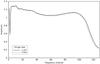 |
Fig. 3 Scan-preaveraged parallel-hand (RR) autocorrelation spectra for the two continuum calibrator scans at antenna LA with extremal values of geometric fringe rate over the course of the observing run. Fringe rates are given in units of channel width, and frequency channels 1–128 span the baseband bandwidth of 4 MHz. |
4. Results
In this section we present results obtained by applying the data reduction techniques outlined above to representative observational data, chosen here to be a single epoch from a full-polarization VLBA monitoring campaign of the circumstellar v = 1, J = 1−0 SiO maser emission in the λ = 7 mm band toward the Mira variable TX Cam, scheduled as VLBA project code BD46. The results of this synoptic imaging campaign have been published in total intensity by Diamond & Kemball (2003) and Gonidakis et al. (2010), and in linear polarization by Kemball et al. (2009). We choose epoch BD46AQ as a representative dataset for this work, as it contains polarization EVPA reversals at the circumstellar boundary and is therefore of independent scientific interest, but for no other special technical reason. The data were reduced for this epoch following the heuristics outlined in Sect. 3 and we highlight results relevant to the current data reduction method in this section.
Full details of the observing configuration for the project BD46AQ are described in the original references above; we provide only a concise synopsis here. The effective observing time was 6.5 h, allocated between the target source TX Cam and extra-galactic continuum calibrators 3C454.3, J0359+509, and J0609-157. The v = 1, J = 1−0 SiO transition was centered in a 4 MHz baseband and cross-correlated in full polarization over 128 frequency channels with a correlator accumulation interval of 4.99 s. The array comprised all ten VLBA antennas and a single antenna from the VLA. The VLBA antenna at Mauna Kea (MK) did not contribute data due to operational difficulties.
The data were sampled in one-bit quantization; digital corrections for sampling and quantization where derived using methods described above. The derived quantization corrections have low magnitude ≤ 0.5% and are stable in time, as expected for one-bit quantization. After these corrections, the antenna-based autocorrelation bandpass amplitude responses were solved for in Chebyshev polynomial form using the methods of Sect. 3.2. The bandpass frequency-frame considerations discussed in that section are illustrated in Fig. 3; this figure shows two parallel-hand continuum calibrator autocorrelation spectra produced by the VLBA correlator for a single antenna, here Los Alamos (LA), pre-averaged over time in the bandpass solver. These spectra are in a geocentric reference frame, and this figure shows the two scans that have extremal natural fringe-rate offsets between the topocentric and geocentric frequency reference frames over the course of the observation. As noted in Sect. 2, the polynomial bandpass solver accommodates the frequency shift algebraically in the Chebyshev expansion for the bandpass response function, without needing to interpolate the sampled data in frequency, and can use fewer free parameters than the total number of frequency channels Nc as a result. The matching full topocentric channel range needs to be used in the fit however, as opposed to [1..Nc] , in order to provide a maximal constraint on χ2 across the band. An expanded view of the frequency shifts in the scan pre-averaged data near the upper spectral roll-off is shown in Fig. 4; this depicts a subset of scans spanning the full range of natural fringe rate in the data for the Los Alamos antenna.
 |
Fig. 4 Scan-preaveraged parallel-hand (RR) autocorrelation spectra in the upper spectral roll-off region of the baseband for a subset of continuum calibrator scans at antenna LA spanning the range of geometric fringe-rate over the course of the observing run. Fringe rates are given in units of channel width, and frequency channels 1–128 span the baseband bandwidth of 4 MHz. |
As described in Sect. 3.2, a correction for aliasing is required if the high-SNR autocorrelation bandpass amplitude response functions are to be used to correct the cross-correlation data. The results of the aliasing correction are presented for a selection of representative antennas in Fig. 5; here shown in the RCP bandpass response functions for this antenna subset. For each antenna, a separate amplitude response is plotted for: i) the original autocorrelation bandpass; ii) a cross-correlation bandpass estimate; and; iii) the alias-corrected response. Note the low SNR of the cross-correlation bandpass response obtained from Eq. (25), for reasons described in that section.
The alias-corrected amplitude response preserves the SNR of the autocorrelation bandpass solution while correcting both the mid-band mean amplitude and upper band-edge frequency response, so that it can be used to correct cross-correlation data more accurately. This improvement in performance when correcting cross-correlation amplitudes is shown in Fig. 8. The final component of bandpass determination is the correction for the differential polarization phase response at the reference antenna, derived from the cross-polarized autocorrelation spectra as described in Sect. 3. The R-L bandpass phase response as solved for from the RL and LR autocorrelation spectra at the reference antenna LA is shown in Fig. 6. The corrected cross-polarized RL autocorrelation spectrum at LA, after correction for the R-L bandpass phase response is plotted in Fig. 7.
The data were then calibrated in amplitude using the autocorrelation polarization self-calibration algorithm described in Sect. 3.3.3. This method refines the standard template-fitting method to allow the use of a mean multi-antenna template spectrum with higher SNR, depicted here in Fig. 9 for both parallel hands. The method also provides an independent calibration of the differential polarization amplitude gain gR/L (Eq. (35)), and uses the full non-linear autocorrelation polarization data model including self-noise, as described in Eq. (8). An example of fitting this equation to the autocorrelation spectra at the reference antenna LA is shown in Fig. 10. As described earlier, the chi-square minimization in this fit is performed over all Stokes autocorrelation polarization pairs; however for clarity of presentation we show the real-valued Stokes Q spectra pre-averaged over each scan in the form of both the original data and the fitted model. Each scan is annotated by the corresponding parallactic angle. The time-variability of the Stokes Q spectra across the observation arises from both the parallactic angle terms in Eq. (8) as well as the D-term mediated corruptions from the autocorrelation spectra in other Stokes polarization pairs. As described in Sect. 3.3.3, an iterative polarization self-calibration method is used to refine both the true source model correlation spectrum and the instrumental terms, including D-terms and the differential polarization phase and group-delay offsets. In Fig. 11 we show the rapid iterative convergence of the RL source model correlation spectrum over three iterations: the initial and final model spectra are plotted here.
 |
Fig. 5 Bandpass amplitude response function solutions in RCP for a subset of representative antennas obtained from: i) autocorrelation calibrator data (dotted line) by solving Eq. (19); ii) cross-correlation calibrator data (dashed line) by solving Eq. (25); and iii) the autocorrelation bandpass solutions corrected for a fitted aliasing model (solid line), as defined by Eq. (26). |
As a test of net error in Stokes V the amplitude gain factors derived from TX Cam using the preceding spectral-line calibration sequence were scaled by an additional constant user-specified R/L amplitude gain factor and applied to the continuum calibrator J0359+509. The J0359+509 data were then self-calibrated in phase only, an independent D-term solution derived using the similarity polarization approximation (Kemball 1999), and imaged in Stokes {I,Q,U,V}. These images were produced over a range of such user-specified R/L amplitude gain factors. This particular continuum calibrator was observed most frequently during the schedule, and amongst the calibrators has the smallest angular separation from TX Cam on the sky. The integrated degree of circular polarization mc was then measured by integrating Stokes V and Stokes I over a rectangular region tightly enclosing the central emission in the calibrator image of J0359+509. The resultant plot of mc versus the additional user-specified R/L gain factor is shown in Fig. 12. The measured fractional circular polarization of the continuum calibrator for unit additional R/L amplitude gain factor provides an estimate of the error in the data reduction algorithm presented here. A linear fit produces a value mc = −0.3% at the nominal value where the user-specified R/L factor is unity.
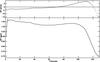 |
Fig. 6 R-L differential polarization bandpass phase response at the reference antenna LA, as measured from the cross-polarized RL and LR autocorrelation spectra. The amplitude response shown here is derived from the parallel-hand autocorrelation data. |
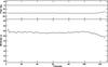 |
Fig. 7 RL autocorrelation spectrum at the reference antenna LA, corrected by the bandpass depicted in Fig. 6. |
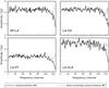 |
Fig. 8 Continuum calibrator cross-power spectral amplitudes on representative baselines to the reference antenna LA, calibrated in amplitude, group delay, and fringe rate, and averaged over the duration of the observing run; calibrated additionally either with the original autocorrelation bandpass response (solid line) or the alias-corrected bandpass response (dotted line). |
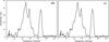 |
Fig. 9 Mean autocorrelation template spectra in RR and LL, plotted on a common y-axis of spectral flux density (Jy). Frequency channels 1–128 span the 4 MHz baseband bandwidth. |
5. Discussion
General-purpose radio-interferometric arrays are optimized in design to provide radiometric
accuracy matched primarily to the requirements of their key science goals. The a priori
amplitude calibration information provided by the VLBA, in the form of measured system
temperatures  and point source
sensitivities
and point source
sensitivities  is not the limiting final
accuracy of amplitude calibration; in many cases it can be refined to greater accuracy
(<5%) using careful subsequent amplitude self-calibration; and
the absolute flux density scale can be set to comparable accuracy using compact amplitude
calibrators of known brightness.
is not the limiting final
accuracy of amplitude calibration; in many cases it can be refined to greater accuracy
(<5%) using careful subsequent amplitude self-calibration; and
the absolute flux density scale can be set to comparable accuracy using compact amplitude
calibrators of known brightness.
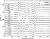 |
Fig. 10 Scan pre-averaged autocorrelation Stokes Q spectra before polarization self-calibration (dotted line) and as fitted against Eq. (8) including polarization terms (solid line). Each scan pre-average is labeled at left by parallactic angle α (in deg). |
 |
Fig. 11 Soure RL correlation total-power spectra for iteration one (S1) and three (S3) of the autocorrelation polarization self-calibration algorithm. |
 |
Fig. 12 Measured circular polarization mc of the continuum calibrator J0359+509 after application of the TX Cam spectral–line amplitude calibration and an additional user-specified R/L amplitude gain factor. The continuum calibrator circular polarization measurement for unit additional R/L gain factor provides a single measurement of the error in mc for the data reduction algorithm presented here. This intercept value is mc = −0.3%. |
Amplitude self-calibration refinement in this broader context, traditionally applied to
continuum parallel-hand data, requires imposition of an external constraint on
Stokes V however. Invariably, Stokes V ~ 0 is assumed
for individual continuum calibrator or target sources. However, as noted above, the more
selective constraint that an ensemble of continuum target sources should have mean
 (Homan & Wardle 1999) allows non-zero
mc to be measured for individual sources to higher accuracy.
For spectral-line sources, an analogous assumption of zero mean circular polarization across
frequency
(Homan & Wardle 1999) allows non-zero
mc to be measured for individual sources to higher accuracy.
For spectral-line sources, an analogous assumption of zero mean circular polarization across
frequency  could be made for an individual source, however in the latter case this must always be in
essence an ad hoc assumption. The mean net
could be made for an individual source, however in the latter case this must always be in
essence an ad hoc assumption. The mean net  for a given SiO maser source depends on a number of unknown physical properties of the
source, e.g. magnetic field orientation and the morphological distribution of maser
components across the source.
for a given SiO maser source depends on a number of unknown physical properties of the
source, e.g. magnetic field orientation and the morphological distribution of maser
components across the source.
In the current paper we have shown that it is possible to measure circular polarization in spectral-line VLBI observations at millimeter wavelengths to a far higher level of accuracy (<1%) than suggested by the absolute accuracy of the a priori amplitude calibration information (10−15%), but without the need to perform amplitude self-calibration. This is possible by relying instead on the amplitude gain information encoded in the high-SNR autocorrelation spectra, which are additionally constrained to measure a common (antenna-independent) source correlation spectrum J(ω). This principle was recognized early in the development of the template-fitting method of amplitude calibration for spectral line VLBI (Reid et al. 1980); in the current work we have shown that it is possible to enhance this approach sufficiently to extend it to accurate circular polarization measurements at millimeter observing wavelengths. This approach has the advantage of avoiding amplitude self-calibration, which is statistically less robust when solving for antenna amplitude gain factors across sparse arrays when observing sources with complex spatial structure.
In Fig. 13, we show a plot of the polarization ratio of template-fitted amplitude gains for each antenna in each of the two orthogonal receptor polarizations against the value of the RR template-fitted gain derived as part of the same calibration. The amplitude gain factors are expected to increase with increasing atmospheric airmass along the line of sight or with increasing pointing error. These two effects are also partially coupled due to the expected increase in residual pointing rms at low elevation for mechanical reasons. The structure in this figure, especially when examined for individual antennas, is consistent with differential polarization amplitude gain effects due to pointing errors in the presence of beam squint (see Eq. (3)), and suggests the template-fitting method is correcting the associated amplitude gain effects. This effect is more pronounced at 3 mm, as expected.
 |
Fig. 13 Parallel-hand template-fitted amplitude gain factors for each antenna derived from the mean template spectra (Fig. 9), plotted as differential polarization amplitude gain ratios against the RR amplitude gain derived by the same method. |
We next consider the applicability of the algorithm we have presented in this paper. It does both require sufficient SNR in the autocorrelation spectra, and adequate spectral structure in the source emission so that the source spectrum is sufficiently mathematically non-degenerate relative to continuum baseline terms of polynomial form. However, these conditions are broadly met in observations of strong maser emission in these bands.
Our implementation of autocorrelation polarization self-calibration here has allowed an assessment the impact of second-order instrumental polarization terms on the parallel-hand autocorrelation spectra, and on the resultant amplitude gain factors estimated using the revised template-fitting method. Our conclusion from the current study is that this correction is helpful if the autocorrelation data have sufficient SNR and an adequate range of parallactic angle coverage. The SNR condition typically holds at λ = 7 mm but may not be routinely applicable at λ = 3 mm, due to the significantly higher SEFD in the latter band. Given the low D-term magnitude at the VLBA, in the low-SNR case the autocorrelation polarization self-calibration step may not be of net benefit and can be omitted.
Where applicable in terms of SNR however, we find the autocorrelation polarization method to be strongly convergent, especially when deriving an initial estimate of the cross-polarized autocorrelation source model using zero mean phase averaging, as noted above. This convergence is apparent in Fig. 11.
We note that the computational cost of the algorithms described in this paper is modest, broadly comparable to regular self-calibration.
Further work would be beneficial in several key areas. An exploration is needed of optimal polynomial bases for the expansion of complex bandpass responses, as a possible alternative to the Chebyshev basis used here, and especially for the low-SNR regime at these observing wavelengths. In some low-SNR cases the Chebyshev expansion will over-fit the noise and introduce low-level quasi-sinusoidal ripple. Opimized spectral baseline removal methods for the low-SNR case would likely improve both the template-fitting and autocorrelation polarization self-calibration elements. In addition, and most importantly, the data reduction technique described here needs to be applied to a greater sample of sources in order to set both the required SNR limit more precisely and to obtain a more comprehensive measurement of the statistical performance of the algorithm as an estimator for mc and Stokes V over a greater source sample.
From the current work, we estimate the accuracy of the full algorithm presented in this paper as mc ≤ 0.5% or better at λ = 7 mm, and mc ≤ 0.5−1% or better at λ = 3 mm. We base this estimate on measurements of Stokes V in associated continuum calibrators, as shown in Fig. 12 for the test data BD46AQ considered here. These figures are also broadly consistent with sub-sampling bootstrap resampling tests on the variance of gR/L estimated using Eq. (35). We note that both these tests tend to over-estimate the error in mc as both are affected by interpolation errors from the position of the target source to the position of the continuum calibrator. These interpolation errors include differences in pointing errors and airmass along the lines of sight to the two separate sources. As noted above, further tests with larger source samples would be helpful in this regard.
The technique presented here however has significant scientific application in the study of circular polarization of astrophysical masers in these observing bands. This is especially true for SiO masers, for which accurate Stokes V measurements provide strong constraints on models of polarized maser propagation, and correspondingly of associated estimates of astrophysical magnetic fields.
6. Conclusions
The conclusions of our work are as follows:
-
1.
We have examined the sources of calibration error in spectral-line VLBI imaging observations at λ = 7 mm and λ = 3 mm sensitive to circular polarization. This analysis was performed with a specific emphasis on SiO maser observations using the VLBA.
-
2.
A algorithm is presented to provide accurate calibration of circular polarization without using amplitude self-calibration. This method is an enhancement of existing spectral-line VLBI calibration methods based on autocorrelation data, but with several innovations in bandpass estimation, autocorrelation polarization self-calibration, and the adaption of techniques for the low-SNR regime applicable at millimeter wavelengths.
-
3.
We demonstrate an example reduction at λ = 7 mm and provide an estimate of circular polarization accuracy of mc ≤ 0.5% or better at λ = 7 mm and mc ≤ 0.5−1% or better at 3 mm. These estimates are based on Stokes V imaging of associated continuum calibrators and a statistical analysis of uv-data differential polarization amplitude ratios.
The National Radio Astronomy Observatory is a facility of the National Science Foundation operated under cooperative agreement by Associated Universities, Inc.
Acknowledgments
We thank the anonymous referee for their insightful comments on this paper. This material is based upon work partially supported by the National Science Foundation under grant AST-0507473. Any opinions, findings, and conclusions or recommendations expressed in this material are those of the authors and do not necessarily reflect the views of the National Science Foundation.
References
- Attridge, J. M. 2001, ApJ, 553, L31 [NASA ADS] [CrossRef] [Google Scholar]
- Barvainis, R., McIntosh, G., & Read Predmore, C. 1987, Nature, 329, 613 [NASA ADS] [CrossRef] [Google Scholar]
- Bianchi, G., & Sorrentino, R. 2007, Electronic Filter Simulation and Design (New York, NY: McGraw Hill) [Google Scholar]
- Cawthorne, T. V., Wardle, J. F. C., Roberts, D. H., Gabuzda, D. C., & Brown, L. F. 1993, ApJ, 416, 519 [NASA ADS] [CrossRef] [Google Scholar]
- Conway, R. G., & Kronberg, P. P. 1969, MNRAS, 142, 11 [NASA ADS] [Google Scholar]
- Cotton, W. D., Geldzahler, B. J., Marcaide, J. M., et al. 1984, ApJ, 286, 503 [NASA ADS] [CrossRef] [Google Scholar]
- Deller, A. T., Tingay, S. J., Bailes, M., & West, C. 2007, PASP, 119, 318 [NASA ADS] [CrossRef] [Google Scholar]
- Diamond, P. J. 1989, in Synthesis Imaging in Radio Astronomy, ed. R. A. Perley, F. R. Schwab, & A. H. Bridle (PASP: San Francisco), 6, 379 [Google Scholar]
- Diamond, P. J., & Kemball, A. J. 2003, ApJ, 599, 1372 [NASA ADS] [CrossRef] [Google Scholar]
- Downes, D. 1989, in Evolution of Galaxies. Astronomical Observations, Proc. Astrophysics School I, Organized by the European Astrophysics Doctoral Network at Les Houches, Haute-Savoie, France, September 5–16, 1988, ed. I. Appenzeller, H. J. Habing, & P. Lena (Berlin: Springer-Verlag), 351 [Google Scholar]
- Evans, J. V., & Hagfors, T. 1968, Radar Astronomy (New York: McGraw-Hill) [Google Scholar]
- Glenn, J., Jewell, P. R., Fourre, R., & Miaja, L. 2003, ApJ, 588, 478 [NASA ADS] [CrossRef] [Google Scholar]
- Goldreich, P., Keeley, D. A., & Kwan, J. Y. 1973, ApJ, 179, 111 [NASA ADS] [CrossRef] [Google Scholar]
- Gonidakis, I., Diamond, P. J., & Kemball, A. J. 2010, MNRAS, 406, 395 [NASA ADS] [CrossRef] [Google Scholar]
- Granlund, J. 1986, O’Sullivan’s Zero-Padding, VLBA Correlator Memo, 66 (Charlottesville, VA: National Radio Astronomy Observatory) [Google Scholar]
- Habing, H. J. 1996, A&A Rev., 7, 97 [NASA ADS] [CrossRef] [Google Scholar]
- Hamaker, J. P., Bregman, J. D., & Sault, R. J. 1996, A&AS, 117, 137 [NASA ADS] [CrossRef] [EDP Sciences] [Google Scholar]
- Herpin, F., Baudry, A., Thum, C., Morris, D., & Wiesemeyer, H. 2006, A&A, 450, 667 [NASA ADS] [CrossRef] [EDP Sciences] [Google Scholar]
- Homan, D. C., & Lister, M. L. 2006, AJ, 131, 1262 [NASA ADS] [CrossRef] [Google Scholar]
- Homan, D. C., & Wardle, J. F. C. 1999, AJ, 118, 1942 [NASA ADS] [CrossRef] [Google Scholar]
- Homan, D. C., Attridge, J. M., & Wardle, J. F. C. 2001, ApJ, 556, 113 [NASA ADS] [CrossRef] [Google Scholar]
- Homan, D. C., Lister, M. L., Aller, H. D., Aller, M. F., & Wardle, J. F. C. 2009, ApJ, 696, 328 [NASA ADS] [CrossRef] [Google Scholar]
- Kemball, A. J. 1999, in Synthesis Imaging in Radio Astronomy II, A Collection of Lectures from the Sixth NRAO/NMIMT Synthesis Imaging Summer School, ed. G. B. Taylor, C. L. Carilli, & R. A. Perley, ASP Conf. Ser., San Francisco, 180, 499 [Google Scholar]
- Kemball, A. J., & Diamond, P. J. 1997, ApJ, 481, L111 [NASA ADS] [CrossRef] [Google Scholar]
- Kemball, A. J., Diamond, P. J., & Cotton, W. D. 1995, A&AS, 110, 383 [Google Scholar]
- Kemball, A. J., Diamond, P. J., & Pauliny-Toth, I. I. K. 1996, ApJ, 464, L55 [NASA ADS] [CrossRef] [Google Scholar]
- Kemball, A. J., Crutcher, R. M., & Hasan, R. 2008, Softw. Pract. Exper., 38, 493 [CrossRef] [Google Scholar]
- Kemball, A. J., Diamond, P. J., Gonidakis, I., et al. 2009, ApJ, 698, 1721 [NASA ADS] [CrossRef] [Google Scholar]
- Kogan, L. 1993a, B-factor of FX Correlator for Different Pairs of Digitizers, Two- and Four-level Quantization, VLBA Scientific Memo. No. 6 (Socorro, NM: National Radio Astronomy Observatory) [Google Scholar]
- Kogan, L. 1993b, An Investigation of the Conversion Function from the True Correlation to the Measured One if the Input Signals are Quantized Differently, Two- and Four-Level Quantization, VLBA Scientific Memo, 5 (Socorro, NM: National Radio Astronomy Observatory) [Google Scholar]
- Kogan, L. 1995, Effect of Digitizer Errors on the Cross- and Auto-Correlation Response of an FX Correlator, VLBA Scientific Memo. No. 9 (Socorro, NM: National Radio Astronomy Observatory) [Google Scholar]
- Kogan, L. 1998, Radio Sci., 33, 5, 1289 [CrossRef] [Google Scholar]
- Kutner, M. L., & Ulich, B. L. 1981, ApJ, 250, 341 [NASA ADS] [CrossRef] [Google Scholar]
- Leppänen, K. 1993, Opacity Correction for High Frequency VLBI Observations, VLBA Scientific Memo. No. 1 (Socorro, NM: National Radio Astronomy Observatory) [Google Scholar]
- Napier, P. 1995, in Proceedings of a Summer School held in Socorro, New Mexico, 23–30 June 1993, ed. J. A. Zensus, P. J. Diamond, & P. J. Napier (San Francisco, CA: ASP), ASP Conf. Ser. 82, 59 [Google Scholar]
- Nash, S. G. 1984, SIAM J Num Anal, 21, 770 [CrossRef] [Google Scholar]
- Nocedal, J. 1980, Math. Comput., 35, 773 [CrossRef] [Google Scholar]
- Liu, D. C., & Nocedal, J. 1989, Math. Prog. B, 45, 3, 503 [Google Scholar]
- Pollack, L. K., Taylor, G. B., & Zavala, R. T. 2003, ApJ, 589, 733 [NASA ADS] [CrossRef] [Google Scholar]
- Press, W. H., Teukolsky, S. A., Vetterling, W. T., & Flannery, B. P. 2007, Numerical Recipes (New York, NY: Cambridge University Press) [Google Scholar]
- Reid, M. J., Haschick, A. D., Burke, B. F., et al. 1980, ApJ, 239, 89 [NASA ADS] [CrossRef] [Google Scholar]
- Roberts, D. H., Wardle, J. F. C., & Brown, L. F. 1994, ApJ, 427, 718 [NASA ADS] [CrossRef] [PubMed] [Google Scholar]
- Romney, J. D. (Ed.) 2010, VLBA Observational Status Summary (Socorro, NM:NRAO), http://www.vlba.nrao.edu/astro/obstatus/current/ [Google Scholar]
- Sault, R. J., Hamaker, J. P., & Bregman, J. D. 1996, A&AS, 117, 149 [NASA ADS] [CrossRef] [EDP Sciences] [Google Scholar]
- Thompson, A. R. 1995, in Very Long Baseline Interferometry and the VLBA, NRAO Workshop, Proc. a Summer School held in Socorro, New Mexico, 23–30 June 1993, ed. J. A. Zensus, P. J. Diamond, & P. J. Napier (San Francisco: ASP), ASP Conf. Ser., 82, 73 [Google Scholar]
- Thompson, A. R., Moran, J. M., & Swenson, G. W. 2001, Interferometry and Synthesis in Radio Astronomy (New York, NY: Wiley) [Google Scholar]
- Troland, T. H., Heiles, C., Johnson, D. R., & Clark, F. O. 1979, ApJ, 232, 143 [NASA ADS] [CrossRef] [Google Scholar]
- Vlemmings, W. H. T., Diamond, P. J., & van Langevelde, H. J. 2002, A&A, 394, 589 [NASA ADS] [CrossRef] [EDP Sciences] [Google Scholar]
- Walker, R. C. 1999, in Synthesis Imaging in Radio Astronomy II, ed. G. B. Taylor, C. L. Carilli, & R. A. Perley (San Francisco, CA: ASP), ASP Conf. Ser., 180, 433 [Google Scholar]
- Wardle, J. F. C., Roberts, D. H., Potash, R. I., & Rogers, A. E. E. 1986, ApJ, 304, L1 [NASA ADS] [CrossRef] [Google Scholar]
- Wiesemeyer, H. 2009, A&A, 501, 647 [NASA ADS] [CrossRef] [EDP Sciences] [Google Scholar]
- Wiesemeyer, H., Thum, C., Baudry, A., & Herpin, F. 2009, A&A, 498, 801 [NASA ADS] [CrossRef] [EDP Sciences] [Google Scholar]
- Wilson, T. L., Rohlfs, K., & Hüttemeister, S. 2009, Tools of Radio Astronomy (Berlin Heidelberg: Springer-Verlag) [Google Scholar]
All Tables
All Figures
|
Fig. 1 Plot of normalized primary beam patterns in 1-d cross-section for receptor
polarizations {R,L} with a beam squint equal to 5% of the
full-width at half-maximum θb; the
x-ordinate for the beam pattern plot is in units of
θb. The ratio of the two beam
patterns is also plotted in the upper part of the diagram as a function of pointing
error ϵp, with x-ordinate
|
| In the text | |
|
Fig. 2 Flowchart depicting the overall data reduction sequence described in Sect. 3. |
| In the text | |
|
Fig. 3 Scan-preaveraged parallel-hand (RR) autocorrelation spectra for the two continuum calibrator scans at antenna LA with extremal values of geometric fringe rate over the course of the observing run. Fringe rates are given in units of channel width, and frequency channels 1–128 span the baseband bandwidth of 4 MHz. |
| In the text | |
|
Fig. 4 Scan-preaveraged parallel-hand (RR) autocorrelation spectra in the upper spectral roll-off region of the baseband for a subset of continuum calibrator scans at antenna LA spanning the range of geometric fringe-rate over the course of the observing run. Fringe rates are given in units of channel width, and frequency channels 1–128 span the baseband bandwidth of 4 MHz. |
| In the text | |
|
Fig. 5 Bandpass amplitude response function solutions in RCP for a subset of representative antennas obtained from: i) autocorrelation calibrator data (dotted line) by solving Eq. (19); ii) cross-correlation calibrator data (dashed line) by solving Eq. (25); and iii) the autocorrelation bandpass solutions corrected for a fitted aliasing model (solid line), as defined by Eq. (26). |
| In the text | |
|
Fig. 6 R-L differential polarization bandpass phase response at the reference antenna LA, as measured from the cross-polarized RL and LR autocorrelation spectra. The amplitude response shown here is derived from the parallel-hand autocorrelation data. |
| In the text | |
|
Fig. 7 RL autocorrelation spectrum at the reference antenna LA, corrected by the bandpass depicted in Fig. 6. |
| In the text | |
|
Fig. 8 Continuum calibrator cross-power spectral amplitudes on representative baselines to the reference antenna LA, calibrated in amplitude, group delay, and fringe rate, and averaged over the duration of the observing run; calibrated additionally either with the original autocorrelation bandpass response (solid line) or the alias-corrected bandpass response (dotted line). |
| In the text | |
|
Fig. 9 Mean autocorrelation template spectra in RR and LL, plotted on a common y-axis of spectral flux density (Jy). Frequency channels 1–128 span the 4 MHz baseband bandwidth. |
| In the text | |
|
Fig. 10 Scan pre-averaged autocorrelation Stokes Q spectra before polarization self-calibration (dotted line) and as fitted against Eq. (8) including polarization terms (solid line). Each scan pre-average is labeled at left by parallactic angle α (in deg). |
| In the text | |
|
Fig. 11 Soure RL correlation total-power spectra for iteration one (S1) and three (S3) of the autocorrelation polarization self-calibration algorithm. |
| In the text | |
|
Fig. 12 Measured circular polarization mc of the continuum calibrator J0359+509 after application of the TX Cam spectral–line amplitude calibration and an additional user-specified R/L amplitude gain factor. The continuum calibrator circular polarization measurement for unit additional R/L gain factor provides a single measurement of the error in mc for the data reduction algorithm presented here. This intercept value is mc = −0.3%. |
| In the text | |
|
Fig. 13 Parallel-hand template-fitted amplitude gain factors for each antenna derived from the mean template spectra (Fig. 9), plotted as differential polarization amplitude gain ratios against the RR amplitude gain derived by the same method. |
| In the text | |
Current usage metrics show cumulative count of Article Views (full-text article views including HTML views, PDF and ePub downloads, according to the available data) and Abstracts Views on Vision4Press platform.
Data correspond to usage on the plateform after 2015. The current usage metrics is available 48-96 hours after online publication and is updated daily on week days.
Initial download of the metrics may take a while.