| Issue |
A&A
Volume 533, September 2011
|
|
|---|---|---|
| Article Number | A40 | |
| Number of page(s) | 14 | |
| Section | The Sun | |
| DOI | https://doi.org/10.1051/0004-6361/201116749 | |
| Published online | 24 August 2011 | |
Dynamo action and magnetic buoyancy in convection simulations with vertical shear
1
NORDITA, Roslagstullsbacken 23,
10691
Stockholm,
Sweden
e-mail: This email address is being protected from spambots. You need JavaScript enabled to view it.
2
Department of Physics, Gustaf Hällströmin katu 2a, PO Box 64, 00014 University of Helsinki,
Finland
Received:
18
February
2011
Accepted:
11
July
2011
Abstract
Context. A hypothesis for sunspot formation is the buoyant emergence of magnetic flux tubes created by the strong radial shear at the tachocline. In this scenario, the magnetic field has to exceed a threshold value before it becomes buoyant and emerges through the whole convection zone.
Aims. We follow the evolution of a random seed magnetic field with the aim of study under what conditions it is possible to excite the dynamo instability and whether the dynamo generated magnetic field becomes buoyantly unstable and emerges to the surface as expected in the flux-tube context.
Methods. We perform numerical simulations of compressible turbulent convection that include a vertical shear layer. Like the solar tachocline, the shear is located at the interface between convective and stable layers.
Results. We find that shear and convection are able to amplify the initial magnetic field and form large-scale elongated magnetic structures. The magnetic field strength depends on several parameters such as the shear amplitude, the thickness and location of the shear layer, and the magnetic Reynolds number (Rm). Models with deeper and thicker tachoclines allow longer storage and are more favorable for generating a mean magnetic field. Models with higher Rm grow faster but saturate at slightly lower levels. Whenever the toroidal magnetic field reaches amplitudes greater a threshold value which is close to the equipartition value, it becomes buoyant and rises into the convection zone where it expands and forms mushroom shape structures. Some events of emergence, i.e. those with the largest amplitudes of the initial field, are able to reach the very uppermost layers of the domain. These episodes are able to modify the convective pattern forming either broader convection cells or convective eddies elongated in the direction of the field. However, in none of these events the field preserves its initial structure. The back-reaction of the magnetic field on the fluid is also observed in lower values of the turbulent velocity and in perturbations of approximately three per cent on the shear profile.
Conclusions. The results indicate that buoyancy is a common phenomena when the magnetic field is amplified through dynamo action in a narrow layer. It is, however, very hard for the field to rise up to the surface without losing its initial coherence.
Key words: magnetohydrodynamics (MHD) / convection / turbulence / Sun: dynamo / stars: magnetic field
© ESO, 2011
1. Introduction
Sunspots appear at the solar surface following an 11-year cycle. They reveal the presence of strong magnetic fields in the solar interior, and suggest the existence of a dynamo process governing its evolution. However, the process by which sunspots are formed is still debated. At the solar surface, sunspots are observed as bipolar patches of radial magnetic field. This intuitively suggests that they are formed by the emergence of horizontal concentrations of magnetic field lines, often called magnetic flux tubes. Since Parker’s original proposal of magnetic buoyancy (Parker 1955), buoyancy models have evolved through the thin flux tube approximation (Spruit 1981; Caligari et al. 1995; Fan & Fisher 1996), to numerical simulations of the emergence of 3D magnetic flux tubes. These have studied the rise of magnetic flux tubes either from the base of the convection zone (e.g. Fan 2001; Abbett et al. 2001; Fan 2008) or from the uppermost subsurface layers (see e.g., Cheung et al. 2008; Martínez-Sykora et al. 2008, and references therein). The buoyant rise of flux tubes from the tachocline up to the surface is currently the most widely accepted mechanism of sunspot formation. During the last three decades much work has been done in order to understand the buoyancy phenomena and to reconcile the results of flux tube models with phenomenological sunspots rules such as Joy’s law or the topological difference between the two spots in a pair. In spite of the fact that these basic observations have been qualitatively reproduced by the flux tube models, a set of complications has questioned the feasibility of this scenario. These may be summarized as follows:
Magnetic flux tubes at the base of the convection zone should have a strength of around 105 G in order to become unstable and then cross the entire convection zone up to the surface (Caligari et al. 1995). This has been considered a problem since the magnetic energy density corresponding to such a field is one to two orders of magnitude larger than the kinetic energy of the turbulent motions (the equipartition energy). Note, however, that in the presence of shear this is not any longer an upper limit for the amplitude of the magnetic field (see e.g. Käpylä & Brandenburg 2009).
Sunspots are coherent magnetic structures which means that the flux tubes should preserve their integrity while they rise through the entire convection zone. However, this region is highly turbulent and stratified, spanning more than 20 pressure scale heights, so in addition to the 105 G strength, the tubes must have a certain amount of twist in order to resist the turbulent diffusion (see e.g. Emonet & Moreno-Insertis 1998; Fan et al. 2003). The current results do not conclusively yield the amount of twist required for the tubes to rise coherently up to the surface. On one hand, 2D simulations require a larger twist in order to prevent the fragmentation of the flux tube in two tubes due to the vorticity generated by the buoyant rise (Schüssler 1979; Moreno-Insertis & Emonet 1996; Longcope et al. 1996; Emonet & Moreno-Insertis 1998; Fan et al. 1998). On the other hand, rising 3D flux tubes require less twist thanks to the tension forces due to the longitudinal curvature of the tube (Fan 2001). Three dimensional simulations in spherical coordinates require fine tuning of the initial twist for the tubes to emerge to the surface with the observed tilt (Fan 2008).
Magnetohydrodynamic simulations of convection in Cartesian coordinates have been able to produce large-scale magnetic fields through α2 (Käpylä et al. 2009b) and αΩ (Käpylä et al. 2008) dynamo action. However, the magnetic fields generated in these simulations are more homogeneously distributed in space rather than in the form of isolated magnetic structures. To date, however, no direct simulations, starting from the amplification of a seed magnetic field, have been able to spontaneously form sunspot-like magnetic structures.
Furthermore, instead of showing signs of buoyant rise and emergence of the magnetic field, the 3D dynamo simulations above have shown that the magnetic field is pumped down by convective downflows and tends to remain in the stable layer (see also Tobias et al. 1998, 2001; Ossendrijver et al. 2002). Fan et al. (2003) studied the evolution of an isolated twisted flux tube in a turbulent convection zone. They found that coherent rise is possible as far as the magnetic buoyant force overcomes the hydrodynamic force from convection, i.e., obeying the condition B0 > (HP/a)1/2Beq, where B0 is the initial magnetic field strength, HP is the pressure scale height, and a is the radius of the tube. In their case where (HP/a)1/2 ≈ 3, magnetic flux tubes with B0 ≥ 3Beq are able to rise coherently without being affected by convection. Similar results were found in a similar setup in spherical geometry (Jouve & Brun 2009). However, this does not address the issue of pumping since, firstly, a strong magnetic flux tube is imposed in the convective layer, and secondly, magnetic pumping is an effect related to the gradient of turbulence intensity (Kichatinov & Rüdiger 1992), which is not important in these simulations.
In addition to the thin flux tube approximation and simulations of rising flux tubes in stratified atmospheres, other attempts have found the formation of magnetic structures due to localized shear layers (Cline et al. 2003). They found that if the initial magnetic field is weak, its evolution is described be diffusive decay. On the other hand, if the imposed field is sufficiently large to become buoyant, then a hydrodynamic, of Kelvin-Helmholtz type, instability, together with the buoyancy instability will produce an α effect able to sustain the dynamo. Convection is not considered in this case. More recent efforts have been made in order to simulate the formation of a magnetic layer through the interaction of an imposed shear in convectively stable (Vasil & Brummell 2008) and unstable (Silvers et al. 2009a) atmospheres, with an imposed vertical magnetic field. They have found that, unlike in the cases of imposed toroidal magnetic layers, the buoyancy instability is harder to excite when the magnetic field is generated by the shear. More recently Silvers et al. (2009b), have found, with a similar setup, that the buoyancy may be favored by the presence of double-diffusive instabilities (these in turn depend on the ratio between the thermal and magnetic diffusivities, χ/η, often known as the inverse Roberts number). Later independent study of Chatterjee et al. (2011) has confirmed this result. However, in most of the current models, the presence of stratified turbulence, self-consistent generation of the magnetic field, or both, are omitted.
In view of the above mentioned issues, other mechanisms have been proposed in order to explain sunspots. These are related to instabilities due to the presence of a diffuse large-scale magnetic field in a highly stratified turbulent medium (Kleeorin & Rogachevskii 1994; Rogachevskii & Kleeorin 2007; Brandenburg et al. 2010a,b; Käpylä et al. 2011). Mean-field models using this mechanism are able to produce strong flux concentrations, but this has not yet been achieved in direct numerical simulations.
Motivated by the lack of simulations that merge in one model the several processes that so far have been simulated separately, here we present numerical simulations of compressible turbulent convection with an imposed flow with radial shear located in a sub-adiabatic layer beneath the convective region. For numerical reasons we do not include rotation in our setup, i.e. the turbulence is not helical, and an αΩ dynamo is not expected. Nevertheless, recent studies have shown that mean-field dynamo action is possible due to non-helical turbulence and shear (Brandenburg 2005a; Yousef et al. 2008a,b; Brandenburg et al. 2008). The nature of this dynamo is not yet entirely clear and may be attributed to the so called shear-current effect (Rogachevskii & Kleeorin 2003, 2004) or to the incoherent (stochastic) α-effect (Vishniac & Brandenburg 1997). According to Brandenburg et al. (2008) the latter explanation is consistent with the turbulent transport coefficients.
Based on these results, we expect the development of a mean magnetic field, i.e. dynamo action, in a system that mimics, as far as possible, the conditions of the solar interior, specifically in the lower part of the convection zone and the tachocline. As the shear is localized in a very narrow layer, we also expect the formation of a magnetic layer and the subsequent buoyant rise of magnetic field structures.
A similar setup was studied recently by Tobias et al. (2008). They reported the appearance of elongated stripes of magnetic field in the direction of the shear. However, since they used the Boussinesq approximation in their simulations, no magnetic buoyancy could occur. They also do not report the presence of a large scale dynamo.
Two important features distinguish the simulations presented here from previous studies in the context of flux tube formation and emergence. Firstly, we consider a highly stratified domain with ≈8 scale heights in pressure and ≈6 scale heights in density. Secondly, we do not impose a radial magnetic background field but allow the self-consistent development of the field from a initial random seed.
Even though this is a complicated setup where it is difficult to analyze the different processes independently, we believe that these simulations may shed some light on the current paradigm of sunspot formation. There are several important issues that we want to address with the following simulations. (1) What are the requirements for dynamo action in the present setup? This includes the dependence of the dynamo excitation on several parameters such as the amplitude of the shear, thickness and location of the shear layer, and the aspect ratio of the box. (2) What is the resulting configuration of the magnetic field? In particular, is the field predominantly in small or large scales, and is it organized in the form of a magnetic layer or isolated magnetic flux tubes? (3) Is the buoyancy instability (Parker 1955) operating on these magnetic structures? If yes, (4) how does it depend on the parameters listed above? (5) Is it possible to have magnetic structures strong enough to emerge from the shear layer to the surface without being affected by the turbulent convective motions? (6) Finally, it is important to study how these strong structures react back on the fluid motions, including the shear profile as well as the convective pattern.
Another important issue that may be addressed in this context is the mechanism that triggers the dynamo instability. With the recent developments on the test-field method, it is possibly to compute the dynamo transport coefficients and have a better understanding on the underlying mechanism.
We have organized this paper as follow: in Sect. 2 we provide the details of the numerical model, in Sect. 3 we describe our results. We summarize and conclude in Sect. 4.
2. The model
Our model setup is similar to that used by e.g. Brandenburg
et al. (1996) and Käpylä et al. (2008).
A rectangular portion of a star is modeled by a box whose dimensions are
(Lx,Ly,Lz) = (4,4,2)d,
where d is the depth of the convectively unstable layer, which is also
used as the unit of length. The box is divided into three layers, an upper cooling layer,
a convectively unstable layer, and a stable overshoot layer (see below). The following set
of equations for compressible magnetohydrodynamics is being solved:  (1)
(1) (2)
(2) (3)
(3) (4)where
D/Dt = ∂/∂t + U·∇
is the total time derivative. A is the magnetic vector
potential,
B = ∇ × A
is the magnetic field, and
J = ∇ × B/μ0
is the current density, μ0 is the magnetic permeability,
η and ν are the magnetic diffusivity and kinematic
viscosity, respectively, T is the temperature, s is the
specific entropy, K is the heat conductivity, ρ is the
density, U is the velocity, and
g = −gẑ is
the gravitational acceleration. The fluid obeys an ideal gas law
p = ρe(γ − 1), where p
and e are the pressure and internal energy, respectively, and
γ = cP/cV = 5/3
is the ratio of specific heats at constant pressure and volume, respectively. The specific
internal energy per unit mass is related to the temperature via
e = cVT. The rate of strain
tensor S is given by
(4)where
D/Dt = ∂/∂t + U·∇
is the total time derivative. A is the magnetic vector
potential,
B = ∇ × A
is the magnetic field, and
J = ∇ × B/μ0
is the current density, μ0 is the magnetic permeability,
η and ν are the magnetic diffusivity and kinematic
viscosity, respectively, T is the temperature, s is the
specific entropy, K is the heat conductivity, ρ is the
density, U is the velocity, and
g = −gẑ is
the gravitational acceleration. The fluid obeys an ideal gas law
p = ρe(γ − 1), where p
and e are the pressure and internal energy, respectively, and
γ = cP/cV = 5/3
is the ratio of specific heats at constant pressure and volume, respectively. The specific
internal energy per unit mass is related to the temperature via
e = cVT. The rate of strain
tensor S is given by  (5)where the commas
denote derivatives. The last term of Eq. (3)
relaxes the velocity U towards a target
profile
(5)where the commas
denote derivatives. The last term of Eq. (3)
relaxes the velocity U towards a target
profile  where
where  is a relaxation time scale. In a
non-shearing case this value corresponds to
≈1/2τturn, where
τturn = (urmskf)-1
gives an estimate of the convective turnover time. The target profile is chosen so that it
mimics the radial shear in the solar tachocline. More details of the shear profiles are
given in Sect. 2.3.
is a relaxation time scale. In a
non-shearing case this value corresponds to
≈1/2τturn, where
τturn = (urmskf)-1
gives an estimate of the convective turnover time. The target profile is chosen so that it
mimics the radial shear in the solar tachocline. More details of the shear profiles are
given in Sect. 2.3.
Summary of the runs.
The last term of Eq. (4) describes cooling
at the top of the domain according to
 (6)where
f(z) is a profile function equal to unity in
z > z3 and smoothly
going to to zero below, and Γ0 is a specific cooling luminosity chosen so that
the temperature in the uppermost layer relaxes toward
T4 = T(z = z4).
(6)where
f(z) is a profile function equal to unity in
z > z3 and smoothly
going to to zero below, and Γ0 is a specific cooling luminosity chosen so that
the temperature in the uppermost layer relaxes toward
T4 = T(z = z4).
The positions of the bottom of the box, bottom and top of the convectively unstable layer, and the top of the box, respectively, are given by (z1,z2,z3,z4) = (− 0.8,0,1,1.2)d. Initially the stratification is piecewise polytropic with polytropic indices (m1,m2,m3) = (6,1,1), which leads to a convectively unstable layer above a stable layer at the bottom of the domain and an isothermal cooling layer at the top.
2.1. Nondimensional units and parameters
Dimensionless quantities are obtained by setting
 (7)where
ρ0 is the initial density at z2.
The units of length, time, velocity, density, entropy, and magnetic field are
(7)where
ρ0 is the initial density at z2.
The units of length, time, velocity, density, entropy, and magnetic field are
![Mathematical equation: \begin{eqnarray} && [x] = d,\;\; [t] = \sqrt{d/g},\;\; [U]=\sqrt{dg},\;\; [\rho]=\rho_0, \nonumber \\ && [s]=c_{\rm P},\;\; [B]=\sqrt{dg\rho _0\mu_0}. \end{eqnarray}](/articles/aa/full_html/2011/09/aa16749-11/aa16749-11-eq81.png) (8)We
define the fluid and magnetic Prandtl numbers and the Rayleigh number as
(8)We
define the fluid and magnetic Prandtl numbers and the Rayleigh number as
 (9)where
χ0 = K/(ρmcP)
is the thermal diffusivity, and ρm is the density in the
middle of the unstable layer. For the magnetic diffusivity we consider a
z-dependent profile which gives an order of magnitude smaller value in
the radiative layer than in the convection zone through a smooth transition. Thus the
magnetic Prandtl number in the radiative layer is Pm = 15 and in the convection zone
Pm = 1.5.
(9)where
χ0 = K/(ρmcP)
is the thermal diffusivity, and ρm is the density in the
middle of the unstable layer. For the magnetic diffusivity we consider a
z-dependent profile which gives an order of magnitude smaller value in
the radiative layer than in the convection zone through a smooth transition. Thus the
magnetic Prandtl number in the radiative layer is Pm = 15 and in the convection zone
Pm = 1.5.
The entropy gradient, measured in the middle of the convectively unstable layer in the
initial non-convecting hydrostatic state, is given by  (10)where
∇−∇ad is the superadiabatic temperature gradient with
∇ad = 1−1/γ,
∇ = (∂lnT/∂lnp)zm,
and where
(10)where
∇−∇ad is the superadiabatic temperature gradient with
∇ad = 1−1/γ,
∇ = (∂lnT/∂lnp)zm,
and where  . The
amount of stratification is determined by the parameter
ξ0 = (γ − 1)cVT4/(gd),
which is the pressure scale height at the top of the domain normalized by the depth of the
unstable layer. We use in all cases ξ0 = 0.12, which results
in a density contrast of about 120. We define the fluid and magnetic Reynolds numbers via
. The
amount of stratification is determined by the parameter
ξ0 = (γ − 1)cVT4/(gd),
which is the pressure scale height at the top of the domain normalized by the depth of the
unstable layer. We use in all cases ξ0 = 0.12, which results
in a density contrast of about 120. We define the fluid and magnetic Reynolds numbers via
 (11)where
urms is the rms value of the velocity fluctuations and
kf = 2π/d
is assumed as a reasonable estimate for the wavenumber of the energy-carrying eddies. Note
that due to our definitions of the Reynolds numbers they are smaller than the usually
adopted ones by a factor of 2π. The amount of shear is quantified by
(11)where
urms is the rms value of the velocity fluctuations and
kf = 2π/d
is assumed as a reasonable estimate for the wavenumber of the energy-carrying eddies. Note
that due to our definitions of the Reynolds numbers they are smaller than the usually
adopted ones by a factor of 2π. The amount of shear is quantified by
 (12)where
U0 is the amplitude and ds the
half-width of the imposed shear profile (see below). The equipartition magnetic field is
defined by
(12)where
U0 is the amplitude and ds the
half-width of the imposed shear profile (see below). The equipartition magnetic field is
defined by  (13)For a better comparison
between the magnetic and kinetic energies, we evaluate Beq at
the center of the shear layer, z = zref.
(13)For a better comparison
between the magnetic and kinetic energies, we evaluate Beq at
the center of the shear layer, z = zref.
 |
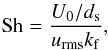
Fig. 1 Vertical profiles of mean density, pressure, temperature, specific entropy and
azimuthal velocity ( |
The simulations were performed with the Pencil Code1, which uses sixth-order explicit finite differences in space and third order accurate time stepping method.
2.2. Boundary conditions
In the horizontal (x and y) directions we use periodic
boundary conditions and at the vertical (z) boundaries we use
stress-free, impenetrable, boundary conditions for the velocity,
 (14)For the magnetic field
the vertical field condition is used on the upper boundary whereas the perfect conductor
condition is used at the lower boundary, i.e.
(14)For the magnetic field
the vertical field condition is used on the upper boundary whereas the perfect conductor
condition is used at the lower boundary, i.e.  respectively.
The upper boundary thus allows magnetic helicity flux out of the box whereas the lower
boundary does not. This is likely to be representative of the situation in a real star
where magnetic helicity can escape via the surface but does not penetrate into the core.
respectively.
The upper boundary thus allows magnetic helicity flux out of the box whereas the lower
boundary does not. This is likely to be representative of the situation in a real star
where magnetic helicity can escape via the surface but does not penetrate into the core.
Summary of runs with different aspect ratio (upper two rows) and higher resolution (lower rows).
2.3. Shear at the base of the convection zone
In order to mimic the tachocline at the base of the solar convection zone we introduce a
shear profile 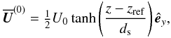 (17)where
zref is the reference position of the shear layer. Given the
uncertainties of the radial position and width of the tachocline we perform a parameter
study where zref and ds are
varied. Furthermore, it is of general interest to study how dynamo excitation depends on
varying U0 and the ratio
of U0/ds.
(17)where
zref is the reference position of the shear layer. Given the
uncertainties of the radial position and width of the tachocline we perform a parameter
study where zref and ds are
varied. Furthermore, it is of general interest to study how dynamo excitation depends on
varying U0 and the ratio
of U0/ds.
In a steady state the relaxation term that is used to impose the flow balances with the viscous term. However, if rotation is added, e.g. with Ω = Ω0(0,0,1), the Coriolis force contributes to the x-component of the velocity. In order to balance this term, e.g. with viscous term, an additional flow Ux(z) has to be generated. Such Ux(z) will then backreact on Uy and the resulting shear will be very different than that we wish to impose. Thus we refrain from adding rotation in the model in the present study.
3. Results
With the purpose of addressing the questions raised in the introduction, we perform a series of simulations with the model described above where the properties of the shear layer are varied. We first study the hydrodynamic properties of the system and the conditions for dynamo excitation. The results of this parameter study are summarized in Table 1. Then we study the topological and buoyant properties of the magnetic fields generated in some characteristic runs and compare them with models with different aspect ratio and higher resolution (see Table 2). We finalize this section with the study of the magnetic feedback on the plasma motion and the computation of the turbulent coefficients that govern the evolution of mean magnetic fields in our simulations.
3.1. Hydrodynamic instabilities
In our simulation setup, two kinds of hydrodynamical instabilities may develop, namely
the Kelvin-Helmholtz (KH) instability due to the imposed shear and stratification, and the
convective instability due to the superadiabatic stratification in the middle layer. From
hydrodynamical runs, we find that the convective instability develops early,
at t ≈ 15τturn
(≈0.8τvisc, where  ),
whereas the KH-instability starts to develop at
t ≈ 40τturn
(≈2τvisc) in runs with the strongest shear. After
a few hundred time units the velocity reaches a statistically steady state (constant
rms-velocity), and the toroidal velocity achieves the desired shear profile. A thermally
relaxed state (constant thermal energy), however, is reached only after a few thousand
time units. This time depends on the radiative conductivity (K), but also
on the imposed shear, which produces viscous heating that modifies the thermal
stratification of the system as it may be seen in the top panels of Fig. 1. The final velocity profile which includes shear,
convection, and the KH instability, does not allow the possibility of including rotation
in the model. If it is done, the system develops mean field motions in the horizontal
direction which are undesirable in the present study, as explained in Sect. 2.3.
),
whereas the KH-instability starts to develop at
t ≈ 40τturn
(≈2τvisc) in runs with the strongest shear. After
a few hundred time units the velocity reaches a statistically steady state (constant
rms-velocity), and the toroidal velocity achieves the desired shear profile. A thermally
relaxed state (constant thermal energy), however, is reached only after a few thousand
time units. This time depends on the radiative conductivity (K), but also
on the imposed shear, which produces viscous heating that modifies the thermal
stratification of the system as it may be seen in the top panels of Fig. 1. The final velocity profile which includes shear,
convection, and the KH instability, does not allow the possibility of including rotation
in the model. If it is done, the system develops mean field motions in the horizontal
direction which are undesirable in the present study, as explained in Sect. 2.3.
3.2. Dynamo excitation
 |
Fig. 2 Time evolution of the rms value of the total magnetic field normalized with the equipartition value at the center of the shear layer. Different lines/colors correspond to different runs as indicated in the legends in each panel. |
In order to study the dynamo excitation we follow the evolution of an initial random seed
magnetic field of the order of 10-5Beq. Since there
is no rotation and because the vertical component of the large-scale vorticity
 , the
average kinetic helicity and mean-field α-effect are expected to vanish
(e.g. Krause & Rädler 1980). However, it is
still possible to excite a large-scale dynamo due to non-helical turbulence and shear
(Brandenburg 2005a; Yousef et al. 2008a,b; Brandenburg et al. 2008). In this part of our study we
vary three parameters: the shear amplitude,
U0 (Runs S00−S04), the location of the shear layer in the
convectively stable region, zref (Runs D02−D04), and the
thickness of the shear region, 2ds (Runs T02−T04).
, the
average kinetic helicity and mean-field α-effect are expected to vanish
(e.g. Krause & Rädler 1980). However, it is
still possible to excite a large-scale dynamo due to non-helical turbulence and shear
(Brandenburg 2005a; Yousef et al. 2008a,b; Brandenburg et al. 2008). In this part of our study we
vary three parameters: the shear amplitude,
U0 (Runs S00−S04), the location of the shear layer in the
convectively stable region, zref (Runs D02−D04), and the
thickness of the shear region, 2ds (Runs T02−T04).
We note that no small-scale dynamo is excited in the non-shearing case. With the runs in Set S we find that the critical value of shear above which a dynamo is excited is Sh ≈ 7 (see the top panel of Fig. 2). The value of Sh is roughly three times larger than that computed with typical values of the rms-velocity and length scales in the solar tachocline2.
In Set D, we move the shear layer deeper down into the stable layer, where the turbulent
diffusivity is expected to be less, thus allowing a longer storage of the magnetic
field3. From the hydrodynamical point of view,
these simulations have a convection zone that, due to viscous heating, extends into the
initially stable layer in the saturated state as it can be seen in the vertical profile of
entropy corresponding to Run D04 (red line) in Fig. 1. The three bottom panels of the same figure (see also Table 1) show (from top to bottom) the vertical profiles of
the mean toroidal velocity ( ), the turbulent
rms-velocity and
), the turbulent
rms-velocity and  in the relaxed
state. Through out this paper we consider averages taken first over the
y direction and then the averaging over the other directions is
performed. Note that the urms-profiles have been computed
neglecting the mean flow. The curves of the turbulent velocity in the models that include
the shear layer exhibit a bump where the shear is located. This feature does not appear in
non-shearing models (see dotted line), suggesting that turbulent motions are developing in
this regions. The bump is more pronunced in models with larger Sh which indicates that
this turbulent motions are probably due to the KH instability. This difference in
urms translates into different values of the equipartition
magnetic field, Eq. (13), which hence
differs from model to model.
in the relaxed
state. Through out this paper we consider averages taken first over the
y direction and then the averaging over the other directions is
performed. Note that the urms-profiles have been computed
neglecting the mean flow. The curves of the turbulent velocity in the models that include
the shear layer exhibit a bump where the shear is located. This feature does not appear in
non-shearing models (see dotted line), suggesting that turbulent motions are developing in
this regions. The bump is more pronunced in models with larger Sh which indicates that
this turbulent motions are probably due to the KH instability. This difference in
urms translates into different values of the equipartition
magnetic field, Eq. (13), which hence
differs from model to model.
We find that the amplitude of the magnetic energy increases for deeper tachoclines. This
is an expected result since below the convection zone the magnetic diffusivity has smaller
values which allows storage of a larger magnetic flux. The vertical distribution of the
energy of the mean toroidal magnetic field ( )
peaks roughly at the center of the shear layer. The tail of this curve towards the
convection zone may hint how buoyant the magnetic field is in each model. We expect that
the larger the magnetic field (Run D04) the more magnetic flux becomes buoyant and rises
into the upper layers.
)
peaks roughly at the center of the shear layer. The tail of this curve towards the
convection zone may hint how buoyant the magnetic field is in each model. We expect that
the larger the magnetic field (Run D04) the more magnetic flux becomes buoyant and rises
into the upper layers.
The time evolution of the magnetic field of the runs in Set D are shown in the middle panel of Fig. 2. We find that the growth rate of the magnetic field, λ = dlnBrms/dt, decreases slightly as the shear layer is moved deeper. This is not very clear in Table 1 since the error of this quantity is of the same order as the difference between different runs. However, it is clear from both the figure and the table, that the volume averaged magnetic field increases with the tachocline depth.
In the third group of simulations (Runs T01−T06), we increase the width of the shear layer gradually from ds = 0.05d in Run T01 to ds = 0.20d in Run T06. This change implies lower values of the shear parameter Sh, Eq. (12), but also a larger fraction of the tachocline in the turbulent and stable layers. The results, presented in Table 1 and depicted in Figs. 1 and 2 (see legends), indicate that smaller values of the shear, Sh ≈ 3, are still able to excite the dynamo at the price of a lower growth rate. For this set of simulations we find that thicker shear layers (i.e., smaller shear values) generate a larger fraction of mean magnetic field (e.g. Runs T03 and T04). This fact is a counter-intuitive result and does not agree with previous mean-field studies on influence of the thickness of the solar tachocline (Guerrero & de Gouveia Dal Pino 2007). However, as it will be explained below, the important fact is that this configuration seems to be favorable to a longer storage of magnetic field in the stably stratified layer, with the advantage that here the effects of the shear on the thermal properties of the fluid are less important than in the previous sets of simulations. With the settings of Run T04 we find that the critical magnetic Reynolds number is between 8.1 (Run T042) and 4.1 (Run T043) as shown in Table 3. For the lower of the super-critical values of Rm (21.1 and 8.1), the magnetic field exhibits a long transient before it starts to grow. For this reason we have not ran these simulations until the field saturates. Run T043, on the contrary, Brms exhibits a clear exponential decay. We also notice that the growth rate depends on the magnetic Reynolds number.
 |
Fig. 3 Snapshots of the vertical velocity, Uz (left) and the toroidal magnetic field, By (right) in different planes of the domain, for Run T04c in the kinematic phase. The vertical slices correspond to the yz (left side of the box) and xz (front of the box) planes. The top plane corresponds to the horizontal boundary between the convective and the cooling layers at z = d and the plane shown below the box corresponds to the base of the unstable layer (z = 0). |
Summary of runs with different magnetic Reynolds number.
Based on the results above, we perform another series of simulations whose parameters and results are summarized in Table 2. Runs AR01 and AR02 correspond to Run T04 but with aspect ratios (Lx,Ly,Lz) = (8,4,2)d and (4,8,2)d, respectively. Runs D03b, and T04a to T04c have essentially the same configuration than Runs D03 and T04 with 2563 grid points resolution. The values of ν and K have been modified in order to obtain different Reynolds and Prandtl numbers.
The model with larger extent perpendicular to the direction of the shear
(x) does not show differences with respect to the reference case. On
the other hand, the model with larger extent in the direction of the shear
(y) results in a reduced growth rate and in smaller values of the
volume averaged magnetic field ( ),
the maximum amplitude of the toroidal magnetic field and of the large-scale field. The
reason for these differences is a change in the turbulent properties of the plasma for
this elongated box. We notice that the rms velocity increases for this model (AR02) which
reduces the effective value of the shear and other inductive effects. We searched for an
explanation to these differences in purely hydrodynamic, isothermal, simulations of the KH
instability (not reported here). We found that the turbulence induced by the KH
instability gives rise to mean flows which differ, in amplitude and wave number, for
different box aspect ratios. These modes may be responsible for affecting the dynamo
properties. These interesting phenomena deserve a better clarification which we postpone
to a forthcoming paper. Yousef et al. (2008a) have
obtained that both the growth rate and the scale where the maximum magnetic energy is
concentrated, converge to a value which is independent of the relevant length scale
(Lz in their case). Such convergence
analysis is computationally very expensive to be performed for our system.
),
the maximum amplitude of the toroidal magnetic field and of the large-scale field. The
reason for these differences is a change in the turbulent properties of the plasma for
this elongated box. We notice that the rms velocity increases for this model (AR02) which
reduces the effective value of the shear and other inductive effects. We searched for an
explanation to these differences in purely hydrodynamic, isothermal, simulations of the KH
instability (not reported here). We found that the turbulence induced by the KH
instability gives rise to mean flows which differ, in amplitude and wave number, for
different box aspect ratios. These modes may be responsible for affecting the dynamo
properties. These interesting phenomena deserve a better clarification which we postpone
to a forthcoming paper. Yousef et al. (2008a) have
obtained that both the growth rate and the scale where the maximum magnetic energy is
concentrated, converge to a value which is independent of the relevant length scale
(Lz in their case). Such convergence
analysis is computationally very expensive to be performed for our system.
The models with higher resolution (see Runs D03b and T04b in Table 2 and bottom panel of Fig. 2) show
a larger growth rate when compared with their corresponding low resolution cases. These
runs, however, saturate at sligthly smaller amplitudes
of .
A similar weak dependence on Rm has been reported from simulations with horizontal shear
(Käpylä et al. 2010a). We have also changed Rm by
considering a different input heat conductivity (i.e. different Pr). The results of
Runs T04a−T04c show that λ depends on Pr. There is no considerable
difference between the rms magnetic field of these runs.
3.3. Morphology of the dynamo-generated magnetic field
In the initial stages of its evolution, the magnetic field is dominated by small scales and although it is possible to distinguish the stretching effects of the shear, the structures formed are small compared with the size of the box. In Fig. 3 we present snapshots of the Run T04c in the kinematic phase.
Mean magnetic fields take longer to develop in all simulations but in the saturated state
they comprise a considerable fraction of the total field. This can be seen in the upper
panel of Fig. 4, where the ratio
 for Run S04 is
shown as a function of time. It is important to notice that mean values refer here to
averages over the y direction,
i.e.
for Run S04 is
shown as a function of time. It is important to notice that mean values refer here to
averages over the y direction,
i.e.  ,
and
,
and  .
We do not perform averaging over the x direction because the toroidal
magnetic field varies also in x (see below). The average
over x and time is performed after the mean and fluctuation values are
computed. In the same panel, the dashed line corresponds to the average value of this
ratio (
.
We do not perform averaging over the x direction because the toroidal
magnetic field varies also in x (see below). The average
over x and time is performed after the mean and fluctuation values are
computed. In the same panel, the dashed line corresponds to the average value of this
ratio ( ) in
the saturated phase of the dynamo, indicating that the mean magnetic field is roughly a
third of the total magnetic field. For the sake of clarity only a single run is shown in
this panel, but similar results are obtained for all simulations in Sets D and T.
) in
the saturated phase of the dynamo, indicating that the mean magnetic field is roughly a
third of the total magnetic field. For the sake of clarity only a single run is shown in
this panel, but similar results are obtained for all simulations in Sets D and T.
In the bottom panel of Fig. 4, the vertical profiles of the mean (solid lines) and fluctuating (dashed lines) magnetic fields for four representative runs are shown. We find that the mean magnetic field is mainly located in the shear region, whereas the turbulent field, on the other hand, is more spread out inside the convection zone. It is noteworthy that for a thick tachocline the mean field is almost comparable with the fluctuating one, covering a fraction of the stable layer where the fluctuations are weak (see solid blue line). Simulations with higher resolution (see blue lines with diamond symbols in Fig. 4) exhibit fluctuating magnetic fields with vertical distribution and magnitude almost identical to the lower resolution case. The vertical profile of the mean field is roughly the same as in the lower resolution case but of smaller magnitude.
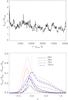 |
Fig. 4 Upper panel: ratio between the rms values of the small scale and
mean magnetic fields, brms
and |

The structure of the magnetic field depends strongly on the structure of convection. In Fig. 5 we show snapshots of vertical velocity (Uz) and azimuthal magnetic field (By) for arbitrary times in the saturated state for Runs S04, D04, and T04 (from top to bottom, respectively). From the right panels of this figure, it is possible to distinguish that at the base of the convection zone, the toroidal field organizes in elongated structures of both polarities which span all across the azimuthal direction if the penetrative (jet-like) downflows of the overshooting are less intense. These stripes coexist with more random magnetic fields in regions located where the downflows are able to reach the stable layer. The size of the magnetic structures is at least equal or larger than the scale of the convective eddies. This is more evident for the streamwise direction where the field occupies the full extent of the domain. The strong toroidal fields are mainly confined in the shear region. This can be seen in the right panels of Fig. 5 and also in the bottom panel of Fig. 1, where it is clear that the curve corresponding to Run T04 (blue line) has a broader profile than the one corresponding to Run S04 (black line). The presence of the KH instability is evident in the yz plane where wave-like structures are observed. If the tachocline is thicker, the effects of the KH-instability are weaker. Another advantage of thicker shear layers is that they do not affect the thermodynamical state of the fluid as strongly as in Sets S and T. The disadvantage is that they produce broad and more diffuse magnetic fields which do not well agree with the flux tube scenario. This is discussed in more detail in the next section.
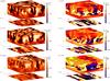 |
Fig. 5 Same as Fig. 3 but for Runs S04, D04 and T04 (from top to bottom) in the saturated phase. Movies corresponding to some of these runs may be found at: www.nordita.org/ ~guerrero. |
Although the resulting magnetic structures are buoyant (see the next section), we must clarify here that the α effect that sustains the magnetic field against diffusion here, in spite of Cline et al. (2003) does not depend, at least at the kinematic phase, on the buoyancy instability. It may result from the combination between the KH and convective instabilities. Our results are in contradiction with those of Tobias et al. (2008) who used a similar setup in the Boussinesq approximation. We believe that the lack of a large-scale dynamo in their simulations may be either due to the less step shear profile that they used or to the smaller value of the shear parameter. However, a visual inspection of their Fig. 11 suggests a large-scale dynamo with its mean field aligned in the y direction.
3.4. Buoyancy
According to linear theory (Spruit & van
Ballegooijen 1982), thin magnetic flux tubes become buoyantly unstable when the
condition
βδ > −1/γ
is fulfilled. Here
β = 2μ0p/B2
is the plasma beta, δ = ∇−∇ad is the superadiabaticity, see
Eq. (10), and γ is the
ratio of specific heats. This condition is satisfied everywhere in the convection zone
where δ > 0. From this relation it follows that
below the convection zone, where δ < 0, thin
magnetic flux tubes require a field strength beyond a threshold value to become unstable.
For a magnetic layer, the necessary and sufficient condition for the development of
two-dimensional interchange modes, in which we are interested here, is given by Newcomb (1961):  (18)We find that for the
cases with the thinnest shear layer, the instability region is above the center of the
shear layer where the toroidal magnetic field reaches its maximum value (see Fig. 6). This implies that a large fraction of the magnetic
field there becomes buoyantly unstable very quickly. For the cases with a thick shear
layer (Set T), the magnetic field is unstable only within the convection zone. The
magnetic field distribution of the Run T04 in Fig. 4
(blue line), indicates that a large fraction of the magnetic field is buoyantly stable.
This configuration may explain why in these cases larger mean magnetic fields develop with
smaller shear parameters than in Sets S and D.
(18)We find that for the
cases with the thinnest shear layer, the instability region is above the center of the
shear layer where the toroidal magnetic field reaches its maximum value (see Fig. 6). This implies that a large fraction of the magnetic
field there becomes buoyantly unstable very quickly. For the cases with a thick shear
layer (Set T), the magnetic field is unstable only within the convection zone. The
magnetic field distribution of the Run T04 in Fig. 4
(blue line), indicates that a large fraction of the magnetic field is buoyantly stable.
This configuration may explain why in these cases larger mean magnetic fields develop with
smaller shear parameters than in Sets S and D.
Note, however, that this conclusion is based on averaged quantities. The evolution of local magnetic structures is rather complex and possibly also affected by the KH instability. The shear parameter in Run T04 is smaller compared to the Runs S04 and D04, so it is expected to have a less efficient KH instability and this should allow a longer stay of the magnetic field in the stable layer. This is hard to demonstrate since it is difficult to disentangle the effects of the different instabilities (convection, KH, and buoyancy) in the simulations. Nevertheless, it seems that the longer the magnetic field stays in the stable region the greater the final mean magnetic field strength. Then, according to Fan (2001), the number of scale heights the magnetic flux concentrations may rise and its final structure depend only on how strong the field is in comparison to the turbulent convective motions.
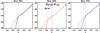 |
Fig. 6 Buoyancy instability condition, Eq. (18), evaluated for Runs S04, D04 and T04. Continuous (dashed) lines correspond to the left (right) hand side of the equation, respectively. Dotted and dot-dashed lines correspond to the interfaces between convectively stable and unstable layers, and to the center of the tachocline in each simulation, respectively. |
 |
Fig. 7 Vertical velocity (left panels) and magnetic field lines (right panels) for emergence events in Runs AR01 (top) and T04c (bottom). The colors of the magnetic field correspond to the values of By/Beq. |
In the simulations it is observed that when the magnetic field rises it expands as a consequence of decreasing density. The morphology of the magnetic fields in the xz plane (see right panels of Fig. 5) is reminiscent of the mushroom-shape that has been obtained in several 2D (Schüssler 1979; Moreno-Insertis & Emonet 1996; Longcope et al. 1996; Fan et al. 1998; Emonet & Moreno-Insertis 1998) and 3D (Fan 2001; Fan et al. 2003; Fan 2008; Jouve & Brun 2009) simulations of flux tube emergence. Such an expansion may result in the splitting and braking of the tube. We do not impose any twist on the tubes by hand since the dynamo generates the magnetic field self-consistently and the possibilities span from events that do not rise at all to events where buoyant magnetic fields rise up to the very surface. In the horizontal yz plane we observe that the magnetic field lines remain horizontal in the stable layer where they form. When the magnetic field rises, the field lines bend in the convection zone, with their rising part in the middle of upward flows and other parts withheld to the downward flows.
In Tables 1 and 2 we list the maximum values of By in the simulations. In most of the cases we find max(By) ≈ 5Beq, and only in the models with a thicker (Runs T04 and AR01) or a deeper shear layer (Run D04), max(By) can be somewhat greater than 6Beq. Fan et al. (2003) argue that if B0 > (HP/a)1/2Beq, B0 being the field strength in the shear layer and HP the local pressure scale height, a buoyant flux-tube of radius a may rise without experiencing the convective drag force. Here, although the shape of the magnetic field is not a tube, we compute the same condition using a = ds. We obtain values of B0 going from 3.4Beq in Run D04 to 2.2Beq in Run T04 (2.3Beq in corresponding higher resolution runs). This indicates that the dynamo-generated magnetic field is supposedly insufficient to reach the surface without being modified by the convection. There are, however, a few cases in Runs D04, T04 and AR01, where the strongest magnetic fields are yet able to reach the surface. When this occurs the magnetic field reacts back on the flow and modifies the convective pattern. Broad convection cells elongated in the y direction are formed. In the two upper panels of Fig. 7 we present one of these events for Run AR01. In the upper layers, the field lines show a turbulent pattern except in the center and the right edge of the box where the field lines at the surface cross the entire domain in the y direction. In the higher resolution cases, we do not observe events where the field lines, in the uppermost layers, remain horizontal accross the whole toroidal direction. Nevertheless, the expanding magnetic field may reach the surface forming broad convection cells (at least two times larger than the regular cells). One of these cases, corresponding to Run T04c is shown in the bottom panels of Fig. 7. In this event two stripes of magnetic field of opposite polarity are reaching the surface simultaneously, the magnetic field lines of these ropes reconnect forming a large scale loop oriented in the x-direction.
In order to compute the rise speed of the magnetic field in these cases we have used the horizontal averages of By and constructed the time-depth “butterfly” diagram shown in Fig. 8. The toroidal field is amplified in the shear layer, below z = 0 (see dotted line). When it becomes buoyant it travels through the convection zone. The tilt observed in the contours of By may give a rough estimate of the vertical velocity. In the same figure we have drawn correspondingly inclined white dashed lines to guide the eye. For the emergence events in Run D04 (AR01), the estimated rise speed is ub ≈ 0.034(dg)1/2 (≈0.030(dg)1/2). These values are small in comparison to the urms values of the models (see Tables 1 and 2) which does not agree with the rise of a flux tube in a stratified atmosphere. For instance, Fan et al. (2003) obtain a final rise velocity ≈5 times larger than the rms-velocity. We should point out that in the simulations here, the strong shear increases urms by a factor of two or even more. If we compare the rise velocity of the magnetic field with the rms-velocity of a non-shearing case (Run S00), we find that ub is slightly larger. Magnetic pumping effects, which are evaluated below, may also play a role in braking the rise of magnetic structures and in determining its final velocity.
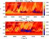 |
Fig. 8 Butterfly diagram in the depth-time plane for the horizontally averaged toroidal magnetic field, By for Runs D04 and AR01. The dotted lines corresponds to the top (z = d) and base (z = 0) of the convection zone. The tilted dashed lines show approximate trajectories of buoyant magnetic fields. A rough estimate of rise speed is computed from these lines as indicated. The event at turmskf = 9020 in the bottom panel is also shown in the top panels of Fig. 7. |
The results mentioned above do not fully agree with those found by Vasil & Brummell (2008), where a toroidal magnetic layer is generated from a purely vertical field through an imposed radial shear layer. Although their stratification is weaker than in our case, the buoyancy instability is hard to excite in their simulations and the buoyant rise events are slowed down rather quickly. The lack of a dynamo mechanism in their setup, able to sustain the magnetic field, is maybe the reason of its rapid diffusion.
3.5. Back reaction
Temporal analysis of helioseismic data has revealed that the solar angular velocity varies by around 5 per cent with respect to its mean value. The fluctuation pattern, like the sunspots, follows an 11-year cycle, which suggests that it corresponds to the back reaction of the magnetic field on the plasma motion (e.g. Basu & Antia 2003; Howe et al. 2009). It is also known that the amplitude of the meridional circulation varies with the amplitude of the magnetic field, being smaller when the cycle reaches its maximum (see e.g. Basu & Antia 2003). Apart from large scale effects, the magnetic field may also affect the local state of the plasma. This is possibly the case in the downflows found by Hindman et al. (2009); Zhao et al. (2010) nearby the bipolar active regions.
In the simulations presented here, where the dynamo presumably is different from that of the Sun, and due to the numerical setup, there are neither periodic oscillations of the magnetic field nor a large-scale circulation. We are able, however, to distinguish the differences between the plasma state in the kinematic and the saturated stages. We also follow the deviations of the averaged flow occurring during peaks of the magnetic field amplitude.
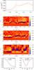 |
Fig. 9 Top: time averaged vertical profile of
urms in the kinematic (dotted line) and saturated
(solid line) stages for the Runs T04b. The dashed line shows the deviation from the
average at a one of the peaks in the magnetic field amplitude. The three
middle panels are butterfly diagrams of the angular velocity deviation,
|

We find that the turbulent rms-velocity, as well as the imposed large-scale shear flow, are affected by the magnetic field. In the top panel of Fig. 9 we show the vertical profile of the horizontal and time averaged urms in the kinematic (dotted line) and saturated (solid line) regimes of the dynamo. A decrease in the amplitude is observed, especially in the region where the magnetic field is more concentrated (dashed line). The volume averaged urms also changes accordingly by ~5 percent, as indicated in Table 2. The dashed line in the top panel of Fig. 9 shows that it further decreases in the shear region.
In the middle panels of Fig. 9, butterfly diagrams
of the toroidal velocity fluctuations,  , in the
z-time plane are shown for the Runs AR01 and T04b, respectively. The
dashed white line indicates the center of the shear layer. Positive values of this
quantity below (above) the dashed line indicate faster (slower) toroidal velocities with
respect to its mean value. Accordingly, negative values below (above) the dashed line
indicate deficiency (excess) of the local y flow. The continuous white
line corresponds to the time evolution of Brms (for clarity
normalized to its maximum value). We show this in order to demonstrate that the changes
in Uy depend on the amplitude of the
magnetic field. The overall result of the contour plots is that during the maximum of the
magnetic field the shear is slightly stronger. In these diagrams, as well as in all of the
simulations listed in Tables 1 and 2 (except Run T04τ), the deviation
from the averaged value of Uy is found to be
~3 per cent.
, in the
z-time plane are shown for the Runs AR01 and T04b, respectively. The
dashed white line indicates the center of the shear layer. Positive values of this
quantity below (above) the dashed line indicate faster (slower) toroidal velocities with
respect to its mean value. Accordingly, negative values below (above) the dashed line
indicate deficiency (excess) of the local y flow. The continuous white
line corresponds to the time evolution of Brms (for clarity
normalized to its maximum value). We show this in order to demonstrate that the changes
in Uy depend on the amplitude of the
magnetic field. The overall result of the contour plots is that during the maximum of the
magnetic field the shear is slightly stronger. In these diagrams, as well as in all of the
simulations listed in Tables 1 and 2 (except Run T04τ), the deviation
from the averaged value of Uy is found to be
~3 per cent.
The deviation of the mean shear profile depends on the forcing time
scale τf in Eq. (3). In Run T04τ, we consider the same settings as in Run T04,
but varying τf
from 2(d/g)1/2
to 10(d/g)1/2
(i.e., ≈1 to ≈5 turnover times, respectively). The results show fluctuations of
≈10 per cent of the shear velocity, and spread out to a wider fraction of the domain now
(see bottom contour plot of Fig. 9). The change in
the velocities is more clearly observed in the bottom panels of Fig. 9 where is compared
with Uy at a time when the magnetic field
peaks
(turmskf = 4700
in Run T04τ, see the dot-dashed line in the corresponding
butterfly diagram). While the profiles of the velocities are slightly different, the
instantaneous shear is clearly larger than the time-averaged one. Since magnetic buoyancy
is present also at the time of the maximum, the toroidal velocity in the middle of the
convection zone is also affected by the rising flux. This change is not so strong as the
one in the shear layer but is also a general characteristic of the simulations. Although
this is a counterintuitive result, we have verified the same effect in all the simulations
during maxima of the magnetic field strength. Disentangling the contribution of the
Lorentz force that leads to this change in the y velocity is not simple.
We conjecture that the positive contribution to the shear depends mostly on the
term BxJz
which dominates the y-component of the Lorentz force.
Similar results have been found in global numerical simulations of oscillating dynamos by Brown et al. (2011). They found torsional fluctuations in the surface angular velocity at higher latitudes (see their Fig. 11). These oscillations seem to follow the poleward migration of strong toroidal magnetic field (see the bottom panel of their Fig. 1). Correspondingly, surface fluctuations of the solar angular velocity exhibit an equatorial branch which seems to follow the contours of the strongest magnetic field. The results of the simulations presented here and those of Brown et al. (2011) are suggestive of the magnetic nature of this branch in the solar torsional oscillation pattern. Besides, a highly super-equipartition magnetic field stored at the tachocline should produce a significant change in the radial shear there. Such changes, if present, should possibly be detectable by helioseismology in forthcoming years.
3.6. Turbulent transport coefficients
In order to study the underlying mechanism of the mean-field dynamo in our simulations, we compute the turbulent transport coefficients from a representative simulation (Run T04). In order to do this, we use the test-field method, introduced in the geodynamo context by Schrinner et al. (2005, 2007) and currently available in the Pencil Code (e.g. Brandenburg 2005b; Brandenburg et al. 2008).
In mean-field theory, the electromotive force  governs the evolution of the large-scale magnetic field (Krause & Rädler 1980). We assume that there is scale separation between
the mean field and the fluctuating flow. Considering large-scale fields that depend only
on z, the electromotive force may be written in terms of the
large-scale magnetic field:
governs the evolution of the large-scale magnetic field (Krause & Rädler 1980). We assume that there is scale separation between
the mean field and the fluctuating flow. Considering large-scale fields that depend only
on z, the electromotive force may be written in terms of the
large-scale magnetic field: 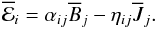 (19)Four independent test
fields are needed in order to compute the 4+4 components
of αij
and ηij (see a detailed description of
the method in Brandenburg et al. 2008). Even though
we are aware of the possible dependency of the turbulent coefficient on the scale of the
mean-field (see e.g. Chatterjee et al. 2011), we
restrict ourselves for simplicity here to linear test fields only. The novel feature of
the test-field method is that the test fields do not act back on the flow and that the
turbulent diffusivity can also be computed, thus avoiding many of the problems that plague
other methods (cf. Käpylä et al. 2010b).
(19)Four independent test
fields are needed in order to compute the 4+4 components
of αij
and ηij (see a detailed description of
the method in Brandenburg et al. 2008). Even though
we are aware of the possible dependency of the turbulent coefficient on the scale of the
mean-field (see e.g. Chatterjee et al. 2011), we
restrict ourselves for simplicity here to linear test fields only. The novel feature of
the test-field method is that the test fields do not act back on the flow and that the
turbulent diffusivity can also be computed, thus avoiding many of the problems that plague
other methods (cf. Käpylä et al. 2010b).
We discuss our results in terms of the following quantities: 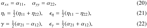 which
represent the inductive (α), diffusive (ηt),
and pumping (γ) effects of turbulence, respectively. Furthermore,
ϵη describes the anisotropy of the
turbulent diffusion, and ϵγ is the symmetric
part of the off-diagonal components of α. The latter can be related to
field-direction dependent pumping (cf. Ossendrijver et al.
2002). In Fig. 10 we show the vertical
profiles of the kinetic helicity,
which
represent the inductive (α), diffusive (ηt),
and pumping (γ) effects of turbulence, respectively. Furthermore,
ϵη describes the anisotropy of the
turbulent diffusion, and ϵγ is the symmetric
part of the off-diagonal components of α. The latter can be related to
field-direction dependent pumping (cf. Ossendrijver et al.
2002). In Fig. 10 we show the vertical
profiles of the kinetic helicity,  ,
where
ω = ∇ × u,
is the vorticity, and the turbulent transport coefficients of Eqs. (20)−(22), normalized with the first order smoothing approximation (FOSA)
quantities:
,
where
ω = ∇ × u,
is the vorticity, and the turbulent transport coefficients of Eqs. (20)−(22), normalized with the first order smoothing approximation (FOSA)
quantities: 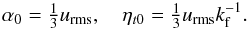 (23)For computing the
coefficients in Fig. 10 we use Run T04 in the purely
hydrodynamic state. The magnetic Reynolds number in the test field run is Rm ≈16. This
value is above the critical Rm for dynamo excitation. Previous studies have shown that the
turbulent transport coefficients for convection are independent of the magnetic Reynolds
number provided that Rm is sufficiently larger than unity (Käpylä et al. 2009a). Thus the results of this run can be considered
representative of the present setup.
(23)For computing the
coefficients in Fig. 10 we use Run T04 in the purely
hydrodynamic state. The magnetic Reynolds number in the test field run is Rm ≈16. This
value is above the critical Rm for dynamo excitation. Previous studies have shown that the
turbulent transport coefficients for convection are independent of the magnetic Reynolds
number provided that Rm is sufficiently larger than unity (Käpylä et al. 2009a). Thus the results of this run can be considered
representative of the present setup.
We find that a certain amount of helicity is generated in the system, but that it is still statistically consistent with zero. The coefficient αxx shows large fluctuations around zero. This component of α contributes to amplifying the generation of By out of Bx, but its contribution is likely to be negligible when compared with that of the shear in the present models.
The component αyy shows a zero mean value, but its variance has a large amplitude, especially in the middle of the convection zone. According to Vishniac & Brandenburg (1997), such an incoherent α effect, being zero in average but having finite variance, may generate enough inductive effects to sustain the dynamo. Hence, this effect may be is the mechanism sustaining the dynamo here.
The shear-current effect, due to the mean shear flow interacting with turbulence, may also result in the generation of a mean field (Rogachevskii & Kleeorin 2003, 2004). The existence of this effect has been studied with models of forced turbulence and latitudinal shear by (Brandenburg et al. 2008; Mitra et al. 2009), but no conclusive evidence has been found. Similar results have also been found from convection with horizontal shear (Käpylä et al. 2009a). In the case with vertical shear presented here, the relevant coefficient for this effect is not captured by the current version of the test-field method with only z-dependent test fields. Thus, we leave the study of the shear-current effect in turbulent convection with vertical shear for a forthcoming work.
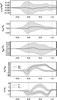 |
Fig. 10 Normalized profiles of the kinetic helicity, and the turbulent transport coefficients αxx, αyy, ηt, ϵη, γ and ϵγ (from top to bottom) computed with the test-field method. |
The turbulent diffusivity, ηt, is roughly six times larger than the FOSA estimate. This result agrees with previously computed turbulent diffusivity values for convection (Käpylä et al. 2009a). The vertical profile of ηt differs somewhat from these results, indicating the effect of the radial shear on the turbulent diffusion. Another interesting point is that ϵη is not close to zero, as in Käpylä et al. (2009a). This is likely explainable by the stronger shear used here. It is also an indication of the tensorial character of ηt and suggests that the distinct components of the magnetic field may diffuse differently.
Finally, the vertical profile of the turbulent pumping (γ) in Fig. 10 shows that there is downwards transport of the mean magnetic field almost everywhere in the convection zone and upward transport only close to the top. The pumping velocity is comparable with urms but it is not sufficient to retain the magnetic field within the stable layer, which indicates that buoyancy is a more efficient mechanism than magnetic pumping in transporting magnetic fields. The downward pumping is often attributed to the diamagnetic effect. Note, however, that the amplitude of this effect depends on the gradient of the level of turbulence, γdia = −∇ηt/2 (Kichatinov & Rüdiger 1992), which is not very large in the current simulations. However, other effects, such as non-locality can affect the pumping velocity (Käpylä et al. 2009a).
4. Conclusions
We perform numerical simulations of turbulent convection with a thin vertical shear layer with the aim of modeling some of the relevant physics of the solar convection zone and the tachocline self-consistenly. Our model includes strong shear at the base of the convection zone and magnetic buoyancy. However, our model omits the overall rotation of the star which is very likely to be important in driving the dynamo in the Sun. The shear layer is located below the interface between a convectively stable and unstable layers. We consider the velocity gradient, the position in depth and the thickness of this layer as free parameters of the model and concentrated on two phenomena relevant for the solar cycle: dynamo process and magnetic buoyancy.
We find that it is possible to excite a large scale dynamo by the combined action of turbulent convection and a localized radial shear. The efficiency of the dynamo (i.e., its growth rate), and the maximum amplitude of the magnetic field depend on the shear amplitude, the thickness of the shear layer, the aspect ratio and the magnetic Reynolds number of the system (see Fig. 2 and Tables 1 and 2).
The magnetic field is organized in elongated structures in the direction of the shear at the base, or below, of the convection zone. The large-scale magnetic field can have either polarity and its strength may reach up to 40 percent of the total field (solid lines in Fig. 4). It coexists with a turbulent magnetic field which is distributed all across the convection zone. In the stable layer the fluctuating magnetic field exists in the regions of strong downflows. For fixed depth and thickness (Set S) a larger growth rate and higher saturated Brms is obtained for a larger shear parameter. A critical value of Sh ≈ 7 is required to excite the dynamo.
If the tachocline is located deeper (simulations in set D), the magnetic field develops mainly in the convectively stable (but still to some extent turbulent) layer which allows a longer field storage. In these cases the dynamo grows faster and with a larger fraction of mean magnetic field. This configuration, however, is not optimal since with the numerical resolution used here the thermodynamical state of the fluid is affected by viscous heating in the shear region. If the depth of the shear layer remains constant but the thickness increases (Set T), the magnetic field grows more slowly but it contains a larger fraction of mean magnetic field. This may be a consequence of the smoother shear profile which renders the magnetic field buoyantly unstable only in the superadiabatic part of the domain (see right panel of Fig. 6). A lower critical shear number is found to be able to excite the dynamo instability in these cases (Sh ≈ 3).
Larger magnetic Reynolds numbers are achieved in two ways, firstly by doubling the resolution and secondly by changing the heat conductivity (i.e., changing Pr). On one side, for a fixed Pr and larger Rm, the dynamo exhibits a much faster growth. On the other hand, for a fixed resolution and different heat flux, the growth rate changes proportionally to Pr. In these higher resolution runs the final value of Brms is slightly below that in the corresponding cases with lower resolution. This may correspond to the dependence of the saturation value of the magnetic field on the magnetic Reynolds number or may also be the result of insufficient statistics.
Since the system is not rotating, there is no kinetic helicity and hence no α-effect. The test-field analysis suggests that the probable mechanism responsible for the amplification of the magnetic field could be the incoherent α-shear dynamo. However, other possibilities like the shear-current effect can not be ruled out for the time being.
Magnetic buoyancy is observed in all of the simulations. Based on horizontal averages we analyze the instability condition for 2D interchange modes (Eq. (18) and Fig. 6). We find that in models with a deeper tachocline the buoyancy instability develops even in the stable layer whereas in models with thicker shear layers the magnetic field is unstable in the convection zone only. This, however, does not mean that there are no emergence events. As far as the toroidal magnetic field is strong enough it rises through the convection zone forming mushroom-shaped structures.
When the buoyant magnetic field is weak it is strongly modified by local convective flows (see Fig. 5). On the other hand, magnetic fields of strong amplitude formed in the shear layer are able to rise up to the surface and modify the convective pattern (Fig. 7). They may form either large convection cells or convective rolls that occupy the full y-extent. The clearest events are observed when the magnetic field in the shear layer exceeds the equipartition field by a factor ≥ 6. Such strong magnetic fields have been observed only in simulations with 1283 grid points resolution. The rise velocity of the buoyant field in the bulk of the convection zone, estimated from depth-time “butterfly” diagrams, has been found to be ≈0.6urms. From the test-field method results, the maximal downward pumping velocity of magnetic field is found to be γ ≈ 0.4urms. This indicates that buoyancy is indeed efficient in transporting magnetic flux from the base of the convection zone. However, the magnetic field structures expand very quickly during the rise and magnetic structures observed close to the upper boundary are no longer so well organized.
Besides the emergence of the magnetic field that affects the flow pattern locally, other changes are observed due to the back-reaction of the magnetic field on the plasma. In the saturated phase, the rms-velocity changes from its kinematic value to a lower amplitude when the magnetic field is strong. In addition, during the peaks and valleys of the field amplitude, the imposed shear profile presents systematic variations with respect to its averaged profile. For most of the models this change is around three percent of the shear velocity and is reminiscent of the fluctuations observed in the solar rotation profile or “torsional oscillations”. The variation signal is mainly observed in the places where B is strong, with much weaker changes within the convection zone. These results encourage the study of the torsional oscillations in detail through direct numerical simulations.
We have considered ΔΩ = 33 nHz, rtac = 0.7 R⊙, dtac = 0.05 R⊙ (e.g. Christensen-Dalsgaard & Thompson 2007, and references therein), urms = 104 cm s-1, and kf = 2π/l, with l = 1010 cm (see Table 1 of Brandenburg & Subramanian 2005), which result in Shtac ≈ 2.
Note that Run S04 is the same as Runs D01 and T01.
Acknowledgments
We are thankful to the referee and Matthias Rheinhardt for their valuable comments on this work. The authors acknowledge the hospitality of NORDITA. This work is supported by the European Research Council under the AstroDyn research project 227952. The computations were performed under the HPC-EUROPA2 project (project number: 228398) with the support of the European Commission – Capacities Area – Research Infrastructures. Field line tracing figures were produced using VAPOR. P.J.K. acknowledges the financial support from the Academy of Finland grant Nos. 121431, 136189, and 140970.
References
- Abbett, W. P., Fisher, G. H., & Fan, Y. 2001, ApJ, 546, 1194 [NASA ADS] [CrossRef] [Google Scholar]
- Basu, S., & Antia, H. M. 2003, ApJ, 585, 553 [NASA ADS] [CrossRef] [Google Scholar]
- Brandenburg, A. 2005a, ApJ, 625, 539 [Google Scholar]
- Brandenburg, A. 2005b, Astron. Nachr., 326, 787 [NASA ADS] [CrossRef] [Google Scholar]
- Brandenburg, A., & Subramanian, K. 2005, Phys. Rep., 417, 1 [NASA ADS] [CrossRef] [Google Scholar]
- Brandenburg, A., Jennings, R. L., Nordlund, Å., et al. 1996, J. Fluid Mech., 306, 325 [NASA ADS] [CrossRef] [MathSciNet] [Google Scholar]
- Brandenburg, A., Rädler, K., Rheinhardt, M., & Käpylä, P. J. 2008, ApJ, 676, 740 [NASA ADS] [CrossRef] [Google Scholar]
- Brandenburg, A., Kemel, K., Kleeorin, N., & Rogachevskii, I. 2010a [arXiv:1005.5700] [Google Scholar]
- Brandenburg, A., Kleeorin, N., & Rogachevskii, I. 2010b, Astron. Nachr., 331, 5 [NASA ADS] [CrossRef] [Google Scholar]
- Brown, B. P., Miesch, M. S., Browning, M. K., Brun, A. S., & Toomre, J. 2011, ApJ, 731, 69 [NASA ADS] [CrossRef] [Google Scholar]
- Caligari, P., Moreno-Insertis, F., & Schussler, M. 1995, ApJ, 441, 886 [NASA ADS] [CrossRef] [Google Scholar]
- Chatterjee, P., Mitra, D., Rheinhardt, M., & Brandenburg, A. 2011, A&A, accepted [arXiv:1011.1218] [Google Scholar]
- Cheung, M. C. M., Schüssler, M., Tarbell, T. D., & Title, A. M. 2008, ApJ, 687, 1373 [NASA ADS] [CrossRef] [Google Scholar]
- Christensen-Dalsgaard, J., & Thompson, M. J. 2007, in The Solar Tachocline, ed. D. W. Hughes, R. Rosner, & N. O. Weiss, 53 [Google Scholar]
- Cline, K. S., Brummell, N. H., & Cattaneo, F. 2003, ApJ, 599, 1449 [NASA ADS] [CrossRef] [Google Scholar]
- Emonet, T., & Moreno-Insertis, F. 1998, ApJ, 492, 804 [NASA ADS] [CrossRef] [Google Scholar]
- Fan, Y. 2001, ApJ, 546, 509 [NASA ADS] [CrossRef] [Google Scholar]
- Fan, Y. 2008, ApJ, 676, 680 [NASA ADS] [CrossRef] [Google Scholar]
- Fan, Y., & Fisher, G. H. 1996, Sol. Phys., 166, 17 [NASA ADS] [CrossRef] [Google Scholar]
- Fan, Y., Zweibel, E. G., & Lantz, S. R. 1998, ApJ, 493, 480 [NASA ADS] [CrossRef] [Google Scholar]
- Fan, Y., Abbett, W. P., & Fisher, G. H. 2003, ApJ, 582, 1206 [NASA ADS] [CrossRef] [Google Scholar]
- Guerrero, G., & de Gouveia Dal Pino, E. M. 2007, A&A, 464, 341 [NASA ADS] [CrossRef] [EDP Sciences] [Google Scholar]
- Hindman, B. W., Haber, D. A., & Toomre, J. 2009, ApJ, 698, 1749 [NASA ADS] [CrossRef] [Google Scholar]
- Howe, R., Christensen-Dalsgaard, J., Hill, F., et al. 2009, ApJ, 701, L87 [NASA ADS] [CrossRef] [Google Scholar]
- Jouve, L., & Brun, A. S. 2009, ApJ, 701, 1300 [NASA ADS] [CrossRef] [Google Scholar]
- Käpylä, P. J., & Brandenburg, A. 2009, ApJ, 699, 1059 [NASA ADS] [CrossRef] [Google Scholar]
- Käpylä, P. J., Korpi, M. J., & Brandenburg, A. 2008, A&A, 491, 353 [NASA ADS] [CrossRef] [EDP Sciences] [Google Scholar]
- Käpylä, P. J., Korpi, M. J., & Brandenburg, A. 2009a, A&A, 500, 633 [NASA ADS] [CrossRef] [EDP Sciences] [Google Scholar]
- Käpylä, P. J., Korpi, M. J., & Brandenburg, A. 2009b, ApJ, 697, 1153 [NASA ADS] [CrossRef] [Google Scholar]
- Käpylä, P. J., Korpi, M. J., & Brandenburg, A. 2010a, A&A, 518, A22 [NASA ADS] [CrossRef] [EDP Sciences] [Google Scholar]
- Käpylä, P. J., Korpi, M. J., & Brandenburg, A. 2010b, MNRAS, 402, 1458 [NASA ADS] [CrossRef] [Google Scholar]
- Käpylä, P. J., Brandenburg, A., Kleeorin, N., Mantere, M. J., & Rogachevskii, I. 2011, MNRAS, submitted [arXiv:1104.4541] [Google Scholar]
- Kichatinov, L. L., & Rüdiger, G. 1992, A&A, 260, 494 [NASA ADS] [Google Scholar]
- Kleeorin, N., & Rogachevskii, I. 1994, Phys. Rev. E, 50, 493 [NASA ADS] [CrossRef] [Google Scholar]
- Krause, F., & Rädler, K. 1980, Mean-field magnetohydrodynamics and dynamo theory (Oxford: Pergamon Press), 1980 [Google Scholar]
- Longcope, D. W., Fisher, G. H., & Arendt, S. 1996, ApJ, 464, 999 [NASA ADS] [CrossRef] [Google Scholar]
- Martínez-Sykora, J., Hansteen, V., & Carlsson, M. 2008, ApJ, 679, 871 [NASA ADS] [CrossRef] [Google Scholar]
- Mitra, D., Käpylä, P. J., Tavakol, R., & Brandenburg, A. 2009, A&A, 495, 1 [NASA ADS] [CrossRef] [EDP Sciences] [Google Scholar]
- Moreno-Insertis, F., & Emonet, T. 1996, ApJ, 472, L53 [NASA ADS] [CrossRef] [Google Scholar]
- Newcomb, W. A. 1961, Phys. Fluids, 4, 391 [NASA ADS] [CrossRef] [MathSciNet] [Google Scholar]
- Ossendrijver, M., Stix, M., Brandenburg, A., & Rüdiger, G. 2002, A&A, 394, 735 [NASA ADS] [CrossRef] [EDP Sciences] [Google Scholar]
- Parker, E. N. 1955, ApJ, 121, 491 [NASA ADS] [CrossRef] [Google Scholar]
- Rogachevskii, I., & Kleeorin, N. 2003, Phys. Rev. E, 68, 036301 [NASA ADS] [CrossRef] [Google Scholar]
- Rogachevskii, I., & Kleeorin, N. 2004, Phys. Rev. E, 70, 046310 [NASA ADS] [CrossRef] [Google Scholar]
- Rogachevskii, I., & Kleeorin, N. 2007, Phys. Rev. E, 76, 056307 [NASA ADS] [CrossRef] [Google Scholar]
- Schrinner, M., Rädler, K., Schmitt, D., Rheinhardt, M., & Christensen, U. 2005, Astron. Nachr., 326, 245 [NASA ADS] [CrossRef] [Google Scholar]
- Schrinner, M., Rädler, K., Schmitt, D., Rheinhardt, M., & Christensen, U. R. 2007, Geophys. Astrophys. Fluid Dynam., 101, 81 [CrossRef] [Google Scholar]
- Schüssler, M. 1979, A&A, 71, 79 [NASA ADS] [Google Scholar]
- Silvers, L. J., Bushby, P. J., & Proctor, M. R. E. 2009a, MNRAS, 400, 337 [NASA ADS] [CrossRef] [Google Scholar]
- Silvers, L. J., Vasil, G. M., Brummell, N. H., & Proctor, M. R. E. 2009b, ApJ, 702, L14 [NASA ADS] [CrossRef] [Google Scholar]
- Spruit, H. C. 1981, A&A, 98, 155 [NASA ADS] [Google Scholar]
- Spruit, H. C., & van Ballegooijen, A. A. 1982, A&A, 106, 58 [NASA ADS] [Google Scholar]
- Tobias, S. M., Brummell, N. H., Clune, T. L., & Toomre, J. 1998, ApJ, 502, L177 [NASA ADS] [CrossRef] [Google Scholar]
- Tobias, S. M., Brummell, N. H., Clune, T. L., & Toomre, J. 2001, ApJ, 549, 1183 [NASA ADS] [CrossRef] [Google Scholar]
- Tobias, S. M., Cattaneo, F., & Brummell, N. H. 2008, ApJ, 685, 596 [NASA ADS] [CrossRef] [Google Scholar]
- Vasil, G. M., & Brummell, N. H. 2008, ApJ, 686, 709 [NASA ADS] [CrossRef] [Google Scholar]
- Vishniac, E. T., & Brandenburg, A. 1997, ApJ, 475, 263 [NASA ADS] [CrossRef] [Google Scholar]
- Yousef, T. A., Heinemann, T., Rincon, F., et al. 2008a, Astron. Nachr., 329, 737 [Google Scholar]
- Yousef, T. A., Heinemann, T., Schekochihin, A. A., et al. 2008b, Phys. Rev. Lett., 100, 184501 [Google Scholar]
- Zhao, J., Kosovichev, A. G., & Sekii, T. 2010, ApJ, 708, 304 [NASA ADS] [CrossRef] [Google Scholar]
All Tables
Summary of runs with different aspect ratio (upper two rows) and higher resolution (lower rows).
All Figures
|
Fig. 1 Vertical profiles of mean density, pressure, temperature, specific entropy and
azimuthal velocity ( |
| In the text | |
|
Fig. 2 Time evolution of the rms value of the total magnetic field normalized with the equipartition value at the center of the shear layer. Different lines/colors correspond to different runs as indicated in the legends in each panel. |
| In the text | |
|
Fig. 3 Snapshots of the vertical velocity, Uz (left) and the toroidal magnetic field, By (right) in different planes of the domain, for Run T04c in the kinematic phase. The vertical slices correspond to the yz (left side of the box) and xz (front of the box) planes. The top plane corresponds to the horizontal boundary between the convective and the cooling layers at z = d and the plane shown below the box corresponds to the base of the unstable layer (z = 0). |
| In the text | |
|
Fig. 4 Upper panel: ratio between the rms values of the small scale and
mean magnetic fields, brms
and |
| In the text | |
|
Fig. 5 Same as Fig. 3 but for Runs S04, D04 and T04 (from top to bottom) in the saturated phase. Movies corresponding to some of these runs may be found at: www.nordita.org/ ~guerrero. |
| In the text | |
|
Fig. 6 Buoyancy instability condition, Eq. (18), evaluated for Runs S04, D04 and T04. Continuous (dashed) lines correspond to the left (right) hand side of the equation, respectively. Dotted and dot-dashed lines correspond to the interfaces between convectively stable and unstable layers, and to the center of the tachocline in each simulation, respectively. |
| In the text | |
|
Fig. 7 Vertical velocity (left panels) and magnetic field lines (right panels) for emergence events in Runs AR01 (top) and T04c (bottom). The colors of the magnetic field correspond to the values of By/Beq. |
| In the text | |
|
Fig. 8 Butterfly diagram in the depth-time plane for the horizontally averaged toroidal magnetic field, By for Runs D04 and AR01. The dotted lines corresponds to the top (z = d) and base (z = 0) of the convection zone. The tilted dashed lines show approximate trajectories of buoyant magnetic fields. A rough estimate of rise speed is computed from these lines as indicated. The event at turmskf = 9020 in the bottom panel is also shown in the top panels of Fig. 7. |
| In the text | |
|
Fig. 9 Top: time averaged vertical profile of
urms in the kinematic (dotted line) and saturated
(solid line) stages for the Runs T04b. The dashed line shows the deviation from the
average at a one of the peaks in the magnetic field amplitude. The three
middle panels are butterfly diagrams of the angular velocity deviation,
|
| In the text | |
|
Fig. 10 Normalized profiles of the kinetic helicity, and the turbulent transport coefficients αxx, αyy, ηt, ϵη, γ and ϵγ (from top to bottom) computed with the test-field method. |
| In the text | |
Current usage metrics show cumulative count of Article Views (full-text article views including HTML views, PDF and ePub downloads, according to the available data) and Abstracts Views on Vision4Press platform.
Data correspond to usage on the plateform after 2015. The current usage metrics is available 48-96 hours after online publication and is updated daily on week days.
Initial download of the metrics may take a while.