| Issue |
A&A
Volume 532, August 2011
|
|
|---|---|---|
| Article Number | A97 | |
| Number of page(s) | 10 | |
| Section | Cosmology (including clusters of galaxies) | |
| DOI | https://doi.org/10.1051/0004-6361/201116811 | |
| Published online | 01 August 2011 | |
Distinctive rings in the 21 cm signal of the epoch of reionization
1
LERMA, Observatoire de Paris, 61 Av. de l’Observatoire, 75014 Paris, France
e-mail: This email address is being protected from spambots. You need JavaScript enabled to view it.
2
Université Pierre et Marie Curie, 4 place Jules Janssen, 92195 Meudon Cedex, France
3
Scuola Normale Superiore, Piazza dei Cavalieri 7, 56126 Pisa, Italy
4 Laboratoire d’Astrophysique, École Polytechnique Fédérale de Lausanne (EPFL), Switzerland
Received: 2 March 2011
Accepted: 26 June 2011
Abstract
Context. It is predicted that sources emitting UV radiation in the Lyman band during the epoch of reionization show a series of discontinuities in their Lyα flux radial profile as a consequence of the thickness of the Lyman-series lines in the primeval intergalactic medium. Through unsaturated Wouthuysen-Field coupling, these spherical discontinuities are also present in the 21 cm emission of the neutral IGM.
Aims. We study the effects that these discontinuities have on the differential brightness temperature of the 21 cm signal of neutral hydrogen in a realistic setting that includes all other sources of fluctuations. We focus on the early phases of the epoch of reionization, and we address the question of the detectability by the planned Square Kilometre Array (SKA). Such a detection would be of great interest because these structures could provide an unambiguous diagnostic tool for the cosmological origin of the signal that remains after the foreground cleaning procedure. These structures could also be used as a new type of standard rulers.
Methods. We determine the differential brightness temperature of the 21 cm signal in the presence of inhomogeneous Wouthuysen-Field effect using simulations that include (hydro)dynamics as well as ionizing and Lyman lines 3D radiative transfer with the code LICORICE. We include radiative transfer for the higher-order Lyman-series lines and consider also the effect of backreaction from recoils and spin diffusivity on the Lyα resonance.
Results. We find that the Lyman horizons are difficult to indentify using the power spectrum of the 21 cm signal but are clearly visible in the maps and radial profiles around the first sources of our simulations, if only for a limited time interval, typically Δz ≈ 2 at z ~ 13. Stacking the profiles of the different sources of the simulation at a given redshift results in extending this interval to Δz ≈ 4. When we take into account the implementation and design planned for the SKA (collecting area, sensitivity, resolution), we find that detection will be a challenging task. It may be possible with a 10 km diameter for the core, but will be difficult with the currently favored design of a 5 km core.
Key words: radiative transfer / methods: numerical / intergalactic medium / large-scale structure of Universe / dark ages, reionization, first stars
© ESO, 2011
1. Introduction
Our universe was initially fully ionized, from the primordial very hot and dense phase until cosmological recombination, occurring at z ~ 1100. After recombination, baryonic matter developed from a neutral gas consisting of hydrogen and helium. This period, known as the Dark Ages, lasted until the first light sources lit up at lower redshifts as a consequence of the growth of primordial density fluctuations. These sources are responsible for the subsequent reionization of the cosmological gas. Numerous questions still have to be answered on that Epoch of Reionization (EoR), and to date only a few observational results are in a position to put constraints on that period. The Gunn-Peterson effect (Gunn & Peterson 1965) indicates that the neutral hydrogen fraction is lower than 10-4 at z < 5.5 (Fan et al. 2006)1. Another constraint is the optical depth owing to Thomson scattering of cosmic microwave background (CMB) photons by free electrons. The seven-year results of the Wilkinson Microwave Anisotropy Probe (WMAP) experiment, combined with baryon acoustic oscillation data from the Sloan Digital Sky Survey and priors on H0 from Hubble Space Telescope observations, yield an optical depth τ = 0.088 ± 0.014, which implies a reionization redshift of z = 10.6 ± 1.2 (Komatsu et al. 2011), assuming an instantaneous transition. From these two observational results, we can infer that the EoR lasted most likely over an extended period. In addition to these two constraints, new observations of the UV luminosity functions of galaxies in the reionization epoch have recently been published. These studies are in a position to put constraints on the efficiency of galaxies in reionizing the intergalactic medium (IGM). See for example the recent HUDF results at z ≈ 7 − 10 (Bouwens et al. 2011a,b).
The most promising probe of the EoR, however, is the future observation of the 21 cm hyperfine line of neutral hydrogen (Hi). Indeed, Hi can be detected in emission or absorption against the CMB at the wavelength of the redshifted 21 cm line that corresponds to the transition between the two hyperfine levels of the electronic ground state (Hogan & Rees 1979; Scott & Rees 1990). Pathfinder experiments such as LOFAR2, MWA3, GMRT4, 21CMA5, or PAPER6 will deduce information about the statistical properties of the signal, while the proposed Square Kilometre Array (SKA7) will be able to deliver a full tomography of the IGM.
An accurate prediction of the 21 cm signal requires the determination of the baryonic density, the ionization fraction, the kinetic temperature, and the local Lyα flux. Numerous parameters can strongly affect the properties of the predicted signal, such as the size of the simulation box (Ciardi et al. 2003b; Barkana & Loeb 2004; Iliev et al. 2006; Baek et al. 2009), the effect of the Lyα wing scattering (Semelin et al. 2007; Chuzhoy & Zheng 2007), or the nature of the reionizing sources (Ciardi et al. 2003a; Mellema et al. 2006; Iliev et al. 2007; Volonteri & Gnedin 2009; Baek et al. 2010). Depending on these parameters, the EoR can extend over a variable redshift range and produce a patchy morphology with sharper or smoother transitions between neutral and ionized periods (Furlanetto et al. 2006). Knowledge of the Lyα flux is also important because it allows one to compute precisely the spin temperature of neutral hydrogen. Indeed, observations of the redshifted 21 cm line are only possible when the spin temperature is different from the CMB temperature, and among the physical processes likely to decouple these two temperatures, the expected dominant one is the Wouthuysen-Field effect (Wouthuysen 1952; Field 1958), i.e. the pumping of the 21 cm transition by Lyα photons. For that reason, several studies focused on the Lyα radiative transfer during the EoR (Barkana & Loeb 2005; Furlanetto 2006; Semelin et al. 2007; Chuzhoy & Zheng 2007; Baek et al. 2009).
In this paper we will consider the role of the radiative transfer of higher-order Lyman-series photons in the determination of the differential brightness temperature of the 21 cm signal. This is motivated by the fact that the local Lyα photon intensity at a given redshift is made of two contributions: photons that were emitted below Lyβ and redshifted to the local Lyα wavelength; and photons emitted between Lyβ and the Lyman limit, which redshifted until they reached the nearest atomic level n. Because the IGM is optically thick also to the higher levels, these photons were quickly absorbed and reemitted. But during these repeated scatterings the excited electrons pretty soon cascaded toward lower levels, a fraction of these radiative cascades ending with the emission of a Lyα photon.
The contribution of higher-order Lyman-line photons has been previously studied by several authors. However, while the first studies assumed a 100 percent efficiency for radiative cascades to end as a Lyα photon (e.g. Barkana & Loeb 2005), Hirata (2006) and Pritchard & Furlanetto (2006) showed that a sizeable fraction of the cascading photons ends in a two-photon decay from the 2s level. The authors calculated the exact cascade conversion probabilities and discussed the possibility of hyperfine level mixing by scattering of Lyn photons.
As a consequence of the thickness of the Lyman resonances in the primeval IGM, any primordial light source emitting photons in the Lyman band is surrounded by discrete horizons, i.e. maximum distances that photons with a given emission frequency can travel before redshifting into a Lyman resonance and being scattered by neutral hydrogen. Thus, Lyα flux profiles around ionizing sources exhibit characteristic discontinuities at the Lyman horizons. The importance of the Wouthuysen-Field effect in the determination of the differential brightness temperature δTb of the 21 cm signal during the process of cosmic reionization motivates us to tackle the question of detecting corresponding brightness temperature discontinuities around the first light sources. In this paper, we include for the first time a correct treatment of the radiative transfer of higher-order Lyman-series lines into realistic numerical simulations of the EoR. The question is: will the horizons be observable in brightness temperature data over all the other sources of fluctuations, either physical (density, temperature, velocity effects) or instrumental? If this is the case, these spherical horizons of known radii at a given redshift will provide a diagnostic tool to test systematics and foreground removal procedures (see e.g. Harker et al. 2009). Without this test, residual from imperfect removal may be impossible to distinguish from the cosmological signal.
Our paper is organized as follows. In Sect. 2 we give some generalities about the Wouthuysen-Field effect and the differential brightness temperature of the 21 cm transition. Lyman horizons are discussed in Sect. 3. Details on our numerical simulations are described in Sect. 4, while Sect. 5 shows our results. Finally, we set out our conclusions in Sect. 6.
2. Wouthuysen-Field effect and differential brightness temperature of the 21 cm transition
The differential brightness temperature of the 21 cm hyperfine transition is determined by the spin temperature Ts, which is related to the ratio between the densities of hydrogen atoms in the triplet (n1) and singlet (n0) hyperfine levels of the electronic ground state:  (1)where g1/g0 = 3 is the ratio of the statistical weights and T ⋆ = hν10/kB = 0.0682 K is the temperature corresponding to the energy difference between the two hyperfine levels, with h the Planck constant, ν10 = 1420.4057 MHz the hyperfine transition frequency and kB the Boltzmann constant. Three processes can excite these levels: absorption of CMB photons, collisions, and the Wouthuysen-Field effect, i.e. the mixing of the hyperfine levels through absorption and spontaneous reemission of Lyα photons. The latter effect dominates once the first luminous sources appear. Thus, the spin temperature can be written as (see e.g. Furlanetto et al. 2006)
  (2)where Tγ is the CMB temperature,
  the effective color temperature of the UV radiation field, Tk the gas kinetic temperature, xα the coupling coefficient for Lyα pumping, and xc the coupling coefficient for collisions.
The coefficient xc is given by  (3)with A10 = 2.85 × 10⁻¹⁵ s-1 the spontaneous emission factor of the 21 cm transition. CH, Cp and Ce are the de-excitation rates due to collisions with neutral hydrogen atoms, protons and electrons respectively, for which we use the fitting formulae given by Kuhlen et al. (2006).
The coupling coefficient for Lyα pumping, xα, is given by  (4)where Pα is the Lyα scattering rate per atom per second (Madau et al. 1997). In relation to the local Lyα flux, the coupling coefficient can also be written as
  (5)with e the electron charge, fα the Lyα oscillator strength, me the electronic mass, c the speed of light and Jα the angle-averaged specific intensity of Lyα photons by photon number. The backreaction factor Sα accounts for spectral distortions near the Lyα resonance that are caused by recoils and spin diffusivity. This factor cannot be neglected at the low kinetic temperatures characterizing the very first stages of the EoR, when heating of the IGM by the first sources is still negligible. We include this important correction factor using the simple analytical fit from Hirata (2006), accurate to within 1% in the range Tk ≥ 2 K, Ts ≥ 2 K, and 105 < τGP < 107, τGP being the Gunn-Peterson optical depth in Lyα (Gunn & Peterson 1965).
When photons emitted with frequencies between Lyβ and the Lyman limit redshift to the nearest atomic level n, they soon induce a radiative cascade because the IGM is optically thick to all the Lyman-series lines. A fraction of these cascades ends with the emission of a Lyα photon. Hirata (2006) and Pritchard & Furlanetto (2006) showed that this process is not very efficient in producing Lyα photons because most of the radiative cascades end in the 2s level, from which the ground level can only be reached through a two-photon decay. Furthermore, excitations of the 2s level via radiative excitations by CMB photons or collisional excitations are negligible at z < 400. As a consequence, these photons are lost for the Wouthuysen-Field effect. Besides, the direct contribution of Lyn scattering to the coupling of the spin temperature to the gas temperature is not significant, as was shown by Pritchard & Furlanetto (2006). There are about five scattering events before cascading, much less than the number of Lyα scatterings through the line.
Once the spin temperature is known, the differential brightness temperature of the 21 cm signal can be determined by the following expression (see e.g. Madau et al. 1997; Ciardi & Madau 2003):  (6)where xHI is the neutral hydrogen fraction, (1 + δ) the fractional baryon overdensity at redshift z, and Ωb, Ωm, h, and Yp the usual cosmological parameters. Note that we do not consider in this paper any contribution from the proper velocity gradient.
3. Lyman horizons
Photons emitted by a source at redshift zs with frequency νs are observed with frequency νobs at zobs, with the following relation between emitted and observed frequencies:  (7)The comoving separation d between the source and the observer is determined by
  (8)with a the scale factor and H the Hubble parameter. At sufficiently high redshifts, the contribution of the cosmological constant to H can safely be neglected, and we can approximate
  , with H0 the present-day value for the Hubble parameter. In that case, Eq. (8) leads to
  (9)The maximum distance that a photon emitted just below Ly(n + 1) can travel before it reaches the Lyn resonance is obtained when using νs = νn + 1 and νobs = νn, with νn the frequency corresponding to the transition from level n to the ground state:
  (10)where νLL is the Lyman limit frequency. We then have the following expression for the Lyn horizons:
  (11)Figure 1 shows the evolution of the first five Lyman horizons in comoving Mpc as a function of the emission redshift. We see that photons emitted just below Lyβ can travel more than 350 comoving Mpc at z ~ 15, while photons emitted just below Lyζ cannot go farther than about 16 comoving Mpc.
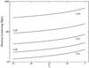 |
Fig. 1 Evolution of the first five Lyman horizons in comoving Mpc as a function of the emission redshift. The horizon labeled Lyn is the maximal distance a photon emitted just below Ly(n + 1) can travel. |
The existence of these Lyman horizons around primordial sources during the early EoR (while the Wouthuysen-Field coupling is not yet saturated) leads to discontinuities in their Lyα flux profiles, which could create similar features in the brightness temperature profiles and maps. In order to answer this question quantitatively, we have to consider a full modeling of the Lyα pumping in a realistic numerical simulation of the EoR.
4. Numerical methods
We simulated cosmological reionization as a three-step process. First, a dynamical simulation was run using GADGET2 (Springel 2005). Snapshots of the simulation were taken at regular intervals. The interval is given in terms of the scale factor: Δa = 2-10. Then the Monte-Carlo 3D radiative transfer code LICORICE (Semelin et al. 2007; Baek et al. 2009; Iliev et al. 2009) was used to compute the ionizing continuum radiative transfer. We used two different dynamical simulations. The first one simulates a (100 h-1 Mpc)3 volume with 2 × 2563 particles and assumes WMAP3 data alone cosmological parameters: Ωm = 0.24, ΩΛ = 0.76, Ωb = 0.042, h = 0.73 (Spergel et al. 2007). The source modeling (stellar sources, Salpeter IMF, with masses in the range 1–120 M⊙) and detailed reionization scheme is described in Baek et al. (2010), where a detailed analysis of the reionization history can be found. The second simulation is a box of size 200 h-1 Mpc, with 2 × 5123 particles, so that the mass resolution is the same as in the first one. It assumes the more recent WMAP7+BAO+H0 cosmological parameters: Ωm = 0.272, ΩΛ = 0.728, Ωb = 0.0455, h = 0.704 (Komatsu et al. 2011). Finally, the Lyman-line radiative transfer part of LICORICE is used as a second post-process to study the Wouthuysen-Field effect, determine the spin temperature, and calculate the differential brightness temperature of the 21 cm signal of neutral hydrogen. In order to do so, we interpolated the output of the two reionization runs on a 2563 (5123) grid for the 100 h-1 (200 h-1) Mpc simulation respectively. In both cases, we emitted 1.6 × 10⁹ Lyman-band photons between each pair of snapshots. We emphasize that the full radiative transfer in the lines is computed up to Lyϵ. Using an isotropic r-2 profile around the sources would be much easier and faster. However, it has been shown that using the real, local Lyα flux is important at early redshifts for ionization fractions smaller than ~10%, when the Lyα coupling is not yet full (Chuzhoy & Zheng 2007; Baek et al. 2009).
The implementation of radiative transfer for the higher-order Lyman-series lines is similar to the Lyα radiative transfer described in Semelin et al. (2007) and Baek et al. (2009). Important modifications are listed here:
-
1.
We now consider photons with frequencies in the range [να,νζ] to include radiative transfer of the first five Lyman resonances (Lyα – Lyϵ). A “flat” spectrum is assumed in this frequency range, i.e. every frequency has the same probability to be drawn8. We emit 1.6 × 10⁹ photons between each pair of snapshots.
-
2.
When calculating the optical depth of the propagating photon, the Lyn scattering cross-section is given by the Lorentzian profile:
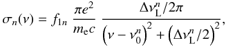 (12)with f1n the Lyn oscillator strength,
  the line center frequency, and
  the natural line width. Note that for photons whose frequency lies between Lyn and Ly(n + 1), we consider the possibility for scattering not only in the Lyn line wing, but also in the Ly(n + 1) line wing. However, we find that scatterings in the Ly(n + 1) line wing are rare and can safely be neglected.
 -
3.
When a diffusion occurs in the Lyn (n > 2) line, we consider the probability for cascading to Lyα. The probability for a Lyn photon to cascade is given by the value p = 1 − Pnp → 1s, where Pnp → 1s is the simple diffusion probability from n to the ground state (Pritchard & Furlanetto 2006). If the photon is not cascading, it is scattered by the atom.
-
4.
For cascading photons, we take into account the recycling fraction frecycle of radiative cascades that end in a Lyα photon emission. This fraction is zero for photons redshifting toward Lyβ and about 1/3 for photons redshifting toward Lyn, with n ≥ 4 (Hirata 2006; Pritchard & Furlanetto 2006). The remaining radiative cascades do not contribute to the Wouthuysen-Field effect because they end in the 2s level, from which they can reach the ground state only with a forbidden 2γ-decay. We computed scatterings until photons cascade or redshift within two thermal linewidths of a Lyn line center. At that distance from the center, given the thickness of the Lyn lines, photons are assumed to scatter without spatial diffusion and initiate a radiative cascade on the spot.
-
5.
Photons emitted below Lyβ that reach the Lyα resonance undergo τGP diffusions until they redshift out of the line, with
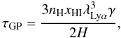 (13)where nH is the proper number density of hydrogen, λLyα the Lyα wavelength, and γ = 50 MHz the half width at half-maximum of the Lyα resonance. Typical values are τGP ~ 106 at z ~ 10. On the other hand, cascading photons are injected in the center of the Lyα line9 and thus undergo
  diffusions.
In Baek et al. (2009), the photon propagation was stopped at ten thermal linewidths of the Lyα line center. Indeed, at that distance from the center, the photon mean free path is much less than 1 physical kpc, assuming standard density and temperature conditions for the redshifts of interest. However, the mean free path is about 4 physical kpc at ten thermal linewidths of the Lyϵ line center. We thus decided to stop the photon propagation at two thermal linewidths, where the mean free paths are much shorter: ~10-5 and ~7 × 10⁻⁴ physical kpc for Lyα and Lyϵ photons respectively.
Note that we consider that Lyα heating is negligible (Pritchard & Furlanetto 2006; Furlanetto & Pritchard 2006). In a recent paper, Meiksin (2010) studies heating by higher-order Lyman-series photons and obtains heating rates as high as several tens of degrees per Gyr. However, we did not take this process into account because our work concentrates on the very early phases of the reionization epoch. For the same reason, we completely neglected the effect of dust. While dust may play a significant role in Lyman-line radiative transfer during the later stages of the EoR, this is not expected in the beginning of the EoR and we considered a fully dust-free universe.
5. Results
5.1. 3D power spectra
The 3D power spectrum has been widely used as an efficient probe of the δTb fluctuations. However, we will show that this analysis tool cannot help us in detecting Lyman horizons in our simulated data. In Fig. 2 the δTb 3D power spectrum of our fiducial 200 h-1 Mpc simulation (solid line) is compared at z = 11.05 with the power spectrum of another simulation that does not take into account higher-order Lyman-series radiative transfer for the computation of δTb (dotted line). More precisely, we propagate in the latter run the same number of photons, but this time in the interval [να,νβ]. Arrows indicate the wavenumbers corresponding to the predicted sizes of the Lyγ, Lyδ and Lyϵ horizons, as given by Eq. (11). The redshift z = 11.05 has been chosen because, as we will demonstrate later, this is when other analysis tools provide the best detection of the Lyman horizons. Also, the Hii bubbles at that moment in the simulations are numerous enough to have reliable statistics. As a consequence, the 3D power spectrum is expected to have a trustworthy shape and to be little affected by boxsize effects. On scales greater than the horizons, both spectra are very close to each other. The gain in power, compared with the fiducial simulation, on scales shorter than the Lyman horizons, is caused by the combination of (i) the fact that, compared with the fiducial simulation, we do not loose any photons in the radiative cascades, and (ii) the r-2.3 profile of Pα on small scales owing to Lyα wing scatterings (Semelin et al. 2007; Chuzhoy & Zheng 2007). Note that the power spectrum shown in this work does not look like theoretical predictions (see e.g. Naoz & Barkana 2008). We conclude from Fig. 2 that the two spectra have almost exactly the same shape, which clearly illustrates the inability of 3D power spectra to help us in detecting Lyman horizons.
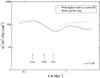 |
Fig. 2 Power spectrum of δTbat z = 11.05 for the fiducial 200 h-1 Mpc simulation (solid line) and for a simulation neglecting higher-order Lyman-series radiative transfer (dotted line). The wavenumbers corresponding to the size of the three horizons are indicated. |
5.2. Lyman horizons around individual sources
Figure 3 shows the spherically averaged xα profile at z = 13.42 around the first source of the 100 h-1 Mpc simulation that appears at z = 14.06. The dotted line is the profile obtained when calculating radiative transfer including the Lyα resonance only. In other words, this neglects the contribution of radiative cascades to the total Lyα flux. The dashed line is the result of the correct radiative transfer calculation, including the five Lyman resonances from Lyα to Lyϵ, but without considering the effect of backreaction. Finally, the solid thick line is the correct averaged xα profile, with both Lyn radiative transfer and backreaction. The reason why there is no Lyβ horizon is related to the selection rules forbidding Lyβ photons to convert to Lyα photons. We clearly observe discontinuities in the xα coefficient profile at the predicted positions.
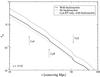 |
Fig. 3 Spherically averaged profile of the coupling coefficient for Lyα pumping xα at z = 13.42 around the first light source in the 100 h-1 Mpc simulation. The correct profile is represented by the thick solid line, while the other two neglect backreaction (dashed line) or radiative transfer for the higher-order Lyman-series lines (dotted line). As expected, we observe steep decreases in the value of the profile at radii corresponding to the predicted Lyγ, Lyδ and Lyϵ horizons (shown by arrows). |
The corresponding profile for the differential brightness temperature is given in the upper panel of Fig. 4, using the same notation as in Fig. 3. Inside the tiny Hii bubble, i.e. in the first few comoving Mpc around the source (not shown in the figure), the signal is in emission. But outside this very small ionized region, the gas kinetic temperature is clearly lower than the CMB temperature at this early redshift. For that reason, the 21 cm signal appears in absorption. It reaches a minimal value of ~–190 mK at 4.3 comoving Mpc and is as large as about –60 mK at 10 comoving Mpc from the source. Inclusion of higher-order Lyman-series radiative transfer leads to a significant increase by 25% of  at 10 comoving Mpc compared to the case where only Lyα radiative transfer is considered. Because the Wouthuysen-Field effect is dominant for determining the spin temperature, the discontinuities in the Lyα flux translate into similar discontinuities in the differential brightness temperature profile. At this redshift, decreases by about 5 mK, 2 mK and 0.2 mK at the Lyϵ, Lyδ and Lyγ horizon locations respectively. This plot also shows the importance of taking into account backreaction for the correct computation of the spin temperature. Indeed, the box-average kinetic temperature is ⟨Tk⟩ = 4.63 K at z = 13.42, and at such a low temperature the backreaction correction factor is about 0.6. In the lower panel of Fig. 4 we plot the gradient of the spherically averaged profile. Steep decreases in the temperature profile at the positions of the Lyman horizons result in prominent peaks in its gradient that make these horizons even easier to detect.
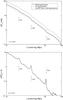 |
Fig. 4 Upper panel: spherically averaged profile of the differential brightness temperature at z = 13.42 around the first light source in the 100 h-1 Mpc simulation. The same notation is used as in Fig. 3. Note that we plot the opposite value of δTb. Lower panel: gradient of the spherically averaged profile. |
The most important conclusion from Fig. 4 is that the different steps in the xα profile at the Lyman horizons correspond to similar, clearly seen decreases in the differential brightness temperature profile.
We show in Fig. 5 a map of the quantity − δTb × r2 around the same source at the same redshift z = 13.42 with r the distance to the source center. Mapping this quantity enhances visualization. Indeed, from Eqs. (2) and (6), and since10xα ∝ r-2, it can easily be shown that δTb is also proportional to r-2. Mapping the product − δTb × r2 will thus straighten up the radial profiles, making the horizons more apparent. The slice thickness is 2 h-1 Mpc and the map scale is logarithmic. The three spherical, concentric horizons are marked with white, yellow and red arrows for the Lyϵ, Lyδ and Lyγ discontinuities respectively. On this map, the Lyδ horizon is particularly obvious. Note the perfectly spherical shape that characterizes these features.
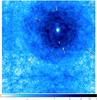 |
Fig. 5 Map of the quantity − δTb × r2 at z = 13.42, with r the distance to the source center, in arbitrary units. The Lyϵ, Lyδ and Lyγ horizons are marked with white, yellow and red arrows respectively. The size of the box is 100 h-1 Mpc and the slice thickness is 2 h-1 Mpc. The color scale is logarithmic. |
5.3. Effect of the nearby sources
From Figs. 3 to 5 we are able to conclude that the existence of Lyman horizons around the first light sources create similar features in the 21 cm signal at the very beginning of the EoR. However, these weak discontinuities, whose amplitude is only a few mK, will be progressively affected by the contribution of other nearby sources located closer than the ~ 50 comoving Mpc corresponding to the farthest Lyγ horizon. Also, Lyman photons emitted between Lyα and Lyγ by more distant sources can travel more than 50 comoving Mpc, and thus are likely to reach the outskirts of many other sources. The increasing influence of the other UV emitters on the brightness temperature profile of an individual source is shown in Fig. 6 for the 100 h-1 Mpc simulation box, from z = 13.22 to z = 11.64. This redshift interval is covered by ten snapshots and there are six emitting cells at z = 13.22, 15 at z = 12.66, 38 at z = 12.13, and 86 at z = 11.64. Early in the simulation, the three Lyman horizons are clearly seen as prominent peaks in the gradient of the temperature profile (upper left panel). Later, as the influence of the other sources becomes stronger, fluctuations in the profile grow until they reach the same amplitude as the horizons. At the beginning of this process, some of the horizon peaks are still observable (upper right and lower left panels), but after a certain time they are not distinguishable anymore (lower right panel). We find that for this particular simulation the Lyϵ and Lyδ horizons are observable during a redshift interval Δz ~ 2 and that the size of these discontinuities is about 2–4 mK. The Lyγ horizon is visible for a shorter period Δz < 1.5.
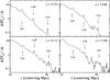 |
Fig. 6 Gradient of the spherically averaged profiles of the differential brightness temperature around the first light source appearing at z = 14.06 in the 100 h-1 Mpc simulation. The four panels show the profile at different redshifts, from z = 13.22 to z = 11.64. At each redshift, arrows show the predicted position of the Lyϵ, Lyδ and Lyγ horizons. The Lyϵ and Lyδ horizons can be detected during a redshift interval Δz ~ 2. The fainter Lyγ horizon is visible for a shorter period Δz < 1.5. |
The size of our simulation box can also be important in this attenuation process. Because of the periodic boundary conditions, a photon emitted, say, between Lyα and Lyβ can travel a distance greater than the box size, resulting in a self-contamination of the Lyα flux. Also, the smaller the simulation box, the more homogeneous is the distribution of sources around any given point in the box. In order to reduce these effects, we considered the larger, 200 h-1 Mpc simulation and find that despite the larger volume, the Lyman horizons around the first source of the simulation are observable during about the same redshift range as for the first source in the 100 h-1 Mpc simulation: Δz ~ 2 for the Lyϵ and Lyδ discontinuities, Δz ~ 1.5 for the Lyγ step. These are maximal intervals and sources lighting up later will have their horizons observable for a reduced period. As an example, the seventh source in the 200 h-1 Mpc simulation, appearing at z = 13.03, has Δz ≈ 1.2−1.5 for Lyϵ and Lyδ, and the Lyγ horizon can be detected in the first few snapshots only.
The Lyϵ and Lyδ horizons are thus the best candidates for detection, the latter one being visible a little bit longer. The Lyγ discontinuity is weaker because of the r-2 scaling of the Lyα flux, and is thus more sensitive to the influence of the other sources.
The growing fluctuations appearing in the spherically averaged temperature profiles clearly originate from the Lyα background that develops as more and more sources light up. At first sight, density or gas temperature fluctuations could also be suspected (see Eq. (6)). We thus ran test simulations in which we computed δTb assuming a perfectly homogeneous and isothermal IGM in the Lyman radiative transfer post-processing phase. The density was chosen to be the critical density and the gas kinetic temperature was assumed to be equal to the box-averaged value of the normal run. In this way, only the Lyα flux was likely to let δTbvary from one point to the next. The results of this test showed that the Lyman discontinuities are not seen for a significantly longer period than in the standard case. Indeed, we were able to identify the three horizons in a few more snapshots only, and we conclude that the density and temperature anisotropies around the source are not responsible for the disappearance of the Lyman features. A final possibility in explaining the vanishing of the Lyman steps is Monte-Carlo noise. Indeed, the total number of photons per snapshot is constant, but the source number grows quickly. As a result, the number of photons per source decreases very rapidly. However, using very expensive simulations with ten times more photons between each pair of snapshots (16 × 109) in both the 100 h-1 and 200 h-1 Mpc simulations results in undistinguishable radial profiles. We thus clearly demonstrated that the Lyman horizons disappear around individual sources because of the growing influence of the Lyα flux of the nearby sources.
5.4. Stacking
In order to extend the detectability of the Lyman steps to lower redshifts, we considered a stacking technique. This allows one to smooth the fluctuations present in the individual profiles and to strengthen the visibility of the horizon steps. As an example to illustrate the efficiency of this method, we stacked the δTb radial profiles around all the cells that contain sources in the interpolation grid of the 200 h-1 Mpc simulation at z = 11.05, when the Lyman horizons are undetectable around the vast majority of the individual sources. For some sources, small features are seen at the predicted horizon positions, but are indiscernible from fluctuations of similar amplitude. At this redshift we find 1433 source-containing cells. The individual profiles are simply added and the result is divided by the number of cells we are considering11. Figure 7 shows the gradient of the stacked profile. The presence of the Lyϵ and Lyδ horizons is now obvious.
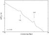 |
Fig. 7 Gradient of the stacked δTb radial profile at z = 11.05 for the 200 h-1 Mpc simulation. The stacked profile is obtained by averaging the individual profiles of all the source-containing cells at this redshift. This method allows us to detect the Lyϵ and Lyδ horizons, whose predicted positions are indicated by arrows. |
We find that this method allows us to detect these two discontinuities unambiguously down to redshifts close to 10. Interestingly however, the stacking method does not provide good results for the smaller simulation. We believe that this comes from the number of source-containing cells being about five times smaller in the 100 h-1 Mpc run at a given redshift. This has the consequence that the number of profiles that are averaged is not enough to smooth the individual fluctuations.
5.5. Detectability
We will now examine the possibility for detecting the Lyman horizons with the planned Square Kilometre Array. To this end we have to include both the instrument resolution and noise in our simulated data. We chose the noise power spectrum given by Eq. (12) of Santos et al. (2011), which models the resulting noise after the foregrounds were removed:  (14)where k is the wavenumber, θ the angle between the wave vector and the line of sight, r(z) the comoving distance to redshift z, y a conversion factor between frequency intervals and comoving distances, λ the observation wavelength, Dmax the maximum baseline, Tsys the system temperature, t0 the total observation time, and Atot the total collecting area. Following Santos et al., we use Dmax = 10 km, t0 = 1000 h and a system temperature modeled by their Eq. (13) as the sum of the receiver noise temperature (assumed to be 50 K) and the sky temperature (dominated by the Galactic synchrotron emission):
  (15)We computed the total collecting area using the sensitivity value of 4000 m2/K, in agreement with the design reference for the instrument. Following these authors, we also used 70% of Atot in the noise calculation, considering that the rest of the collecting area is used for point source removal and calibration.
Figure 8 illustrates the dramatic effect that noise may have on the detectability of Lyman horizons. The plotted example shows the gradient of the δTb radial profile around the first source of the 200 h-1 Mpc simulation at z = 12.84, with (dotted line) and without (solid line) noise. While the Lyϵ and Lyδ horizons are clearly detected in the noise-free profile, this is no longer true when noise is added.
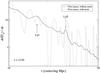 |
Fig. 8 Gradient of the δTb profile around the first source appearing in the 200 h-1 Mpc simulation at z = 12.84, with (dotted line) and without (solid line) SKA-like noise. |
However, the field of view (FoV) subtended by our simulation (less than 3 deg2 in the range z = 11 − 14) is much smaller than probable SKA fields of view. If the ratio between both fields is N, then noise will be reduced in the stacking procedure by a factor  larger for the SKA FoV than for the simulation FoV. We will here consider a field of view of 400 deg2 for the SKA. To simulate the efficiency of the stacking procedure for such a large field of view, we decreased the noise level in the simulation FoV by the appropriate factor. That we stacked over the volume of our simulation cube is not problematic in this analysis. Indeed, a short calculation shows that the full length of our 200 h-1 Mpc simulation represents a redshift difference Δz ~ 1.5, which corresponds to a ~ 6% difference in the horizon sizes at z ~ 13, according to Eq. (11). For example, this represents 1.6 comoving Mpc for Lyδ, or about 0.5′.
The most limiting factor will probably be the resolution of the instrument. The proposed SKADS-SKA implementation for observations between 70 MHz and 450 MHz suggests a 5 km-diameter core12. This gives a resolution worse than 2′ in the redshift range z = 11 − 14 relevant for our study. In order to mimic the effect of the limited instrumental resolution, we applied a 3D13 Gaussian smoothing with a FWHM equal to the resolution. We compare in Fig. 9 a map at z = 11.05 of the full-resolution, noise-free simulated data (left panel) with the same field when one includes noise and convolution with the appropriate resolution (right panel). The full-resolution map shows a characteristic signature of the early EoR 21 cm signal in the vicinity of the sources, with practically spherical Hii bubbles being surrounded by absorption regions with deep δTb local minima. On the other hand, only some of the largest bubbles are still detected in the convolved map. This will have an influence on the identification and localization of the first sources, and hence on attempts to observe Lyman horizons. Also, the limited resolution of the future observations will cause a blurring of the small discontinuities we aim to detect.
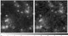 |
Fig. 9 Maps of δTb at z = 11.05. The slice is 200 h-1 Mpc on a side and has a thickness of 2 h-1 Mpc. The scale, in units of mK, is linear. The left panel shows our simulated data cube at full resolution. The right panel shows the effect of instrumental noise and instrumental resolution. At that redshift, the latter is slightly larger than 2′. |
Finding an algorithm to efficiently detect the Hii bubbles in the convolved maps will be the subject of a future paper. Here, we tackle the question of pinpointing the source positions on the sky beyond the resolution accuracy, which could leave its mark on the stacking procedure, in the following way. Instead of using the exact source position when building the stacked profile, we randomly distribute its location inside a sphere centered on the exact position. The diameter of that sphere corresponds to the SKA resolution at the considered redshift. Figure 10 shows the gradient of the stacked profile assuming the observation strategy described above (thick solid line), compared to the case without noise and with full resolution, and in which the position of the sources is perfectly known (dotted line). The important field of view allows us to significantly reduce the effect of the noise, but the 2′ resolution has a dramatic effect on the Lyman horizons, which are completely wiped off. The dashed line shows that with a 1′ resolution (10 km core), the Lyδ horizon is detected as a wide and weak hump. In order to maximize the detection probability, we assumed here perfect foreground removal and chose a redshift (z = 13.42) at which the Lyman horizons are not yet contaminated by the other nearby sources. We deduce from this figure that detection of the Lyman horizons in the early phases of the EoR using SKA observations will probably be possible only with a 1′ resolution.
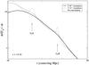 |
Fig. 10 The thick solid (thin dashed) line shows the gradient of the δTb stacked profile in the 200 h-1 Mpc simulation at z = 13.42, with SKA-like noise, assuming a field of view of 400 deg2, and a 2′30″ (1′15″) resolution. For comparison, we also show the gradient of the δTb stacked profile at the same redshift without noise nor resolution effect (dotted line). |
6. Discussion and conclusions
We studied the effects of higher-order Lyman-series radiative transfer on the differential brightness temperature of the 21 cm signal of neutral hydrogen during the early stage of the EoR. This signal was computed in the presence of inhomogeneous Wouthuysen-Field effect using the Monte-Carlo 3D radiative transfer code LICORICE. We showed that the discontinuities in the Lyα flux radial profile of the first light sources, caused by the existence of discrete Lyman horizons, lead to similar features in the differential brightness temperature profile.
We found that the Lyϵ and Lyδ horizons are detected in our simulations around individual sources during a redshift interval Δz ~ 2 after the first source lights up. Later, the Lyα flux at a given point has a growing smooth background component owing to the cumulative contribution of the other sources, and the Lyman steps fade away. However, we showed that stacking the individual profiles significantly increases the visibility period (Δz ~ 4).
An important caveat has to be mentioned here. We have considered in our simulations purely stellar sources. However, it should be kept in mind that considering an important contribution from quasars would result in the Wouthuysen-Field effect being significantly induced by Lyα photons coming from collisional excitation of hydrogen atoms by secondary electrons produced by X-rays. If an important part of the total number of Lyα photons is not coming from redshifting and cascading photons, the interesting features in δTb we discussed in this work would be more difficult to extract.
On the other hand, let us note that the size of the Lyman discontinuities could increase if the number of Lyα photons from radiative cascades is enhanced. In a recent paper, Meiksin (2010) claims that the number of these photons could be up to 30% higher than previously considered. In this case, the size of the steps in the xα profile would increase interestingly, together with the size of the corresponding δTb discontinuities.
Detections of these discontinuities would be of first importance for two reasons. First, these features would be very interesting for researchers involved in foreground removal. Indeed, removing the much brighter foregrounds (Galactic synchrotron and free-free emission, extragalactic sources, ionospheric distortions) will be a serious challenge for future 21 cm observations. But Lyman horizons are structures whose size is precisely known at a given redshift (or frequency), and for that reason positive detections would ensure that the laborious removal task has been correctly handled. The second reason is the possible use of these horizons as standard rulers, as was noted by Pritchard & Furlanetto (2006).
When assessing the question of detecting Lyman horizons with the planned Square Kilometre Array by taking into account the reference implementation and design, we found that this detection will be very challenging. Indeed, the horizons are not detected with a 2′ resolution. A 1′ resolution may allow us to detect the Lyδ horizon.
For an interesting discussion about the redshift at which reionization is complete, as deduced from the spectra of high redshift quasars, see Mesinger (2010).
Given the narrowness of this frequency range, the use of a realistic non-flat spectrum results in minor differences, as we checked using blackbody spectra with three different effective temperatures: 5 × 10⁴ K, 105 K, and 1.5 × 10⁵ K. Chuzhoy & Zheng (2007) also showed that the spectral slope of the source does not have a strong influence on the slope of the scattering-rate profile.
Indeed, Furlanetto & Pritchard (2006) noted that even if the first absorption is well blueward of the Lyman-series line center, the intermediate states of the atom during the radiative cascade have narrow natural widths.
More precisely, taking wing scatterings into account slightly steepens the profile on small scales, as noted above (Semelin et al. 2007; Chuzhoy & Zheng 2007).
We can safely ignore that the stacked sources have different peculiar velocities perpendicular to the line of sight. Indeed, a rapid estimation shows that a peculiar velocity about 300 km s-1 leads to a redshift difference Δz = (1 + z) v/c ~ 10-2. As shown in Fig. 1 and Eq. (11), this results in completely negligible differences in the horizon sizes.
For simplicity reasons, we consider the same resolution in the frequency direction as in the other two spatial directions.
Acknowledgments
We are grateful to J. Uson for helpful discussion. We also thank the anonymous referee for his/her insightful comments. This work was realized in the context of the LIDAU project. The LIDAU project is financed by a French ANR (Agence Nationale de la Recherche) funding (ANR-09-BLAN-0030). P.V. acknowledges support from a Swiss National Science Foundation (SNSF) post-doctoral fellowship. This work was performed using HPC resources from GENCI-[CINES/IDRIS] (Grant 2011-[x2011046667]).
References
- Baek, S., Di Matteo, P., Semelin, B., Combes, F., & Revaz, Y. 2009, A&A, 495, 389 [NASA ADS] [CrossRef] [EDP Sciences] [Google Scholar]
- Baek, S., Semelin, B., Di Matteo, P., Revaz, Y., & Combes, F. 2010, A&A, 523, A4 [NASA ADS] [CrossRef] [EDP Sciences] [Google Scholar]
- Barkana, R., & Loeb, A. 2004, ApJ, 609, 474 [NASA ADS] [CrossRef] [Google Scholar]
- Barkana, R., & Loeb, A. 2005, ApJ, 626, 1 [NASA ADS] [CrossRef] [Google Scholar]
- Bouwens, R. J., Illingworth, G. D., Labbe, I., et al. 2011a, Nature, 469, 504 [NASA ADS] [CrossRef] [PubMed] [Google Scholar]
- Bouwens, R. J., Illingworth, G. D., Oesch, P. A., et al. 2011b, ApJ, accepted [arXiv:1006.4360] [Google Scholar]
- Chuzhoy, L., & Zheng, Z. 2007, ApJ, 670, 912 [NASA ADS] [CrossRef] [Google Scholar]
- Ciardi, B., & Madau, P. 2003, ApJ, 596, 1 [NASA ADS] [CrossRef] [Google Scholar]
- Ciardi, B., Ferrara, A., & White, S. D. M. 2003a, MNRAS, 344, L7 [NASA ADS] [CrossRef] [Google Scholar]
- Ciardi, B., Stoehr, F., & White, S. D. M. 2003b, MNRAS, 343, 1101 [NASA ADS] [CrossRef] [Google Scholar]
- Fan, X., Carilli, C. L., & Keating, B. 2006, ARA&A, 44, 415 [NASA ADS] [CrossRef] [Google Scholar]
- Field, G. B. 1958, Proc. I. R. E., 46, 240 [Google Scholar]
- Furlanetto, S. R. 2006, MNRAS, 371, 867 [NASA ADS] [CrossRef] [Google Scholar]
- Furlanetto, S. R., & Pritchard, J. R. 2006, MNRAS, 372, 1093 [NASA ADS] [CrossRef] [Google Scholar]
- Furlanetto, S. R., Oh, S. P., & Briggs, F. H. 2006, Phys. Rep., 433, 181 [NASA ADS] [CrossRef] [Google Scholar]
- Gunn, J. E., & Peterson, B. A. 1965, ApJ, 142, 1633 [NASA ADS] [CrossRef] [Google Scholar]
- Harker, G., Zaroubi, S., Bernardi, G., et al. 2009, MNRAS, 397, 1138 [NASA ADS] [CrossRef] [Google Scholar]
- Hirata, C. M. 2006, MNRAS, 367, 259 [NASA ADS] [CrossRef] [Google Scholar]
- Hogan, C. J., & Rees, M. J. 1979, MNRAS, 188, 791 [NASA ADS] [Google Scholar]
- Iliev, I. T., Mellema, G., Pen, U., et al. 2006, MNRAS, 369, 1625 [NASA ADS] [CrossRef] [Google Scholar]
- Iliev, I. T., Mellema, G., Shapiro, P. R., & Pen, U. 2007, MNRAS, 376, 534 [NASA ADS] [CrossRef] [Google Scholar]
- Iliev, I. T., Whalen, D., Mellema, G., et al. 2009, MNRAS, 400, 1283 [NASA ADS] [CrossRef] [Google Scholar]
- Komatsu, E., Smith, K. M., Dunkley, J., et al. 2011, ApJS, 192, 18 [NASA ADS] [CrossRef] [Google Scholar]
- Kuhlen, M., Madau, P., & Montgomery, R. 2006, ApJ, 637, L1 [NASA ADS] [CrossRef] [Google Scholar]
- Madau, P., Meiksin, A., & Rees, M. J. 1997, ApJ, 475, 429 [NASA ADS] [CrossRef] [Google Scholar]
- Meiksin, A. 2010, MNRAS, 402, 1780 [NASA ADS] [CrossRef] [Google Scholar]
- Mellema, G., Iliev, I. T., Pen, U., & Shapiro, P. R. 2006, MNRAS, 372, 679 [NASA ADS] [CrossRef] [Google Scholar]
- Mesinger, A. 2010, MNRAS, 407, 1328 [NASA ADS] [CrossRef] [Google Scholar]
- Naoz, S., & Barkana, R. 2008, MNRAS, 385, L63 [NASA ADS] [Google Scholar]
- Pritchard, J. R., & Furlanetto, S. R. 2006, MNRAS, 367, 1057 [NASA ADS] [CrossRef] [Google Scholar]
- Santos, M. G., Silva, M. B., Pritchard, J. R., Cen, R., & Cooray, A. 2011, A&A, 527, A93 [NASA ADS] [CrossRef] [EDP Sciences] [Google Scholar]
- Scott, D., & Rees, M. J. 1990, MNRAS, 247, 510 [NASA ADS] [Google Scholar]
- Semelin, B., Combes, F., & Baek, S. 2007, A&A, 474, 365 [NASA ADS] [CrossRef] [EDP Sciences] [Google Scholar]
- Spergel, D. N., Bean, R., Doré, O., et al. 2007, ApJS, 170, 377 [NASA ADS] [CrossRef] [Google Scholar]
- Springel, V. 2005, MNRAS, 364, 1105 [NASA ADS] [CrossRef] [Google Scholar]
- Volonteri, M., & Gnedin, N. Y. 2009, ApJ, 703, 2113 [NASA ADS] [CrossRef] [Google Scholar]
- Wouthuysen, S. A. 1952, AJ, 57, 31 [NASA ADS] [CrossRef] [Google Scholar]
All Figures
|
Fig. 1 Evolution of the first five Lyman horizons in comoving Mpc as a function of the emission redshift. The horizon labeled Lyn is the maximal distance a photon emitted just below Ly(n + 1) can travel. |
| In the text | |
|
Fig. 2 Power spectrum of δTbat z = 11.05 for the fiducial 200 h-1 Mpc simulation (solid line) and for a simulation neglecting higher-order Lyman-series radiative transfer (dotted line). The wavenumbers corresponding to the size of the three horizons are indicated. |
| In the text | |
|
Fig. 3 Spherically averaged profile of the coupling coefficient for Lyα pumping xα at z = 13.42 around the first light source in the 100 h-1 Mpc simulation. The correct profile is represented by the thick solid line, while the other two neglect backreaction (dashed line) or radiative transfer for the higher-order Lyman-series lines (dotted line). As expected, we observe steep decreases in the value of the profile at radii corresponding to the predicted Lyγ, Lyδ and Lyϵ horizons (shown by arrows). |
| In the text | |
|
Fig. 4 Upper panel: spherically averaged profile of the differential brightness temperature at z = 13.42 around the first light source in the 100 h-1 Mpc simulation. The same notation is used as in Fig. 3. Note that we plot the opposite value of δTb. Lower panel: gradient of the spherically averaged profile. |
| In the text | |
|
Fig. 5 Map of the quantity − δTb × r2 at z = 13.42, with r the distance to the source center, in arbitrary units. The Lyϵ, Lyδ and Lyγ horizons are marked with white, yellow and red arrows respectively. The size of the box is 100 h-1 Mpc and the slice thickness is 2 h-1 Mpc. The color scale is logarithmic. |
| In the text | |
|
Fig. 6 Gradient of the spherically averaged profiles of the differential brightness temperature around the first light source appearing at z = 14.06 in the 100 h-1 Mpc simulation. The four panels show the profile at different redshifts, from z = 13.22 to z = 11.64. At each redshift, arrows show the predicted position of the Lyϵ, Lyδ and Lyγ horizons. The Lyϵ and Lyδ horizons can be detected during a redshift interval Δz ~ 2. The fainter Lyγ horizon is visible for a shorter period Δz < 1.5. |
| In the text | |
|
Fig. 7 Gradient of the stacked δTb radial profile at z = 11.05 for the 200 h-1 Mpc simulation. The stacked profile is obtained by averaging the individual profiles of all the source-containing cells at this redshift. This method allows us to detect the Lyϵ and Lyδ horizons, whose predicted positions are indicated by arrows. |
| In the text | |
|
Fig. 8 Gradient of the δTb profile around the first source appearing in the 200 h-1 Mpc simulation at z = 12.84, with (dotted line) and without (solid line) SKA-like noise. |
| In the text | |
|
Fig. 9 Maps of δTb at z = 11.05. The slice is 200 h-1 Mpc on a side and has a thickness of 2 h-1 Mpc. The scale, in units of mK, is linear. The left panel shows our simulated data cube at full resolution. The right panel shows the effect of instrumental noise and instrumental resolution. At that redshift, the latter is slightly larger than 2′. |
| In the text | |
|
Fig. 10 The thick solid (thin dashed) line shows the gradient of the δTb stacked profile in the 200 h-1 Mpc simulation at z = 13.42, with SKA-like noise, assuming a field of view of 400 deg2, and a 2′30″ (1′15″) resolution. For comparison, we also show the gradient of the δTb stacked profile at the same redshift without noise nor resolution effect (dotted line). |
| In the text | |
Current usage metrics show cumulative count of Article Views (full-text article views including HTML views, PDF and ePub downloads, according to the available data) and Abstracts Views on Vision4Press platform.
Data correspond to usage on the plateform after 2015. The current usage metrics is available 48-96 hours after online publication and is updated daily on week days.
Initial download of the metrics may take a while.