| Issue |
A&A
Volume 531, July 2011
|
|
|---|---|---|
| Article Number | A95 | |
| Number of page(s) | 14 | |
| Section | Extragalactic astronomy | |
| DOI | https://doi.org/10.1051/0004-6361/201116857 | |
| Published online | 21 June 2011 | |
Catching the radio flare in CTA 102
I. Light curve analysis
1
Max-Planck-Institut für Radioastronomie, Auf dem Hügel 69, 53121 Bonn, Germany
e-mail: cfromm@mpifr.de
2
Departament d’Astronomia i Astrofísica, Universitat de València, Dr. Moliner 50, 46100 Burjassot, València, Spain
3
Departament de Matemàtiques per a l’Economia i l’Empresa, Universitat de València, Av. Tarongers s/n, 46022 València, Spain
4
Department of Astronomy, University of Michigan, Dennison Building, Ann Arbor, MI 48109, USA
5
Harvard-Smithsonian Center for Astrophysics, 60 Garden Street, Cambridge, MA 02138, USA
6
Aalto University, Metsähovi Radio Observatory, 02540 Kylmälä, Finland
Received: 9 March 2011
Accepted: 4 May 2011
Context. The blazar CTA 102 (z = 1.037) underwent a historical radio outburst in April 2006. This event offered a unique chance to study the physical properties of the jet.
Aims. We used multifrequency radio and mm observations to analyze the evolution of the spectral parameters during the flare as a test of the shock-in-jet model under these extreme conditions.
Methods. For the analysis of the flare we took into account that the flaring spectrum is superimposed on a quiescent spectrum. We reconstructed the latter from archival data and fitted a synchrotron self-absorbed distribution of emission. The uncertainties of the derived spectral parameters were calculated using Monte Carlo simulations. The spectral evolution is modeled by the shock-in-jet model, and the derived results are discussed in the context of a geometrical model (varying viewing angle) and shock-shock interaction
Results. The evolution of the flare in the turnover frequency-turnover flux density (νm − Sm) plane shows a double peak structure. The nature of this evolution is dicussed in the frame of shock-in-jet models. We discard the generation of the double peak structure in the νm − Sm plane purely based on geometrical changes (variation of the Doppler factor). The detailed modeling of the spectral evolution favors a shock-shock interaction as a possible physical mechanism behind the deviations from the standard shock-in-jet model.
Key words: galaxies: active / galaxies: jets / radiation mechanisms: non-thermal / quasars: individual: CTA 102
© ESO, 2011
1. Introduction
The blazar CTA 102 (B2230+114) has a redshift of z = 1.037 (Hewitt & Burbidge 1989). It is classified as a highly polarized quasar (HPQ) with a linear optical polarization above 3% (Véron-Cetty & Véron 2003) and a V-band magnitude of 17.33. The source was observed for the first time by Harris & Roberts (1960). Kardashev (1964) reported on possible signals from an extraterrestrial civilization coming from CTA 102. Sholomitskii (1965) found the first variation in flux density for a radio source. Later observations identified CTA 102 as a quasar.
Since that time CTA 102 has been the target of numerous observations at different wavelengths. Besides the aforementioned variation in the radio flux density, CTA 102 also shows variation in the optical band. Pica et al. (1988) reported a variation range of 1.14 mag around an average value of 17.66 mag in 14 years, and an increase of 1.04 mag within two days in 1978, which is so far the most significant outburst. CTA 102 has been monitored since 1986 within the cm-observations of the Metsähovi telescope. The strongest radio flare since the beginning of the monitoring took place around 1997, and a nearly simultaneous outburst in the optical R-band was observed with the Nordic Optical Telescope on La Palma (Tornikoski et al. 1999). The source has been detected in the γ-ray regime by the telescopes CGRO/EGRET and Fermi/LAT with a luminosity, Lγ = 5 × 1047 erg/s, defining CTA 102 as a γ-bright source (Nolan et al. 1993; Abdo et al. 2009). Merlin and VLA observations at 2 GHz, 5 GHz and 15 GHz revealed the kpc-scale structure of CTA 102 which consists of a central core and two faint lobes (Spencer et al. 1989). The brighter lobe has a flux density of 170 mJy at a distance of 1.6 arcsec from the core at position angle (PA) of 143° (measured from north through east). The other lobe, with a flux density of 75 mJy, is located 1 arcsec from the center at PA − 43°. The spectral indices between 2 GHz and 5 GHz of the lobes are −0.7 for the bright and −0.3 for the other one.
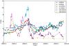 |
Fig. 1 Radio-mm light curves for CTA 102, centered around the 2006 radio flare. |
High-resolution VLBI observations at 1.4 GHz and 5 GHz resolved the central object into three components and a diffuse tail bending to the southeast. These observations provide and upper limit around 10 c (0.5 mas/yr) for the superluminal motion of the components (Bååth 1988; Wehrle & Cohen 1989). Several observations at different frequencies (for example at 326 MHz) confirmed the elongation of the source to the southeast (Altschuler et al. 1995).
Within the framework of the VLBA 2 cm-Survey (e.g., Zensus et al. 2002) and the MOJAVE1 program (MOnitoring of Jets in Active galactic nuclei with VLBA Experiments) (e.g., Lister et al. 2009a) CTA 102 has been monitored regularly, beginning in mid 1995. These intensive observations deliver a detailed picture on the morphology and kinematics of this source at 15 GHz. Kinematic analysis show apparent velocities of the features in the jet between 0.7 c and 15.40 c (Lister et al. 2009b). A multifrequency VLBI study including data at 90 GHz, 43 GHz and 22 GHz was reported by Rantakyrö et al. (2003). The results from the multifrequency VLBI observations were combined with the continuum monitoring performed at single-dish observatories at 22 GHz, 37 GHz, 90 GHz and 230 GHz. Within this multifrequency data set (November 1992 until June 1998), a major flare in CTA 102 around 1997 was confirmed. The authors could conclude that this event was connected to the ejection of a new jet feature. The same was noted by Savolainen et al. (2002). Jorstad et al. (2005) and Hovatta et al. (2009) found Lorentz factors, Γ, of 17 and 15, respectively, and Doppler factors, D, between 15 and 22 associated to this ejection. The 2006 radio flare in CTA 102 has been observed at cm − mm total flux density and multifrequency VLBI observations (Fromm 2009). The results of the the multifrequency VLBI observations will be presented in second paper.
In this work, we concentrate on the analysis of the cm − mm light curves. The organization of the paper is the following. In Sect. 2 we present the radio/mm light curves during the 2006 flare and perform the spectral analysis. The theoretical background and the fitting technique are introduced in Sect. 3. The results of this analysis are shown in Sect. 4. and are applied to the 2006 flare in CTA 102 in Sect. 5. In Sect. 6 we discuss the different models that can explain the observations.
Throughout this paper we define the optically thick spectral index as αt > 0 and the convention used for the optically thin spectral index is S ∝ ν + α, where α0 < 0. The latter can be derived from the spectral slope, s, via the relation α0 = −(s − 1)/2.
2. Observations: cm – mm light curves
For our analysis we focused on the radio flare around April 2006 and used observations spanning from 4.8 GHz to 340 GHz (see Fig. 1). The observations have been carried out by the Radio Observatory of the University of Michigan (UMRAO), the Metsähovi Radio Observatory, and the SubMillimeter Array (SMA). The average sampling time intervals and flux density uncertainties are presented in Table 1.
Average time sampling and average flux density uncertainties for the used light curves.
Figure 1 shows the total flux densities measured by the telescopes at different frequencies. The most prominent feature in the light curve is the major flare around 2006.2, best seen at 37 GHz. This feature is surrounded by smaller flares in 2005.2, 2007.6, 2008.5, and 2009.4. The light curves show the typical evolution of a flare: the flaring phenomenon usually starts at high frequencies and propagates to lower frequencies with a certain time delay of the peak, but there are also flares that develop simultaneously over a wide frequency range. The flare around 2005.0 appears nearly simultaneously at the highest frequencies (230 GHz and 340 GHz) and delayed at 37 GHz and 14.5 GHz, whereas it seems that the lowest frequencies (4.8 GHz and 8 GHz) are not affected by this event.
The main flare shows the typical evolution: it is clearly visible at all frequencies with increasing time delays towards lower frequencies. Due to the poor time sampling of the 340 GHz observations, the rise and the time shift at this frequency are not easy to determine. The remarkable double peak structure of the 230 GHz measurements is an interesting feature and will be discussed later. After the flare, the flux decreases at all frequencies, with a steeper descent at higher frequencies.
2.1. Time sampling and interpolation
To perform a spectral analysis of the light curves, simultaneous data points are needed. This was achieved by performing a linear interpolation between the flux density values from the observations. The choice of an adequate time sampling, Δt, depends on the time interval of the observations and the significance of the frequency for the determination of the peak frequency, i.e., the frequency where the spectral shape changes from optically thick to optically thin. If a too short time interval is chosen, most of the data points would be interpolated ones. On the opposite situation, if a too long time interval is chosen, most of the light curves would be smoothed. Moreover, in this case, the data are sampled inhomogeneously at the different frequency, so a compromise is required. The influence of a certain frequency on the calculation of νm can be estimated from the light curve (see Fig. 1). The turnover frequency is usually between the frequencies of the highest and second highest flux density at a certain epoch. In the case studied here, the dominating frequencies are 37 GHz and 230 GHz. From this distribution it could be concluded that an appropriate time sampling should not be significantly shorter than the observational time interval used for these frequencies. A time sampling of Δt = 0.05 yr was selected for the interpolation, corresponding approximately to the observation cadence of the 37 GHz-light curve.
The correct handling of the uncertainties in the interpolated flux densities requires knowledge of a mathematical relation describing the light curves. Since this approach is out of the scope of this paper, we assigned the maximum uncertainty of the two closest observed flux densities to the interpolated flux density. For our analysis we focused on the time interval between 2005.6 and 2006.8. The interpolation of the poorly sampled 340 GHz light curve after 2006.2 could induce artificially flat spectra. We took this fact into consideration by excluding the interpolated 340 GHz flux densities from the spectral analysis for 2006.2 < t < 2006.8.
2.2. Spectral analysis
Following (Türler et al. 2000), a synchrotron self absorbed spectrum is described by 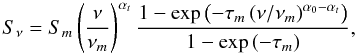 (1)where
  is the optical depth at the turnover frequency, Sm is the turnover flux density, νm is the turnover frequency and αt and α0 are the spectral indices for the optically thick and optically thin parts of the spectrum, respectively.
The observed spectra may in general be thought as the superposition of the emission from the steady state and perturbed (shocked) jet. We re-constructed this quiescent spectrum from archival data and we identified the quiet state with the minimum flux density of the low frequency light curves (4.8 − 37 GHz) around t = 1989.0 (see Fig. 2 and Table 2). The flux densities were fitted by a power law S(ν) = cqνα0 and we obtained cq = 7.43 ± 0.65 and α0 = −0.45 ± 0.04.
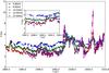 |
Fig. 2 Archival low frequency light curves for CTA 102. See insert plot for the absolute quiescent state. |
For the spectral analysis, we removed the contribution of the quiescent spectrum from the interpolated data points and applied Eq. (1). The uncertainties of the remaining flaring spectrum were calculated using the errors of the interpolated data points and the obtained uncertainties of the quiescent spectrum. During the fitting process we allowed both spectral indices, αt and α0 to vary. Figure 3 shows the result of a spectral fitting at a selected epoch applied to interpolated light curve data.
2.3. Error analysis of the spectra
Due to the non-linear nature of Eq. (1) we applied a Monte-Carlo simulation to the observed/interpolated flux densities in order to derive estimates for the uncertainties of the fitting parameters (Sm, νm, αt, and α0). Random values for each simulated spectrum were drawn from a Gaussian distribution with a mean, μ, equal to the observed flux density, S(ν), and a variance, σ, equal to the observed flux density error, ΔS(ν). In order to achieve a good statistical ensemble, up to 1000 spectra were simulated per interpolated spectrum. Each of these simulated spectra were fitted with a synchrotron spectrum (see Eq. (1)). As the expected value and uncertainty of a spectral parameter we take the mean and standard deviation of its simulated probability density distribution, respectively. The derived spectral parameters and their uncertainties are presented in Table 3.
3. Synchrotron radiation and the shock-in-jet model
In this section we review the shock-in-jet model as derived by Marscher & Gear (1985) and different modifications to it. In this review we have included the redshift dependence in the different equations where it is required. In this way, we can fit the model to observational data from any source.
3.1. Synchrotron radiation
The specific intensity from a power law distribution of relativistic electrons, N(E) = KE − s, where K is the normalization coefficient of the distribution and s the spectral slope is defined by: 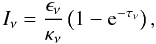 (2)where ϵν and κν are the emission and absorption coefficients, respectively, and τν is the optical depth. The emission and absorption coefficients can be written as (for details see Pacholczyk 1970):
 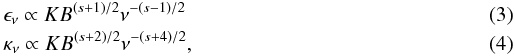 where B is the magnetic field and ν the frequency in the source frame. With this definition of the emission and absorption coefficients the specific intensity is:
 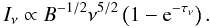 (5)Depending on the optical depth, τν, Eq. (5) describes an optically thick (τν > 1) or optically thin (τν < 1) spectrum with their characteristic shapes Iν ∝ ν5/2 and Iν ∝ ν − (s − 1)/2, respectively.
Frequencies and flux density values for the quiescent spectrum.
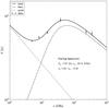 |
Fig. 3 Result of the spectral fitting to the 2006.20 data. The dashed-dotted line corresponds to the quiescent spectrum, the dashed line to the flaring spectrum, and the solid black line to the total spectrum. The values presented indicate the spectral turnover of the flaring spectrum. |
Spectral parameters (expected values) and corresponding uncertainties from the Monte-Carlo simulation.
The optically thin flux density from a jet located at luminosity distance DL, with radius R, conical geometry (half opening angle φ), constant velocity β and viewing angle ϑ is given by  (6)where
  is the solid angle, and z was the redshift. Taking into account the influence of the Doppler factor, D = Γ-1(1 − βcosϑ)-1 (see e.g., Lind & Blandford 1985), where Γ = (1 − β2) − 1/2 the Lorentz factor, Eq. (6) leads to:
  (7)The turnover frequency, defined as the frequency where the optical depth is equal to unity, can be expressed as:
  (8)The turnover flux density
  is then obtained by inserting Eqs. (8) into (7):
  (9)The equations above were successfully used to model the steady-state emission from quasars, where a decrease in the particle density N and the magnetic field B along the jet was assumed (e.g., Königl 1981). However, the observed flux densities during flares showed a more complicated behavior and could not be described by steady-state models.
3.2. Shock-in-jet model
The shock-in-jet model of Marscher & Gear (1985) studied the evolution of a traveling shock wave in a steady state jet. During the passage of the shock through a steady jet, the relativistic particles are swept up at the shock front and gain energy while crossing it. In this model, the flaring flux density is assumed to be produced by the accelerated particles within a small layer of width x behind the shock front. The width of this layer is assumed to depend on the dominant cooling process and can be approximated by x ∝ tcool, where tcool is the typical cooling time i.e., synchrotron cooling time.
3.2.1. Evolutionary stages
Compton losses:
assuming the photon energy density, uph, is higher than the magnetic energy density, ub = B2/(8π), the inverse Compton scattering is the dominant energy loss mechanism during the first stage of the flare. The width of the layer behind the shock front during this so-called Compton stage, x1, is computed to be  (10)An approximation of the photon energy density, uph, can be obtained by integrating the emission coefficient, ϵν, over the optically thin regime (νm < ν < νmax)2, which leads to
  (11)The final expression for the width of the layer behind the shock front during the Compton stage can be written as
  (12)
(12)
Synchrotron losses:
synchrotron losses become more important at the point where the photon energy density, uph, is comparable to the magnetic energy density, ub. The width of the layer x2 in the synchrotron stage can be computed by replacing uph in Eq. (10) with ub = B2/(8π) and is given by  (13)
(13)
Adiabatic losses:
radiative losses become less important in the last stage of the shock evolution. During this final stage the losses are dominated by the expansion of the source and the width of the layer, x3, is assumed to be similar to the radius of the jet  (14)The evolution of the turnover frequencies νm,i and turnover flux densities Sm,i, where i indicates the different energy loss stages (1 = Compton, 2 = synchrotron and 3 = adiabatic loss stage), can be derived by inserting the expressions for xi into Eqs. (8) and (9):
 ![\begin{eqnarray} && \nu_{m,1} \propto \left(1+z\right)^{-(s+4)/(s+5)} R^{-1/4}B^{1/4}D^{(s+3)/(s+5)}\\ && S_{m,1} \propto \left(1+z\right)^{(2s+15)/(2s+10)} D_{\rm L}^{-2} R^{11/8}B^{1/8}D^{(3s+10)/(s+5)}\\ && \nu_{m,2} \propto \left(1+z\right)^{-(s+4)/(s+5)} \left[K^2B^{s-1}D^{s+3}\right]^{1/(s+5)}\\ && S_{m,2} \propto \left(1+z\right)^{(2s+15)/(2s+10)} D_{\rm L}^{-2} R^{2}\left[K^5B^{2s-5}D^{3s+10}\right]^{1/(s+5)}\\ && \nu_{m,3} \propto \left(1+z\right)^{-1} \left[RKB^{(s+2)/2}D^{(s+2)/2}\right]^{2/(s+4)}\\ && S_{m,3} \propto \left(1+z\right)D_{\rm L}^{-2} \left[R^{2s+13}K^5B^{2s+3}D^{3s+7}\right]^{1/(s+4)}. \end{eqnarray}](/articles/aa/full_html/2011/07/aa16857-11/aa16857-11-eq119.png) Furthermore Marscher (1990); Lobanov & Zensus (1999) assumed that the evolution of K, B and D could be written as a power-law with the jet radius R (notice that in a conical jet the distance along the jet L is linearly proportional to the jet radius R, L ∝ R),
Furthermore Marscher (1990); Lobanov & Zensus (1999) assumed that the evolution of K, B and D could be written as a power-law with the jet radius R (notice that in a conical jet the distance along the jet L is linearly proportional to the jet radius R, L ∝ R),  (21)Then, a relation between the turnover flux density and the turnover frequency can be found:
 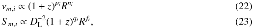 which leads to
 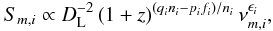 (24)where ϵi = fi/ni. The exponents fi, ni, pi and qi include the dependence with the physical quantities B, N(E), K, and D and can be written as:
 ![\begin{eqnarray} && n_1 = -(b+1)/4-d(s+3)/(s+5) \label{an1}\\ && n_2 = -[2k+b(s-1)+d(s+3)]/(s+5)\\ && n_3 = -[2(k-1)+(b+d)(s+2)]/(s+4)\label{n3}\\ && f_1 = (11-b)/8-d(3s+10)/(s+5)\\ && f_2 = 2-[5k+b(2s-5)+d(3s+10)]/(s+5)\\ && f_3 = [2s+13-5k-b(2s+3)-d(3s+7)]/(s+4)\label{f3} \\ && p_1 = -(s+4)/(s+5)\\ && p_2 = -(s+4)/(s+5)\\ && p_3 = -1\\ && q_1 = (2s+15)/(2s+10)\\ && q_2 = (2s+15)/(2s+10)\\ \label{aq3} && q_3 = 1. \end{eqnarray}](/articles/aa/full_html/2011/07/aa16857-11/aa16857-11-eq131.png) The typical evolution of a flare in the turnover frequency-turnover flux density (νm − Sm) plane can be obtained by inspecting the R-dependence of the turnover frequency, νm, and the turnover flux density, Sm, for a typical set of parameters: b = 1, s = 2.5, k = 3 (assuming an adiabatic flow, k = 2(s + 2)/3) and d = 0 (assuming constant velocity). These parameters lead to a set of exponents ni and fi, which are summarized in Table 4.
The typical evolution of a flare in the turnover frequency-turnover flux density (νm − Sm) plane can be obtained by inspecting the R-dependence of the turnover frequency, νm, and the turnover flux density, Sm, for a typical set of parameters: b = 1, s = 2.5, k = 3 (assuming an adiabatic flow, k = 2(s + 2)/3) and d = 0 (assuming constant velocity). These parameters lead to a set of exponents ni and fi, which are summarized in Table 4.
During the first stage, where Compton losses are dominant, the turnover frequency, νm, decreases with radius, R, while the turnover flux density, Sm, increases. In the second stage, where synchrotron losses are the dominating energy loss mechanism, the turnover frequency continues to decrease while the turnover flux density is constant. Both the turnover frequency and turnover flux density decrease in the final, adiabatic stage.
3.2.2. Generalization of the shock-in-jet model
Türler et al. (2000) expanded the shock-in-jet model to non-conical jets, e.g., the distance along the jet, L, is no longer a linearly proportional to the jet radius, R. This modification is expressed by R ∝ Lr with (− 1 < r < 1), which represents a collimating (r < 0) or expanding (r > 0) jet. An important implication of allowing non-conical jets (r ≠ 1) in the shock-in-jet model is the r-dependence of the evolution of the spectral parameters (b, k and d). Therefore the evolution of B, K and D along the jet is given by:  (37)Besides the modification of the jet geometry, Türler et al. (2000) parametrized the temporal evolution of the turnover frequency, νm, and the turnover flux density, Sm, using the equations of superluminal motion3
 (38)Using the definition of the apparent speed, βapp = (βsinϑ)/ (1 − βcosϑ), the bulk Lorentz factor, Γ, and the Doppler factor, D, the equation above results in
  (39)Assuming that β ~ 1 and ϑ ~ 1/Γ ≪ 1, it can be shown that Γ ∝ D (Taylor expanding cos1/Γ in the definition of D). Including the non-conical jet geometry (R ∝ Lr) the equation above can be written as
  (40)where ρ = (2dr + 1)/r. By replacing R in Eqs. (22) and (23) by (40), the temporal evolution of the turnover frequency and turnover flux density is:
 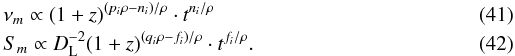 The equations above can be further simplified by replacing DL ∝ (1 + z), which leads to:
 ![\begin{equation} S_m\propto (1+z)^{\left[(q_i-2)\rho-f_i\right]/\rho}\cdot t^{f_i/\rho}. \label{tsm} \end{equation}](/articles/aa/full_html/2011/07/aa16857-11/aa16857-11-eq165.png) (43)
(43)
3.2.3. Modification of the COMPTON stage
The determination of the distance that the relativistic particles travel behind the shock front before losing most of their energy, was a crucial parameter in shock-in-jet models. Björnsson & Aslaksen (2000) presented a more accurate derivation of this distance than previous works, including the possibility of multiple Compton scattering (in the Thompson regime) during the first rising phase of the flare. In the case of first order Compton scattering, the evolution of the first stage was predicted to be less abrupt when compared to Marscher & Gear (1985). Therefore the existence of a synchrotron stage was no longer needed. The evolution of the turnover-flux density, νm, and the turnover frequency, Sm, with distance (or time) is given, within this model, by: ![\begin{eqnarray} \label{numbj} && \nu_m \propto R^{-[4(s+2)+3b(s+4)]/[3(s+12)]}\\ \label{smbj} && S_m \propto R^{-[4(s-13)+6b(s+2)]/[3(s+12)]}, \end{eqnarray}](/articles/aa/full_html/2011/07/aa16857-11/aa16857-11-eq166.png) assuming no changes in the Doppler factor and constant velocity of the shocked particles. Using the same set of parameters as in Table 4 leads to n1 = −0.9 and f1 = 0.3, resulting in a less steep slope ϵ1 = f1/n1 = −0.3 in the νm − Sm-plane which is flatter than in Marscher & Gear (1985) case.
assuming no changes in the Doppler factor and constant velocity of the shocked particles. Using the same set of parameters as in Table 4 leads to n1 = −0.9 and f1 = 0.3, resulting in a less steep slope ϵ1 = f1/n1 = −0.3 in the νm − Sm-plane which is flatter than in Marscher & Gear (1985) case.
4. Results
The spectral evolution of the 2006 radio flare in CTA 102 is presented in the turnover frequency-turnover flux density (νm − Sm) plane, shown in Fig. 4. Figures 5 and 6 display the time evolution of the spectral parameters (νm,Sm,α0, and αt).
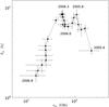 |
Fig. 4 The 2006 radio flare in the turnover frequency-turnover flux density plane. The time labels indicate the time evolution and the temporal position of local and global extrema in the spectral evolution. |
Different stages of the spectral evolution and their characteristics.
In the next paragraphs, we summarize the evolution of the event in the turnover frequency-turnover flux density plane and compare it with the standard shock-in-jet model (Marscher & Gear 1985) and later modifications to it (Björnsson & Aslaksen 2000). This information is also summarized in Table 5.
The flare started around 2005.6 with a high turnover frequency (νm ~ 200 GHz) and a low turnover flux density (Sm ~ 3 Jy). During the first 0.2 yr, the turnover flux density, Sm, increased, reaching Sm ~ 8.4 Jy, while the turnover frequency decreased to νm ~ 110 GHz. The slope of the optically thick part of the spectrum, represented by αt, steepened (0.33 to 0.78), while the optically thin spectral index, α0, steepened during the first 0.05 yr and flattened (− 1.8 to − 1.02) afterwards. The large uncertainties of the optically thin spectral index, α0, are due to the lack of data points beyond 340 GHz. The exponential relation between the turnover flux density, Sm and the turnover frequency, νm, ( , see Sect. 3.2), led to a value of ϵ = −1.21 ± 0.22.
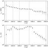 |
Fig. 5 Temporal evolution of the 2006 radio flare: top turnover frequency and bottom turnover flux density. The dashed vertical lines correspond to the time labels in Fig. 4 and indicate the extrema in the evolution. |
As mentioned in Sect. 3, the dominant loss mechanism during the first stage of flare (increasing turnover flux density while the turnover frequency was decreasing) was Compton scattering. Marscher & Gear (1985) predicted a value of ϵ = −5/2, whereas Björnsson & Aslaksen (2000) derived ϵ = −0.43 using a modified expression for the shock width (both assumed s = 2.4 and b = 1). The obtained value of ϵ = −1.21 ± 0.22 was in between these two values, but it is impossible to reproduce using the approach of Björnsson & Aslaksen (2000).
During the time interval between 2005.8 and 2006.0, involving 0.2 yr, the turnover flux density and turnover frequency decreased to Sm ~ 6.2 Jy and to νm ~ 62 GHz, respectively. The slope in the νm − Sm-plane changed to ϵ = 0.77 ± 0.11. The average optically thick spectral index reached a value αt ~ 0.82 ± 0.17 while the optically thin spectral index, α0, continued rising to −0.22. This behavior of the turnover values fits well in the adiabatic stage in the shock-in-jet model. For this stage Marscher & Gear (1985) derived an exponent ϵ = 0.69 (assuming s = 3), which is well within our value.
However, the increase of the turnover flux density starting in 2006.0, which reached a peak value of Sm ~ 8.5 Jy in 2006.3, cannot be explained within the frame of the shock-in-jet model. Its behavior, though, resembles that expected from a Compton stage (ϵ = −0.99 ± 0.46). The spectral indices during this stage were roughly constant, αt = 1.33 ± 0.27 and α0 = −0.26 ± 0.13.
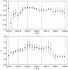 |
Fig. 6 Temporal evolution of the optically thin (α0, top) and thick (αt, bottom) spectral indices for 2006 radio flare. The dashed vertical lines corresponds to the time labels in Fig. 4 and indicate the extrema in the evolution. |
After 2006.3, the turnover flux density and turnover frequency decreased. This last phase could be understood as an adiabatic stage and the power law fit in the νm − Sm-plane led to an ϵ = 1.24 ± 0.10. The optically thin spectral index was nearly constant, α0 = −0.46 ± 0.21 while the evolution of the optically thick spectral index, αt, could be divided into two parts: αt = 0.96 ± 0.28 until 2006.5 and αt = 0.26 ± 0.18 after.
Our results show no evidence for a synchrotron stage, characterized by a nearly constant turnover flux density, Sm, while the turnover frequency, νm, is decreasing (ϵ = −0.05 for s = 2.4 and b = 1, Marscher & Gear 1985).
The first hump in the evolution of the flare in the νm − Sm-plane (2005.6 < t < 2006.0) fulfills, despite no evidence for a synchrotron stage, the phenomenological requirements of the shock-in-jet model of Marscher & Gear (1985). However, the evolution after 2006.0 did not follow the predicted evolution. The turnover flux density and the turnover frequency should continue decreasing. But their behavior mimicked the evolution of a Compton stage (2006.0 < t < 2006.3) and the one of an adiabatic stage (2006.3 < t < 2006.8). Considering these points, we decided to model the evolution of the 2006 flare in CTA 102 according to the standard shock-in-jet model (Marscher & Gear 1985) including a second Compton and adiabatic stage. This decision is evaluated in Sect. 6.
5. Modeling the 2006 radio flare
In this section we present the results of applying the shock-in-jet model and the fitting technique to the observed spectral evolution of the 2006 radio flare in CTA 102.
5.1. Fitting technique
We used a multi-dimensional χ2-optimization for deriving a set of parameters that fit the spectral evolution of the different stages. Our approach consists on fitting the temporal evolution of the spectral turnover values, νm and Sm using Eqs. (41) and (43) and the definition of the spectral exponents (see Eqs. (25) − (36)). The proportionalities in Eqs. (41) and (43) can be removed by introducing the constants cνm,i and cSm,i, which reflect logarithmic shifts of the turnover frequency and flux density and depend on the intrinsic properties of the source and flare, having no further importance for our study. From the observed values,  and
and  (i indicating the radiation loss stage, and j indicating the position among the total number of points in the stage, q, so that j = 1···q), the proportionality constants can be derived as:
 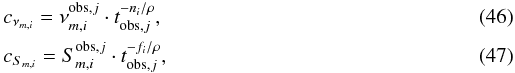 where tobs,j is the time in the observers frame. Using these definitions, the constant for the spectral evolution in the νm − Sm plane (see Eq. (24)) yields:
  (48)From Eqs. (25) − (36), (41), and (43), we see that there are 5 parameters (b, s, k, d, and r) that describe the whole spectral evolution, although they have different values at each stage. Starting from basic physical principles, we used boundaries for the different parameters to avoid unphysical results. These boundaries are listed in Table 6.
Range for spectral parameters allowed to vary in the fits to the observed spectrum for all stages.
The negative values for parameter d stand for the possibility for an increase in the Doppler factor, D, with radius. Regarding r, negative values correspond to collimation, i.e., a decrease of the jet radius, and positive values correspond to an expansion process.
On top of the listed limitations, the evolution of the optically thin spectral index, α0, can be used to provide estimates of the parameter s = 1−2α0. Marscher & Gear (1985) used a lower limit of s = 2 to keep the shock non-radiative. A flatter spectral slope, e.g., s < 2, would increase the amount of high energy electrons, which will dominate the energy density and the pressure in shock. Since these particles suffer radiative cooling, their energy losses would affect the dynamics leading to a radiative shock.
As mentioned before, allowing non-conical jet expansion (r ≠ 1) also affects the boundaries for the spectral parameters k and d presented in Table 6, which depend on the value of r in the non-conical case. Note that this should be taken into account in order to properly interpret the evolution of the physical parameters with distance to the core.
We developed a least-square algorithm to fit the three different radiation loss stages (Compton, synchrotron, or adiabatic, or combinations of them) to the observed evolution using one single set of parameters. During the optimization of χ2 all observed data points were used for calculating the constants cνm,i and cSm,i, which allows for an improved χ2. This technique allowed us to test and analyze different possible scenarios (b, s, k, d, and r).
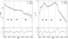 |
Fig. 7 Temporal spectral evolution of the 2006 radio flare in CTA 102 left: turnover frequency; right: turnover flux density. The lower panels show the residuum for the fits |

Best fit values for spectral evolution modeling of the 2006 radio flare in CTA 102, parameters b, d, s, kr and t.
5.1.1. Spectral evolution before 2006.0
The spectral evolution until 2006.0 followed approximately the standard evolution described by the shock-in-jet model. However, we have not found evidence for a plateau phase of turnover flux density, Sm, neither after the first Compton stage nor after the second Compton-like stage. Therefore, we excluded the synchrotron stage from our modeling using a direct transition from the Compton to the adiabatic one. The result of this modeling is presented in Table 7 as model C1A1.
5.1.2. Spectral evolution between 2006.0 and 2006.3
The second peak in the Sm − νm plane shows a similar behavior to a Compton stage, as stated above. Therefore, we applied the equations of the Compton stage to the spectral evolution between 2006.0 and 2006.3. Since the Compton stage can be explained within a 4-dimensional parameter space (note that it does not depend on parameter k, Eqs. (25) − (36)), we selected carefully a physically meaningful combination of parameters.
Boundaries for the slope of the relativistic electron distribution, s, can be derived by using the evolution of the optically thin spectral index of the emission  between 2006.0 and 2006.3. This evolution is shown in Fig. 6. We obtained values of smin = 1.4 and smax = 2 from the optically thin spectral indices α0 = −0.20 and α0 = −0.47, respectively.
5.1.3. Spectral evolution after 2006.3
The spectral evolution after 2006.3 shows the typical behavior of an adiabatic loss stage. Again, we used the evolution of the optically thin spectral index, α0, shown in Fig. 6, to derive limits for the parameter s. The obtained values are smin = 1.6 and smax = 2.5. This stage could be divided into two substages (before and after 2006.45) but the limited time sampling (with only three data points in the first part) forced us to perform the spectral fitting to the whole adiabatic stage.
5.2. Final model and error analysis
Table 7 lists the best fits and errors of the different stages. In the first column, we show the values for C1A1. Since we have not found evidence for a synchrotron stage, we assumed a direct transition between a Compton and an adiabatic stage.
A study of the uncertainties of the spectral parameters as in Lampton et al. (1976) is not suitable due to the small number of data points and the strong mathematical interdependence of the parameters. This yields to mathematically correct, but non-physical solutions. For the same reason, we did not perform an analysis of the large 5 or 6-dimensional parameter space. To provide first-order error estimates we followed this approach: the set of parameters derived minimizes the χ2-distribution in the parameter space, so we investigated the stability of this point in the parameter space. This error analysis is based on the variation of the χ2 for a given parameter sweep within the listed boundaries (Table 6), while keeping the others fixed. The final values for the uncertainties were obtained by calculating the 68% probability values, assuming a normal distribution for the values of the parameters. Note that the χ2 distribution is not always symmetric around the minimum value, and this leads to lower and upper limits for the error estimates. Figure 7 shows the result of our spectral modeling.
5.3. Modeled spectra and light curves
With the derived parameters and their error estimates we calculated the evolution of flaring spectrum and compared it to the observed flux density values at any given epoch. For each time step during the flaring activity the turnover frequency and the turnover flux density can be thus calculated. The optically thin spectral index follows from the assigned spectral slope, s. The calculation of the optically thick spectral index, αt, can be performed following the approach of Türler et al. (2000), setting αt ~ f3/n3 (see Eqs. (30) and (27)). This leads to a set of four spectral parameters (Sm,νm,α0,αt) from which the shape of the flaring spectrum can be derived by using Eq. (1). By incorporating the quiescent spectrum, the total spectrum can be computed. From the uncertainties of the parameters (b, s, k, d, and r) and the quiescent spectrum, the lower and upper boundaries for the modeled spectra can be obtained. Figure 8 shows the modeled spectrum for the 2006.2 observations as an example. The calculation of the optically thick spectral index, using αt ~ f3/n3 led to values which reproduce well high frequency part of the spectrum but not the low frequency one (see Fig. 8). The discrepancy in the optically thick part of the spectrum was probably caused by the quiescent contribution, which is known to vary slightly over time (see variations in the flux density for t < 1995 Fig. 2).
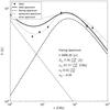 |
Fig. 8 Modeled spectrum for the 2006.20 observations. The dashed-dotted line corresponds to the quiescent spectrum, the dashed line to the flaring spectrum, and the solid black line to the total spectrum. The gray lines indicate the uncertainties in the calculation of the spectrum (for more details see Sect. 5.3). |
Once the spectra are calculated, it is straightforward to obtain the modeled light curves at a given frequency. The comparison between the modeled and the observed 37 GHz light curve is presented in Fig. 9. Although similar plots can be obtained for other frequencies, it is meaningful to select a frequency at which the observed emission is mainly generated by the interaction of the traveling shock with the underlying flow. Moreover, the dense sampling of the 37 GHz observations provided a more complete picture of the evolution of the flaring event. Taking this consideration into account, we picked the 37 GHz light curve as the best possible comparison. The observed data points fall well within the range of modeled light curve. At the beginning of the flare, the 37 GHz flux density was still in its quiet state and therefore the main uncertainty for this time is due to the uncertainties in the quiescent spectrum. The error band presented here corresponds only to the flaring state, which was the dominant contribution to the 37 GHz flux density after 2005.60, leading to broader error bands from this epoch and on.
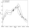 |
Fig. 9 Modeled and observed 37 GHz light curve. The black solid line corresponds to the calculated model and the dashed lines indicate the uncertainties in the calculation of the modeled light curve (for more details see text). |
5.4. Rejected solutions
As already mentioned, the solutions for the spectral fitting were embedded in a 4- or 5-dimensional parameter space. Some of those can be highly degenerate given the small number of data points. When fitting the spectral evolution, a deep study of the parameter space was performed, including all possible combinations of the parameters (i.e., variation of single, pairs and triplets of parameters) and simultaneously fitted stages (one-, two- and three-stage fits). Within this study we found families of solutions with χ2 values similar to the presented final set of parameters, but with unphysical values. After a sanity check, those fits were discarded. The meaningful set of solutions is presented in Table 7 and discussed in Sect. 6.
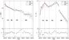 |
Fig. 10 Temporal evolution of the 2006 radio flare in CTA 102 modeled with varying Doppler factor (black solid line) for t > 2006.0 and with the modifications of Björnsson & Aslaksen (2000) for the first two stages (red solid line). Both models fail to describe the 2006 flare (compare to Fig. 7); left: turnover frequency; right: turnover flux density. The lower panels show the residuum for the fits |
5.4.1. The geometrical model
Stevens et al. (1996) found a similar double hump in the νm − Sm plane for 3C 345. They assumed that this behavior could be due to changes of the viewing angle, expressed in a variation of the Doppler factor, D, along the jet. Therefore we used as an alternative to the previous modeling of the second hump in the νm − Sm plane, a purely geometrical approach. Such an approach could easily explain the variation in the observed turnover flux density  while the observed turnover frequency kept a nearly constant value
  . It was assumed that the deviation from the standard shock-in-jet model around 2005.95 was caused by changes in the evolution of the Doppler factor D = Γ-1(1 − βcosϑ)-1 during the final adiabatic loss stage. The remaining parameters were taken from the best fit to the evolution until 2006.0 (first column in Table 7, model C1A1) and only the parameter d was allowed to vary.
The result of our calculations for the different models is presented in Fig. 10 and Table 8. The figure shows the fits separating the different stages observed after 2006.0 (Figs. 4 and 5). We recall that these stages are the increase of the flux density between 2006.0 and 2006.3 and the decrease in flux density and frequency from 2006.3 until 2006.8.
It is obvious that a simple change in the evolution of the Doppler factor, expressed by the exponent d,  , can not explain the observed temporal evolution of the turnover frequency and turnover flux density.
Results of the geometrical model for parameter d.
Spectral parameters for C1A1 using Björnsson & Aslaksen (2000).
5.4.2. Applying the modified COMPTON stage
As mentioned in Sect. 3, Björnsson & Aslaksen (2000) reviewed Marscher & Gear (1985) assumption for the Compton stage and modified the equations for the evolution of the turnover frequency, νm, and the turnover flux density, Sm. We applied this model to the first two stages of the 2006 flare in CTA 102 (Model C1A1), using the expression as in Sect. 3.2 for the time evolution (Eq. (39)) and d = 0. The result of the modeling is shown in Figs. 11, 10 and Table 9.
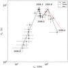 |
Fig. 11 The 2006 radio flare in the turnover frequency-turnover flux density plane. The time labels indicate the time evolution and the temporal position of local and global extrema in the spectral evolution. The black line corresponds to the final model presented in Table 7 (based on Marscher & Gear 1985) and the red one to Table 9 (based on Björnsson & Aslaksen 2000). |
The result of the fitting shows that the approach of Björnsson & Aslaksen (2000) cannot explain the steep rise of the turnover flux density with decreasing turnover frequency in the first stage of the flare (see solid red line in Fig. 11). Following the authors, this could be an indication that inverse Compton scattering is not the dominant energy loss mechanism during the rising stage (Björnsson & Aslaksen 2000). This aspect will be discussed in Sect. 6.
6. Discussion
Our analysis of the strong radio flare observed in CTA 102 around 2006, shows that its behavior until epoch 2006.0, i.e., the first hump in the νm − Sm plane, can be well modeled by a Compton and adiabatic stage within the standard shock-in-jet model (Marscher & Gear 1985) (see Sect. 5.1.1). We found no evidence of a synchrotron stage between the Compton and the adiabatic stages during the first part of the evolution. This behavior was similar to the one found in another prominent blazar 3C 345 (Lobanov & Zensus 1999), where a bright jet component also appeared to proceed from the Compton stage to the adiabatic stage, with the synchrotron stage ruled out by combination of the observed spectral and kinematic evolution of this component. The flare in CTA 102 shows a second hump in the νm − Sm plane (see Fig. 11) after 2006.0, that cannot be explained within this model. The evolution between 2006.0 and 2006.3 seems to follow the predicted evolution of a Compton stage, i.e., increasing turnover flux density and decreasing the turnover frequency. Based on this apparent behavior we applied the equations of the Compton stage to this second hump (see Sect. 5.1.2). After epoch 2006.3, the evolution shows a decrease in both turnover values, which can be interpreted as an adiabatic stage. Thus, we used the appropriate equations for this stage to fit the data points (see Sect. 5.1.3). This approach led to a set of exponents which describe the evolution of the magnetic field, B, the Doppler factor, D, the spectral slope of the electron distribution, s, the normalization coefficient of the relativistic electron distribution, K, and the jet radius, R. The results of our modeling are summarized in Fig. 7. Our hypothesis is that this behavior can be interpreted in terms of the interaction between a traveling shock and a standing shock wave in an over-pressured jet. A pure geometrical model failed to explain the observed behavior (see Sect. 5.4.1). We also tried to fit the evolution of the flare using the modification of the shock-in-jet model by Björnsson & Aslaksen (2000), but this also failed. However, the failure of this model, which takes into account multiple Compton scattering, could have further implications in our understanding of flaring events in AGN jets, as discussed at the end of this section.
The formation of a standing shock can be described in the following way: the unbalance between the jet pressure and the pressure of the ambient medium at the jet nozzle leads to an opening of the jet. Due to the conservation laws of hydrodynamics, this opening results in a decrease of the density, the pressure and the magnetic field intensity in the jet. The finite speed of the sound waves in the jet is responsible for an over-expansion followed by a re-collimation of the jet that gives rise to the formation of a shock. During this collimation process the jet radius decreases and the shock leads to an increase of the pressure, density, and magnetic field intensity. Again, the finite speed of the sound waves is responsible for a over-collimation of the jet. This interplay between over-expansion and over-collimation leads to the picture of a pinching flow, i.e., a continuous change of the width along the jet axis, in contrast to conical jets. The intrinsic physical parameters (pressure, density, and magnetic field) along a pinching jet show a sequence of local maxima and minima (Daly & Marscher 1988; Falle 1991).
Summarizing, an over-pressured jet can be divided into three regions, i) the expansion region, i.e., continuous increase of the jet radius; ii) the collimation region, i.e., decrease of the jet radius and formation of the collimation shock; and iii) the re-expansion region (see Fig. 12). In such a scenario, enhancements of emission can be produced by the interaction between traveling and standing (re-collimation) shocks (Gómez et al. 1997). In the following, the evolution of the travelling shock in these regions is described and our results are put in context.
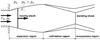 |
Fig. 12 Sketch of an over-pressured jet with indicated characteristic regions (adopted from Daly & Marscher 1988). |
6.1. The expansion region
A relativistic shock propagating through this region accelerates particles at the shock front. These particles travel behind the shock and suffer different energy loss mechanisms, depending on their energy. The resulting evolution of the turnover frequency and turnover flux density is explained by the shock-in-jet model (Marscher & Gear 1985) under certain assumptions.
The parameters derived for the time between 2005.6 and 2006.0 can be associated with this region, including a Compton and an adiabatic stage. The expansion of the jet is parametrized by r = 0.60, which differs from the value expected for a conical jet r = 1. The non-conical behavior could be due to acceleration of the flow (Marscher 1980). This acceleration should be expressed by − r·d > 0 (D ∝ L − rd). However, from our results, this value is negative − r·d = −0.12, but very small, i.e., compatible with no changes in the Doppler factor. Thus, we cannot confirm this point.
For the evolution of the magnetic field with distance we derive a value of b = 1.0, indicating that the magnetic field could be basically toroidal in this region. The injected spectral slope for the relativistic electron distribution s = 2.1 leads to an optically thin spectral index α0 = −0.55. A decrease in the density can be deduced from − r·k = −1.6, which corresponds to the evolution of the normalization coefficient of the relativistic electron distribution, K.
The parameter toff corresponds to the time difference between the onset of the Compton stage and the first detection of the flare. From the value of toff = 0.02 yr together with independently obtained values for the viewing angle, ϑ = 2.6°, and the apparent speed of the VLBI component ejected by the 2006 flare, βapp = 17 c (Jorstad et al. 2005; Fromm et al. 2011), we calculated the displacement between the onset and the detection of the flare to be Δr = 3.5 pc.
6.2. The collimation region
After the recollimation region, at the position of the hypothetical standing shock, the local increase in density, pressure and magnetic field should generate an increase in the emission. The interaction between a travelling and a standing shock would further enhance the emission (Gómez et al. 1997). Furthermore, the standing shock would be dragged downstream by the traveling shock and re-established after a certain time at its initial position (Gómez et al. 1997; Mimica et al. 2009). We compare here our results with this scenario.
Since the evolution of the turnover frequency and turnover flux density between 2006.0 and 2006.3 showed Compton-stage-like behavior, i.e., decreasing turnover frequency and increasing flux density, we used the equations of the Compton stage to derive the possible evolution of the physical parameters (model C2). In this region a slower rate of jet expansion is found (r = 0.35). During this stage, the Doppler factor seems to be constant with distance, − r·d = 0.035. In the context of the hypothetical shock-shock interaction, acceleration of the flow close to the axis is expected down to the discontinuity of the stading shock, where sudden deceleration would occur (see, e.g., Perucho & Martí 2007). Thus, it is difficult to assess whether the Doppler factor should increase or decrease in the whole region.
The magnetic field intensity decreases with an exponent b = 1.35, implying that the geometry of the magnetic field has changed, with contributions of non-toroidal components, but showing no hints of magnetic field enhancement. The parameter s, giving the spectral slope of the relativistic electron distribution changes to s = 2, which gives an optically thin spectral index α0 = −0.5.
The set of parameters derived for this time interval do not reflect the expected physical conditions of a traveling-standing shock interaction, other than a slight flattening of the spectral slope (from possible refreshment of particles). Nevertheless, the shock-shock scenario could hardly be reproduced by a one-dimensional model. Numerical simulations should be performed in order to study this hypothesis in detail. Another possibility is that the reason for the second peak is attached to the injection of a second shock from the basis of the jet. This is not observed, though.
6.3. The re-expansion region
After the re-collimation process, the jet re-expands, i.e., the jet radius increases again. In principle, the position of the re-collimation shock can be regarded as a “new” nozzle from which the fluid emerges. Therefore, when the shock front reaches this region, the expected evolution is, again, that predicted by the shock-in-jet model.
The evolution between 2006.3 and 2006.8 is identified within our hypothesis with the re-expansion region. Thus, the equations for an adiabatic loss stage were applied to the evolution turnover frequency and turnover flux density.
The opening of the jet is clearly apparent at this stage r = 0.90. This opening should produce a decrease in density, which translated into smaller values of the parameter − r·k,  . From the fits, we derive − r·k = −4.2, confirming a decay in the density. The magnetic field falls with b = 1.7, which shows again that the geometry of the field changes from a purely toroidal to a mixed structure with the distance. The values for − r·d = 0.18 reveal an acceleration of the flow, which can naturally arise during the expansion of the jet. The spectral slope of s = 2.4 translates into an optically thin spectral index of α0 = −0.7.
6.4. Spectral slopes and optically thin spectral indices
The variation of the fitted optically thin spectral index, α0,f, (see upper panel in Fig. 6) is an indication of the aging of the relativistic electron distribution due to the different energy loss mechanisms during the evolution of the flare. The model presented by Marscher & Gear (1985) did not include such an aging of the relativistic electron distribution. Despite this restriction, we could model the qualitative behavior of the evolution via the different values obtained for parameter s in the different fitted stages: for the expansion region we obtained α0,m = −0.55, a slightly flatter spectral index for the collimation region α0,m = −0.50 and a steeper value for the re-expansion α0,m = −0.7.
6.5. The influence of the interpolation and the quiescent spectrum
We applied several interpolation steps together with different quiescent spectral parameters to the analysis of the light curves in order to test their influence on the study of the evolution of the peak parameters in the turnover frequency-turnover flux density (νm − Sm) plane. All the tests showed a second hump in the νm − Sm plane. From the tests, the positional shifts (in time of appearance, turnover frequency and turnover flux density) of the second hump were calculated: the hump appeared at t = 2006.30 ± 0.05 yr at a turnover frequency  and turnover flux density
  .
.
These tests proved that the increase of the turnover frequency and turnover flux density around 2006.3 is not an artifact generated by the interpolation and/or the choice of the quiescent spectrum.
6.6. Adiabatic versus non-adiabatic shock
Björnsson & Aslaksen (2000) suggested that the steep slopes in the rising region of the νm − Sm-plane, which is generally identified as the Compton stage in the shock-in-jet model, could not be due to Compton radiation, but to other processes such as isotropization of the electron distribution or even to the non-adiabatic nature of the shock.
The slope we obtained for this time-interval in the νm − Sm plane is too steep to be reproduced by the model presented in Björnsson & Aslaksen (2000) (see Sect. 5.4.2). Thus, the non-adiabatic nature of the first stages of evolution of shocks in extragalactic jets remains an open issue on the basis of our limited data set.
7. Summary and conclusions
In this work we present the analysis of the 2006 flare in CTA 102 in the cm − mm regime. The obtained evolution could be well described, up to a certain point (t < 2006.0), with the standard shock-in-jet model (Marscher & Gear 1985). In order to model the further evolution of the flare we proposed a second Compton-like stage and a second adiabatic stage. We derived the evolution of the physical parameters of the jet and the flare and we performed a parameter space analysis to obtain the uncertainties of the values obtained. From the modeled parameters, together with their uncertainties, the theoretical light curves and spectra were computed. The result was shown to be in fair agreement with the observations.
However, the shock-in-jet model is not able to reproduce the second peak of the double-hump structure found in the evolution of the peak flux – peak frequency plane in a consistent way within our hypothesis of a shock-shock interaction. This is surely due to the complexity of the situation and does not rule out our hypothesis. Numerical simulations will be performed to test it. The goodness of the fit in this region may be due basically to the lack of observational data as compared to the number of parameters implied in the modeling.
Moreover, our results show that some of the basic assumptions of the present models should be reviewed. In particular, we found that the first stage of the studied evolution could be incompatible with an adiabatic behavior if the model of Björnsson & Aslaksen (2000) is correct.
We plan to improve our results by performing a similar analysis to multifrequency VLBI observations. Future work on the spectral evolution of components in jets, especially the interaction between traveling shocks and re-collimation shocks, should include numerical simulations to help to understand this non-linear phenomenon, and improve the strong limitations of the assumptions required by the shock-in-jet and other analytical models. The analysis of multifrequency VLBI observations during the 2006 radio flare in CTA 102 will be presented in Paper II.
Marscher & Gear (1985) included only first order Compton scattering.
Acknowledgments
C.M.F. was supported for this research through a stipend from the International Max Planck Research School (IMPRS) for Astronomy and Astrophysics at the Universities of Bonn and Cologne. Part of this work was supported by the COST Action MP0905 Black Hole in a violent Universe. C.M.F. was supported during his Diploma Thesis by Kölner Gymnasial − und Studienstiftung. C.M.F. thanks the Departament d’Astronomia i Astrofísica of the University València for its hospitality. M.P. acknowledges financial support from the Spanish “Ministerio de Ciencia e Innovación” (MICINN) grants AYA2010-21322-C03-01, AYA2010-21097-C03-01 and CONSOLIDER2007-00050, and from the “Generalitat Valenciana” grant “PROMETEO-2009-103”. M.P. acknowledges support from MICINN through a “Juan de la Cierva” contract. E.R. acknowledges partial support by the Spanish MICINN through grant AYA2009-13036-C02-02. Part of this work was carried out while T.S. was a research fellow of the Alexander von Humboldt Foundation. This work is based on observations with the radio telescope of the university of Michigan, MI, USA, the Metsähovi radio telescope of the university of Helsinki, Finland and Submillimeter Array (SMA) of the Smithsonian Astrophysical Observatory, Cambridge, MA, USA. The operation of UMRAO is made possible by funds from the NSF and from the university of Michigan. The Submillimeter Array is a joint project between the Smithsonian Astrophysical Observatory and the Academia Sinica Institute of Astronomy and Astrophysics and is funded by the Smithsonian Institution and the Academia Sinica. The Metsähovi team acknowledges the support from the Academy of Finland to our observing projects. We thank Maria Massi and Petar Mimica for fruitful discussions and comments.
References
- Abdo, A. A., Ackermann, M., Ajello, M., et al. 2009, ApJS, 183, 46 [NASA ADS] [CrossRef] [Google Scholar]
- Altschuler, D. R., Gurvits, L. I., Alef, W., et al. 1995, A&AS, 114, 197 [NASA ADS] [Google Scholar]
- Bååth, L. B. 1988, The Impact of VLBI on Astrophysics and Geophysics; Proceedings of the 129th IAU Symp., 129, 117 [NASA ADS] [Google Scholar]
- Björnsson, C.-I., & Aslaksen, T. 2000, ApJ, 533, 787 [NASA ADS] [CrossRef] [Google Scholar]
- Daly, R. A., & Marscher, A. P. 1988, ApJ, 334, 539 [NASA ADS] [CrossRef] [Google Scholar]
- Falle, S. A. E. G. 1991, MNRAS, 250, 581 [NASA ADS] [CrossRef] [Google Scholar]
- Fromm, C. M. 2009, High Resolution Studies of AGN, Diploma Thesis, Rheinische Friedrich Wilhelms Universität Bonn [Google Scholar]
- Fromm, C. M., Ros, E., Savolainen, T., et al. 2011, MmSAlt, 82, 65 [NASA ADS] [Google Scholar]
- Gómez, J. L., Martí, J. M. A., Marscher, A. P., Ibáñez, J. M. A., & Alberdi, A. 1997, ApJ, 482, L33 [NASA ADS] [CrossRef] [Google Scholar]
- Harris, D. E., & Roberts, J. A. 1960, PASP, 72, 237 [NASA ADS] [CrossRef] [Google Scholar]
- Hewitt, A., & Burbidge, G. 1989, ApJS, 69, 1 [NASA ADS] [CrossRef] [Google Scholar]
- Hovatta, T., Valtaoja, E., Tornikoski, M., & Lähteenmäki, A. 2009, A&A, 494, 527 [NASA ADS] [CrossRef] [EDP Sciences] [Google Scholar]
- Jorstad, S., Marscher, A., Stevens, J., et al. 2005, Future Directions in High Resolution Astronomy, The 10th Anniversary of the VLBA, 340, 183 [Google Scholar]
- Kardashev, N. S. 1964, Soviet Ast., 8, 217 [Google Scholar]
- Königl, A. 1981, ApJ, 243, 700 [NASA ADS] [CrossRef] [Google Scholar]
- Lampton, M., Margon, B., & Bowyer, S. 1976, ApJ, 208, 177 [NASA ADS] [CrossRef] [Google Scholar]
- Lind, K. R., & Blandford, R. D. 1985, ApJ, 295, 358 [NASA ADS] [CrossRef] [Google Scholar]
- Lister, M. L., Aller, H. D., Aller, M. F., et al. 2009a, AJ, 137, 3718 [NASA ADS] [CrossRef] [Google Scholar]
- Lister, M. L., Cohen, M. H., Homan, D. C., et al. 2009b, AJ, 138, 1874 [NASA ADS] [CrossRef] [Google Scholar]
- Lobanov, A. P., & Zensus, J. A. 1999, ApJ, 521, 509 [NASA ADS] [CrossRef] [Google Scholar]
- Marscher, A. P. 1980, ApJ, 235, 386 [NASA ADS] [CrossRef] [Google Scholar]
- Marscher, A. P. 1990, in Parsec-Scale Radio Jets, ed. J. A. Zensus, & T. J. Pearson (Cambridge: Cambridge Univ. Press), 236 [Google Scholar]
- Marscher, A. P., & Gear, W. K. 1985, ApJ, 298, 114 [NASA ADS] [CrossRef] [Google Scholar]
- Mimica, P., Aloy, M.-A., Agudo, I., et al. 2009, ApJ, 696, 1142 [NASA ADS] [CrossRef] [Google Scholar]
- Nolan, P. L., Bertsch, D. L., Fichtel, C. E., et al. 1993, ApJ, 414, 82 [NASA ADS] [CrossRef] [Google Scholar]
- Pacholczyk, A. G. 1970, Radio astrophysics. Nonthermal processes in galactic and extragalactic sources (San Francisco: Freeman) [Google Scholar]
- Perucho, M., & Martí, J. M. 2007, MNRAS, 382, 526 [NASA ADS] [CrossRef] [Google Scholar]
- Pica, A. J., Smith, A. G., Webb, J. R., et al. 1988, AJ, 96, 1215 [NASA ADS] [CrossRef] [Google Scholar]
- Rantakyrö, F. T., Wiik, K., Tornikoski, M., Valtaoja, E., & Bååth, L. B. 2003, A&A, 405, 473 [NASA ADS] [CrossRef] [EDP Sciences] [Google Scholar]
- Savolainen, T., Wiik, K., Valtaoja, E., Jorstad, S. G., & Marscher, A. P. 2002, A&A, 394, 851 [NASA ADS] [CrossRef] [EDP Sciences] [Google Scholar]
- Sholomitskii, G. B. 1965, Soviet Ast., 9, 516 [NASA ADS] [Google Scholar]
- Spencer, R. E., McDowell, J. C., Charlesworth, M., et al. 1989, MNRAS, 240, 657 [NASA ADS] [CrossRef] [Google Scholar]
- Stevens, J. A., Litchfield, S. J., Robson, E. I., et al. 1996, ApJ, 466, 158 [NASA ADS] [CrossRef] [Google Scholar]
- Tornikoski, M., Terasranta, H., Balonek, T. J., & Beckerman, E. 1999, BL Lac Phenomenon, Takalo, L.O. & Sillanpää, A. (eds.), ASP Conf. Ser. 159 (San Francisco, CA: Astronomical Society of the Pacific), 307 [Google Scholar]
- Türler, M., Courvoisier, T. J.-L., & Paltani, S. 2000, A&A, 361, 850 [NASA ADS] [Google Scholar]
- Véron-Cetty, M.-P., & Véron, P. 2003, A&A, 412, 399 [NASA ADS] [CrossRef] [EDP Sciences] [Google Scholar]
- Wehrle, A. E., & Cohen, M. 1989, ApJ, 346, L69 [NASA ADS] [CrossRef] [Google Scholar]
- Zensus, J. A., Ros, E., Kellermann, K. I., et al. 2002, AJ, 124, 662 [NASA ADS] [CrossRef] [Google Scholar]
All Tables
Average time sampling and average flux density uncertainties for the used light curves.
Spectral parameters (expected values) and corresponding uncertainties from the Monte-Carlo simulation.
Range for spectral parameters allowed to vary in the fits to the observed spectrum for all stages.
Best fit values for spectral evolution modeling of the 2006 radio flare in CTA 102, parameters b, d, s, kr and t.
All Figures
|
Fig. 1 Radio-mm light curves for CTA 102, centered around the 2006 radio flare. |
| In the text | |
|
Fig. 2 Archival low frequency light curves for CTA 102. See insert plot for the absolute quiescent state. |
| In the text | |
|
Fig. 3 Result of the spectral fitting to the 2006.20 data. The dashed-dotted line corresponds to the quiescent spectrum, the dashed line to the flaring spectrum, and the solid black line to the total spectrum. The values presented indicate the spectral turnover of the flaring spectrum. |
| In the text | |
|
Fig. 4 The 2006 radio flare in the turnover frequency-turnover flux density plane. The time labels indicate the time evolution and the temporal position of local and global extrema in the spectral evolution. |
| In the text | |
|
Fig. 5 Temporal evolution of the 2006 radio flare: top turnover frequency and bottom turnover flux density. The dashed vertical lines correspond to the time labels in Fig. 4 and indicate the extrema in the evolution. |
| In the text | |
|
Fig. 6 Temporal evolution of the optically thin (α0, top) and thick (αt, bottom) spectral indices for 2006 radio flare. The dashed vertical lines corresponds to the time labels in Fig. 4 and indicate the extrema in the evolution. |
| In the text | |
|
Fig. 7 Temporal spectral evolution of the 2006 radio flare in CTA 102 left: turnover frequency; right: turnover flux density. The lower panels show the residuum for the fits |
| In the text | |
|
Fig. 8 Modeled spectrum for the 2006.20 observations. The dashed-dotted line corresponds to the quiescent spectrum, the dashed line to the flaring spectrum, and the solid black line to the total spectrum. The gray lines indicate the uncertainties in the calculation of the spectrum (for more details see Sect. 5.3). |
| In the text | |
|
Fig. 9 Modeled and observed 37 GHz light curve. The black solid line corresponds to the calculated model and the dashed lines indicate the uncertainties in the calculation of the modeled light curve (for more details see text). |
| In the text | |
|
Fig. 10 Temporal evolution of the 2006 radio flare in CTA 102 modeled with varying Doppler factor (black solid line) for t > 2006.0 and with the modifications of Björnsson & Aslaksen (2000) for the first two stages (red solid line). Both models fail to describe the 2006 flare (compare to Fig. 7); left: turnover frequency; right: turnover flux density. The lower panels show the residuum for the fits |
| In the text | |
|
Fig. 11 The 2006 radio flare in the turnover frequency-turnover flux density plane. The time labels indicate the time evolution and the temporal position of local and global extrema in the spectral evolution. The black line corresponds to the final model presented in Table 7 (based on Marscher & Gear 1985) and the red one to Table 9 (based on Björnsson & Aslaksen 2000). |
| In the text | |
|
Fig. 12 Sketch of an over-pressured jet with indicated characteristic regions (adopted from Daly & Marscher 1988). |
| In the text | |
Current usage metrics show cumulative count of Article Views (full-text article views including HTML views, PDF and ePub downloads, according to the available data) and Abstracts Views on Vision4Press platform.
Data correspond to usage on the plateform after 2015. The current usage metrics is available 48-96 hours after online publication and is updated daily on week days.
Initial download of the metrics may take a while.