| Issue |
A&A
Volume 531, July 2011
|
|
|---|---|---|
| Article Number | A103 | |
| Number of page(s) | 9 | |
| Section | Atomic, molecular, and nuclear data | |
| DOI | https://doi.org/10.1051/0004-6361/201016216 | |
| Published online | 21 June 2011 | |
Collisional excitation of sulfur dioxide in cold molecular clouds*
1
CAB. INTA-CSIC. Department of Astrophysics. Crta Torrejón km 4. Torrejón de Ardoz, Madrid, Spain
e-mail: This email address is being protected from spambots. You need JavaScript enabled to view it.
2
LERMA and UMR 8112 of CNRS, Observatoire de Paris-Meudon, 92195 Meudon Cedex, France
e-mail: This email address is being protected from spambots. You need JavaScript enabled to view it.
3
Laboratoire d’Astrophysique de Grenoble, UMR 5571-CNRS, Université Joseph Fourier, Grenoble, France
e-mail: This email address is being protected from spambots. You need JavaScript enabled to view it.
Received: 26 November 2010
Accepted: 5 April 2011
Abstract
We present collisional rate coefficients for SO2 with ortho and para molecular hydrogen for the physical conditions prevailing in dark molecular clouds. Rate coefficients for the first 31 rotational levels of this species (energies up to 55 K) and for temperatures between 5 and 30 K are provided. We have found that these rate coefficients are about ten times more than those previously computed for SO2 with helium. We calculated the expected emission of the centimeter wavelength lines of SO2. We find that the transition connecting the metastable 202 level with the 111 one is in absorption against the cosmic background for a wide range of densities. The 404−313 line is found to be inverted for densities below a few 104 cm-3. We observed the 111−202 transition with the 100 m Green Bank Telescope towards some dark clouds. The line is observed, as expected, in absorption and provides an abundance of SO2 in these objects of a few 10-10. The potential use of millimeter lines of SO2 as tracers of the physical conditions of dark clouds is discussed.
Key words: molecular processes / ISM: molecules / ISM: abundances
Tables 5 and 6 are only available at the CDS via anonymous ftp to cdsarc.u-strasbg.fr (130.79.128.5) or via http://cdsarc.u-strasbg.fr/viz-bin/qcat?J/A+A/531/A103
© ESO, 2011
1. Introduction
The observation of molecular emission at millimeter and infrared wavelengths, supplemented by careful and detailed modeling, is a powerful tool for investigating the physical and chemical conditions of astrophysical objects. Since the detection of sulfur dioxide, SO2, by Snyder et al. (1975), this molecule has been found to be very abundant (relative to H2) in warm molecular clouds (Schilke et al. 2001; Schloerb et al. 1983). It has also been observed towards cold dark clouds with an abundance of a few 10-9 (Irvine et al. 1983; Dickens et al. 2000). Interpretation of the data requires a precise knowledge of the collisional rates of the molecule under study and the main colliders in the cloud, i.e., molecular hydrogen and helium. Green (1995) has computed these rate coefficients1 for the system SO2-He for temperatures between 25−125 K for the first 50 rotational levels of this molecule (i.e., for levels with energies below 90 K). These rates are useful for clouds with temperatures around 25−40 K. However, for warm molecular clouds in which lines involve energy levels of several hundred K, or in O-rich evolved stars that show lines with levels of more than one thousand Kelvin, adequate radiative transfer models cannot be carried out owing to the lack of collisional rates at these high temperatures. Moreover, for dark clouds it will be extremely difficult to extrapolate the rates from 25 K to 10 K, which is the typical temperature of these objects, as many resonances occur at low energies and may make a strong contribution to collisional rates when the temperature decreases.
SO2 is one of the molecular species that is being observed with the Herschel Space Observatory in the submillimeter and far-infrared domains thereby increasing the number of transitions and also increasing the energies of observed rotational levels. The new generation of receivers for ground-based telescopes will permit sensitive line surveys to be carried out in dark clouds in the centimeter and millimeter domains. It would be a pity if all these observational efforts do not provide outstanding science because of the lack of collisional rates. In this paper, we provide collisional rates for temperatures from 5 to 30 K for the first 31 levels of SO2. In a subsequent paper, we will provide calculations for high temperatures and for a large number of rotational levels.
Considering the sensitivity of the radiative transfer models to the collisional rate coefficients, it is very important to provide accurate values for these coefficients. Thanks to recent progress in quantum chemistry calculations of the potential energy interaction between the two collision partners, scattering calculations based on the quantum close coupling (CC) method can provide the best accuracy to date, a few percent (Lique et al. 2010).
The methods and the results for the collisional rates are described in Sect. 2. In Sect. 3 we discuss the scope of the new collisional rates and predict the expected emission of several lines of SO2 in dark clouds. In particular, we show that the line 111 − 202 could be in absorption against the cosmic background and that the 404−313 line could be a strong maser in dark clouds.
2. Inelastic cross sections and rates for excitation of SO2 by para and ortho H2
2.1. Potential energy surface and general procedure
All calculations presented below were performed with rigid molecules using the expansion of the 5D-PES described in Spielfiedel et al. (2009) where full details can be found. We used the conventions of Phillips et al. (1996) in defining the SO2-H2 intermolecular potential in the body-fixed frame. The SO2 molecule lies in the xz plane with the symmetry axis along z. The rigid body PES involves five coordinates: the collision coordinate, i.e. the vector from SO2 center of mass to H2 center of mass, described by the spherical polar coordinates (R,θ,φ), and the (θ′,φ′) angles giving the H2 orientation relative to the SO2 molecule in the body-fixed system.
Following the strategy developed for the H2O-H2 system (Valiron et al. 2008), the PES was calculated at the CCSD(T) level using a three-step procedure with basis sets of increasing accuracy and a complete basis set (CBS) extrapolation. Extensive calculations of a reference PES were performed for 49 intermolecular distances and 8074 sets of angles for each distance using the aVDZ basis of Woon et al. (1994) and bond functions from William et al. (1995). Corrections, including CBS extrapolation, were performed to obtain the final intermolecular potential. The global minimum was found to be Vmin = −192.723758 cm-1 for R = 6.147979 Bohr, θ = 91.721778°, φ = 90.0°, θ′ = 90.0° and φ′ = 0°. Seven secondary minima were also found. The angular expansion of the PES was obtained from the final very accurate set as a least square fit of the ab initio values for each of 49 intermolecular distances, leading to 129 angular functions that are specifically adapted to quantum calculations. The selection was found to reproduce the ab initio values within 1 cm-1 for distances R greater than 6.5 a0. This result indicates the high quality of the angular fit in the long-range and van der Waals minimum regions of the interaction.
Close coupling calculations were performed with the mixed MPI and OpenMP2 extension of the MOLSCAT V14 package (Hutson & Green 1994). The asymmetric top wave functions of 32SO2 were obtained from the rotational constants and distortion constants given by Lovas (1978) and evaluated in the same coordinate system as was used to describe the PES. The rotational constants about the x, y, and z axes are 2.027354, 0.29353, and 0.344170 cm-1. The adopted centrifugal distortion constants (for a non-rigid asymmetric rotor) for SO2 in its vibrational ground state are −7.2235 × 10⁻⁷, 3.3550 × 10⁻⁶, and 1.0267 × 10⁻⁵ cm-1. For 32SO2-H2 the reduced mass is 1.9540708 amu. The symmetry axis (z-axis) corresponds, in standard spectroscopic notation, to the b-axis. The nuclear spin statistics for the identical oxygen nuclei with spin 0 allow only asymmetric top levels, jKaKc, with Ka, Kc either ee or oo, where e/o indicates even/odd integer values (Green 1995). The calculated energies of the lowest 31 rotational levels of SO2 are compared in Table 1 to the values given in the JPL catalog (Pickett et al. 1998).
SO2 calculated energy levels (in cm-1) compared to values deduced from the JPL molecular spectroscopy catalog in Pickett et al. (1998).
The calculations were carried out using the hybrid log-derivative Airy propagator of Alexander & Manolopoulos (1987). The various propagation parameters were tested to obtain convergence for the lowest 31 levels and for collision energies up to 150 cm-1. Typically the minimum and the maximum integration range was Rmin = 5 and Rmax = 40 bohr. The Airy propagation starts from R = 20 bohr with an accuracy parameter taken as 0.0003. We increased the MOLSCAT’s parameter STEPS from 10 at the highest energies (≥100 cm-1) up to 70 at the lowest energy in order to properly describe the details of the radial function. Our calculations provide state-to-state collisional rate coefficients for the 31 lowest SO2 levels, 72 levels were included in the basis set to obtain convergence better than 5% on the collisional cross sections. Two calculations for excitation of SO2 by para-H2 were performed, the first one was restricted to H2 (jH2 = j2 = 0) and the second one includes in addition the closed j2 = 2 channel. For ortho-H2, the j2 = 3 level of H2 was considered unnecessary at the investigated energies and only the j2 = 1 level was included.
The energy grid, detailed in Table 2 (with E = Ec + Erot(SO2) where Ec is the kinetic energy), was adjusted to reproduce all the details of the resonances as they are essential to calculate the rates with high confidence. Due to the increasingly large computer time and memory ressources needed for the calculations, extension of full close-coupling calculations to higher energies than 150 cm-1 is not realistic. So we adopt an extrapolation procedure for energies from 150 cm-1 up to 300 cm-1 in order to obtain fully converged rate coefficients for temperatures up to 30 K. This extrapolation assumes constant values for the cross sections from the last calculated value (150 cm-1). Several controls of this approximation were performed, including evaluation of the contribution of the extrapolated part of the cross sections as well as check of the detailed balance between upwards and downwards rates. At low temperatures, the effect of this extrapolation was found to be negligible and less than one percent at 30 K.
Energy grid of the quantum MOLSCAT cross section calculations.
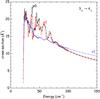 |
Fig. 1 Cross section for excitation by para and ortho-H2 for the 331 → 431 transition as a function of the energy E = Ec + Erot(SO2). Black curve: para-H2(j2 = 0); red curve para-H2 = (j2 = 0,2); blue curve: ortho-H2(j2 = 1). |
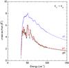 |
Fig. 2 Cross section for excitation by para and ortho-H2 for the 431 → 440 transition as a function of the energy E = Ec + Erot(SO2). Black curve: para-H2(j2 = 0); red curve para-H2 = (j2 = 0,2); blue curve: ortho-H2(j2 = 1). |
Figures 1 and 2 show cross sections for excitation of SO2 by para-H2(j2 = 0), para-H2(j2 = 0,2) and ortho-H2(j2 = 1) for transitions 331 → 431 and 431 → 440. These figures show that cross-sections for para-H2(j2 = 0,2) and (j2 = 0) are almost identical. In particular, these cross-sections display many resonances with similar amplitudes and only a very small shift for some of them. Away from the resonance region, the cross sections vary smoothly with energy. The very small contribution of the H2(j2 = 2) rotational level could be attributed to the high energy of the corresponding closed channels compared to the collisional energy and features of the PES (Spielfiedel et al. 2009).
The situation is different when we compare excitation cross-sections by para and ortho-H2. The cross sections differ both by their amplitudes and by the behavior of the resonances, which are much less pronounced for collisions involving ortho-H2. The weaker impact of resonances on collisions with ortho-H2 was also found in H2O-H2 (Grosjean et al. 2003) and HC3N-H2 (Wernli et al. 2007a,b) collisions. These differences between collisions with para and ortho-H2 could come from the contribution of additional coupling terms (in particular to the dipole-quadrupole term) absent in collisions with para-H2.
Rate coefficients (in cm3 s-1) for the rotational deexcitation of SO2 by collisions with He (Green 1995, scaled), para-H2 (j2 = 0), para-H2 (j2 = 0,2), ortho-H2 (j2 = 1) at T = 25 Ka.
2.2. Para and ortho H2 rates
In the considered energy range, H2 is always in states j2 = 0 and j2 = 1 for para and ortho H2, respectively, so we drop in the following the j2 index. The state-to-state rotational inelastic rates are the Boltzmann thermal average at temperature T of state-to-state inelastic cross sections:  (1)where k is the Boltzmann constant, Ec the kinetic energy, and β = jKa,Kc. Rate coefficients obey the detailed balance relation:
 ![Mathematical equation: \begin{equation} R(\beta' \rightarrow \beta) = \frac{(2j+1)}{(2j'+1)} \textrm {exp} \left[\frac{E_{\beta' } -E_{\beta}}{kT} \right] \; R(\beta \rightarrow \beta'). \label{balance} \end{equation}](/articles/aa/full_html/2011/07/aa16216-10/aa16216-10-eq121.png) (2)We compare in Table 3 a sample of the present collisional rates at 25 K with those of Green (1995). It should be noted that the He rates of Green (1995) have been scaled by the reduced mass ratio of (μSO2 − H2/μSO2 − He)1/2 = 1.39. We first note significant discrepancies between the present rates and the scaled He-rates, even for collisions with para-H2(j = 0). Differences do not vary uniformly with transitions and are found to exceed a factor of ten in some cases. These discrepancies are expected because the rates were computed by Green within the IOS scattering approach based on a coarse electron-gas approximation used for the PES. However, we point out that similar trends for He/H2 have been found for other systems such as SO (Lique et al. 2007), SiS (Lique et al. 2008), HC3N (Wernli et al. 2007a,b), and H2CO (Troscompt et al. 2009), even though the PES’s and the cross sections were computed with the same accuracy. For all these systems, the potential well for interaction with H2 is deeper by a factor of about two than the one found for interaction with He, leading to larger cross sections and rates for collisions with H2. Moreover, preliminary rate coefficients obtained in the IOS approximation with the same SO2-H2 PES as in the present calculations are systematically twice/three times less than the CC results. All these factors contribute to the large underestimation of the scaled He-rates of Green for collisions with H2.
(2)We compare in Table 3 a sample of the present collisional rates at 25 K with those of Green (1995). It should be noted that the He rates of Green (1995) have been scaled by the reduced mass ratio of (μSO2 − H2/μSO2 − He)1/2 = 1.39. We first note significant discrepancies between the present rates and the scaled He-rates, even for collisions with para-H2(j = 0). Differences do not vary uniformly with transitions and are found to exceed a factor of ten in some cases. These discrepancies are expected because the rates were computed by Green within the IOS scattering approach based on a coarse electron-gas approximation used for the PES. However, we point out that similar trends for He/H2 have been found for other systems such as SO (Lique et al. 2007), SiS (Lique et al. 2008), HC3N (Wernli et al. 2007a,b), and H2CO (Troscompt et al. 2009), even though the PES’s and the cross sections were computed with the same accuracy. For all these systems, the potential well for interaction with H2 is deeper by a factor of about two than the one found for interaction with He, leading to larger cross sections and rates for collisions with H2. Moreover, preliminary rate coefficients obtained in the IOS approximation with the same SO2-H2 PES as in the present calculations are systematically twice/three times less than the CC results. All these factors contribute to the large underestimation of the scaled He-rates of Green for collisions with H2.
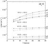 |
Fig. 3 Temperature variation of the de-excitation rate coefficient for transitions with ΔKa = 0. p2 and o1 refer to para and ortho-H2 rate coefficients. |
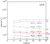 |
Fig. 4 Temperature variation of the de-excitation rate coefficient for transitions with ΔJ = 0. p2 and o1 refer to para and ortho-H2 rate coefficients. |
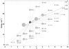 |
Fig. 5 SO2 rotational levels connected to the initial one (431), denoted by a black diamond. Those marked by a gray disk have a para-H2 collisonal excitation or deexcitation rate above the threshold > 10-12 cm3 s-1, with the area of each gray disk proportional to the rate. Crosses correspond to rates below the threshold. |
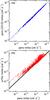 |
Fig. 6 De-excitation rate coefficients of SO2 in collision with para-H2(j2 = 0) as function of rate coefficients with para-H2(j2 = 0,2). The black line indicates equal rates. |
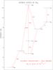 |
Fig. 7 Rotational levels of SO2 with energies below 13 K. Allowed radiative transitions are indicated by red arrows. The numbers indicate the corresponding Einstein coefficients for spontaneous emission in units of 10-8 s-1. |
Figures 3 and 4 display the temperature variation of the para and ortho-H2 rate coefficients for a selection of ΔKa = 0 (Fig. 3) and ΔJ = 0 (Fig. 4) transitions. The following trends are found: the temperature dependence is weak within factor two to three for both para and ortho-H2 collisions. There is no exact selection rule, but the rates decrease for increasing |ΔJ| and |ΔKa|. This propensity is pointed out in Fig. 5, which presents the excitation/deexcitation rates at 25 K for collisions with para-H2 from level JKaKc = 431. One can observe that the most important rates are those that connect levels with |ΔKa| = 0. This trend may be explained by the difficulty of reorienting the angular momentum vector with respect to the a-axis.
Figure 6 compares the de-excitation rate coefficients at 25 K for collisions of SO2 with para-H2(j2 = 0) and ortho-H2 with rate coefficients for collisions with para-H2(j2 = 0,2). It is seen that including of H2(j2) = 2 has a negligible contribution to para-H2 rate coefficients, and that both sets of rates agree within a few percent. Rate coefficients with ortho and para-H2 vary strongly with the transition, with a factor of about two on average, the largest rate coefficients being mainly the rates for collisions with ortho-H2. The latter effect reflects the importance of the H2 quadrupole and in particular the dipole-quadrupole interaction, which does not contribute to collisions with para-H2(j2 = 0).
All rates among the 31 first rotational levels are provided as online material for a temperature range 5 K ≤ T ≤ 30 K (Tables 5 and 6). They will be made available in the LAMDA3 and BASECOL4 databases.
3. SO2 line absorption and maser emission in dark clouds
3.1. Centimeter wavelength transitions
SO2 was detected in interstellar space in the early years of millimeter radioastronomy (Snyder et al. 1975). To our knowledge, all studies of interstellar and circumstellar clouds using SO2 have been performed in the millimeter and submillimeter domains, i.e., by observing rotational transitions involving high energy levels. However, as a heavy species, SO2 has several transitions in the centimeter domain arising from low-lying levels (see Fig. 7). The structure of these levels makes it certain that SO2 should show strong excitation effects in cold dark clouds, that have so far not been analyzed.
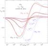 |
Fig. 8 Predicted brightness temperature for the 111 − 202 line of SO2 at 12.256 GHz for different sets of collisional rates. The assumed kinetic temperature and Δv= are 10 K and 1 km s-1, respectively. Black(thin)/red(thick) lines correspond to the excitation of the molecule by o-H2/p-H2 using the collisional rates calculated in this work. Blue(dashed) lines correspond to the predicted intensity when the scaled He-rates of Green (1995) are used. Column densities are indicated and correspond to 3 × 10¹⁴, 1014, 3 × 10¹³, and 1013 cm-2. |
Owing to the C2v symmetry of the molecule, the first excited rotational level, 202 at 2.75 K, is not radiatively connected to the ground level, 000. Consequently, 202 has to be considered as a metastable level. Under non-LTE conditions, e.g. for the physical conditions of dark clouds, it will be overpopulated with respect to the closest level, the 111, at 3.34 K which is radiatively connected to the ground level. Hence, the rotational transition 111−202 at 12 256.583 MHz could be in absorption against the cosmic microwave background for a considerably wide range of densities and temperatures. The Einstein coefficient for the transition 111−000 is (3.5 × 10⁻⁶ s-1), so that high volume densities will be required in order to thermalize the lowest energy levels of SO2, including the metastable one 202.
A second group of rotational levels, 413, 404 and 313 around 12, 9.1, and 7.7 K, respectively, will also show peculiar excitation conditions. The 413 level will radiatively decay towards the 404 one (only possible transition arising from the 413 level; its Einstein coefficient is 3 × 10⁻⁶ s-1), which will slowly decay towards the 313 level. The latter will decay very fast towards the metastable level 202 (see the Einstein coefficients in Fig. 7). The consequence is that the 404 and 313 levels could be inverted; i.e., the transition 404−313 at 29 321.331 MHz could be maser in nature. Although these effects mainly come from the structure of the energy levels and the Einstein coefficients of the rotational transitions, collisions of SO2 with H2 will play an important role in quenching the maser and the absorption lines for some critical densities. In order to quantify these effects, we performed LVG excitation calculations using our new, state of the art, collisional rates for para and ortho H2. The results of our excitation calculations are shown in Figs. 8 and 9 for a kinetic temperature of 10 K and indicate that our qualitative analysis was correct: the 111 − 202 transition will be in absorption and the 404−313 will be maser for a wide range value of volume densities, temperatures, and abundances. For comparison purposes, the results obtained using the collisional rates calculated by Green (1995) for the SO2-He system, scaled by the factor 1.39, are also shown in Figs. 8 and 9. While rotational excitation by ortho and para molecular hydrogen produce similar results, collisions with helium using the rates of Green (1995), corrected by a factor 1.39 to take the different reduced mass of SO2/He and SO2/H2 into account, produces a shift of the curves to higher densities (a factor 10). As discussed in previous sections, this effect is due to the higher SO2-(o/p)-H2 collisional rates (one order of magnitude) than those of the SO2-He system. This effect has been found for all rotational transitions of SO2 arising from the 31 energy levels considered in this paper (see below). This large difference in density between molecular hydrogen and helium rates has deep implications for determining SO2 abundances in cold and warm molecular clouds. The new rates indicate that SO2 rotational levels will be thermalized for densities 10−20 times lower than those predicted from Green’s rates. As a result, SO2 seems more easily thermalized than previously thought. As a consequence, the derived column densities (and abundances) in previous works are probably too high.
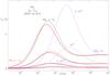 |
Fig. 9 Predicted brightness temperature for the 404−313 line of SO2 at 29.321 GHz for different sets of collisional rates. The assumed kinetic temperature and Δv= are 10 K and 1 km s-1, respectively. Black(thin)/red(thick) lines correspond to the excitation of the molecule by o-H2/p-H2 using the collisional rates calculated in this work. Blue dotted lines correspond to the predicted intensity when the rates of Green (1995) for the SO2-He system are used. Column densities are indicated and correspond to 3 × 10¹⁴, 1014, 3 × 10¹³, and 1013 cm-2. |
Our calculations indicate that, for a density of 3 × 103 cm-3, a kinetic temperature of 10 K (rates for SO2-He have been extrapolated down to 10 K using a square root dependence on the temperature), a linewidth of 1 km s-1, and a column density above 3 × 1012 cm-2 (which could correspond to an abundance of 3 × 10⁻¹⁰ for a cloud of 10 mag of visual absorption), the maser line will have an intensity higher than 0.07 K. The SO2 abundances derived in dark clouds (Irvine et al. 1983; Dickens et al. 2000) range from 2 to 6 × 10⁻⁹, so the 404−313 line could have brightness temperatures above 3 K in most cases. Moreover, the maser line will be the strongest transition of SO2 in cold dark clouds. This is an important issue because the millimeter lines of this species (Snyder et al. 1975; Irvine et al. 1983) are rather weak and have only been observed towards a few selected dense cold cores. Finally, for the range of abundances found for SO2 in dark clouds, the 111−202 absorption line will be as strong as − 0.5 K for these volume densities. Even for column densities as low as 3 × 1012 cm-2, the absorption that could be observed in this line against the cosmic background will be ≃−0.02 K.
We checked that the absorption and masering effects do not depend on the selected temperature within the range of validity of our collisional rates, 5 − 30 K. In particular, we have verified that the factor 10 in density between our collisional rates and those of Green is found not only for 10 K but also for 25 K, the lowest temperature of Green’s calculations (i.e., this factor 10 is not produced by the selected square root extrapolation of Green’s rates from 25 K to 10 K).
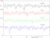 |
Fig. 10 Raw data for the 111 − 202 line of SO2 obtained towards four dark clouds. Although the data suffer from a high-frequency ripple plus spurious features produced by human-made interferences, the absorption features appear clearly in three of them, TMC1, L1527, and L1489. Processed data are shown in Fig. 11. |
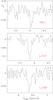 |
Fig. 11 Observed 111−202 line profile towards TMC1, L1527 and L1489. The raw data without any processing are shown in Fig. 10. The x-axis corresponds to LSR velocity and the y-axis corresponds to the observed antenna temperature. |
3.2. Observation of absorption of SO2 against the cosmic background
In spite of their potential for tracing the physical conditions of cold clouds, none of these lines have ever been observed in dark clouds. The 111−202 line is particularly interesting because the new collisional rates indicate that the line will move from absorption to emission for n(H2) > 104 cm-3. The absorption line will therefore be a good tracer of the physical properties of the low-density envelopes of dense cores. Moreover, this line could be used to trace the chemistry of sulfur-bearing molecules in low-density regions (CS, SO, and the millimeter lines of SO2 require high n(H2) values to produce detectable emission). The maser 404−313 line will also be particularly interesting for this purpose.
To check our predictions, we observed four dark clouds in 2009 with the GBT telescope at the frequency of the 111−202 line (12.256 GHz). The selected clouds are TMC1 (α2000 = 04h41m45.9s, δ2000 = 25°41′26.8′′), L1527 (α2000 = 04h39m53.0s, δ2000 = 25°45′0.0′′), L1544 (α2000 = 05h04m18.1s, δ2000 = 25°11′7.9′′), and L1489 (α2000 = 04h04m47.5s, δ2000 = 26°19′42.1′′). Abundant observational data, in several molecular species, is available in the literature for these clouds (Cernicharo & Guélin 1987; Cernicharo et al. 1984; Daniel et al. 2007; Duvert et al. 1986; Fuller et al. 1996; Hogerheijde et al. 1997; Hogerheijde 2001; Myers et al. 1995; Ohashi et al. 1997; Takakuwa et al. 2000; Brinch et al. 2007). Except for TMC1 for which the position corresponds to the cyanopolyyne peak, the selected pointing positions for the other sources correspond to the envelope surrounding the dense cores. As indicated by the calculations shown in Fig. 8, the expected absorption will be weak, will even turn into emission, for densities higher than 104 cm-3.
The observations were done in position-switching mode. At the observing frequency the half power beamwidth of the telescope is 67′′. The spectral resolution was 0.0187 km s-1. The raw data are shown in Fig. 10 without any signal processing except the removal of a degree one baseline. These observations were rather delicate as many human-made spurious signals affected the data despite the protection measurements taken for this site. In addition to the spurious features we also found ripples at different frequencies that were removed by using the GILDAS package. Only a small window around the expected velocity of the clouds, but with enough channels, was finally analyzed for each cloud. The final reduced data are shown in Fig. 11. In spite of the problems found the observations, absorption was observed towards TMC1, L1527, and L1489 at the local standard of rest (LSR) velocity of these clouds. Towards L1544 we obtained only a 3σ upper limit of 0.06 K. Figure 11 shows the observed spectra towards TMC1, L1527, and L1489.
The absorption towards TMC1 peaks at 6.04 km s-1 with a linewidth of 0.09 km s-1 and an intensity of − 0.077 K (Fig. 11 top panel). This cloud is known to show multiple velocity components (Cernicharo et al. 1984; Cernicharo & Guélin 1987; Lique et al. 2006). Figure 11 shows a second possible absorption (3σ) at 5.52 km s-1 with a linewidth of 0.1 km s-1 and an intensity of − 0.038 K. Another sulfur-bearing molecule, SO, has been observed towards this source by Lique et al. (2006), who detected two velocity components at 5.6 and 6.0 km s-1. The agreement in velocity between the SO2 absorption and the emission found in several lines of SO by Lique et al. (2006) is very good. It suggests that the SO2 absorption arises from the same clouds that emit in the SO lines. Lique et al. (2006) have modeled the gas at 6.0 km s-1 with a core of density of 2 × 104 cm-3 surrounded by a low-density envelope of 6 × 103 cm-3 and TK = 10 K for both components. If the observed absorption is arising from the high-density gas, then N(SO2) ≃ 5 × 1012 cm-2. For the assumed volume density the excitation temperature of the 111 − 202 transition is close to 2.7 K, i.e., the turnover density between absorption and emission for this line (see Fig. 8). However, if the absorption is arising from the low-density envelope, then N(SO2) ≃ 1.2 × 1012 cm-2, so the abundance of SO2 is ≃ 2 × 10⁻¹⁰ (for Av = 5 mag in the envelope), i.e., two orders of magnitude below that of SO (Lique et al. 2006). The 5.5 km s-1 cloud was modeled by Lique et al. (2006) with a single density of 8 × 103 cm-3. For this component the derived SO2 column density is 6 × 1011 cm-2.
Towards L1527 we selected a position that corresponds to the envelope of the cloud (Δα = +3′, Δδ = 3.5′ with respect HCL2-A Cernicharo et al. 1984; or Δα ≃ +2′, Δδ ≃ =7′ from TMC1-ATakakuwa et al. 2000). It is also 30′′ east of Elias 18 (Palumbo et al. 2008). The absorption of SO2 towards L1527 peaks at 5.84 km s-1 with a linewidth of 0.082 km s-1 and an intensity of − 0.11 K (Fig. 11 central panel). Cernicharo et al. (1984) observed NH3, several lines of HC3N, HC5N, and C4H towards this cloud (labeled HCL2-A in their paper). They observed velocities between 5.6 and 6.4 km s-1 depending on the position. Around the selected one, the averaged velocity is 5.9 km s-1. The observed absorption in the 111−202 line of SO2 is too high to be reproduced for a gas with a high density (see Fig. 11). As for all cores in Taurus & Perseus (Bachiller & Cernicharo 1986; Cernicharo & Bachiller 1984; Cernicharo et al. 1985; Cernicharo & Guélin 1987; Duvert et al. 1986), the core is certainly surrounded by a low-density envelope (see above for TMC1). Assuming a density of 5 × 103 cm-3, Av = 3 mag, and TK = 10 K, the observed absorption can be reproduced with N(SO2) ≃ 1.5 × 1012 cm-2, which corresponds to X(SO2) = 5 × 10⁻¹⁰.
For L1489 we selected a position that is at Δα = +1′, Δδ = +46′′ with respect to the IRS1 source (see, e.g., Hogerheijde et al. 1997). Depending on the chosen molecular line the velocity of the gas covers the range 5.5 − 7 km s-1 with most of them peaking around 6.5 km s-1. In this cloud we observed an absorption feature at 6.4 km s-1 with a linewidth of 0.13 km s-1 and an intensity of − 0.07 K. Assuming a density in the envelope of 5 × 103 cm-3 the observed parameters correspond to a column density for SO2 of 1.5 × 1012 cm-2 and an abundance, assuming Av ≃ 3 mag, X(SO2) = 5 × 10⁻¹⁰.
Finally, the line was not detected towards L1544. Assuming similar physical conditions than for L1489 we derive N(SO2) < 1012 cm-2 (3σ).
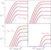 |
Fig. 12 Predicted intensities for the SO2 lines of Table 4. The assumed kinetic temperature and Δv= are 10 K and 1 km s-1, respectively. Units for the density and TB are cm-3 and Kelvin, respectively. Black thin lines correspond to the predictions for the SO2/o-H2 system (this work), red thick lines to the SO2/p-H2 system (this work), and blue dotted lines to SO2-He (rates from Green 1995; extrapolated down to 10 K as indicated in the text). |
3.3. SO2 rotational lines in the millimeter domain
We used the new collisional rates to explore the behavior of the millimeter lines of SO2 that could be detected in cold dark clouds. The calculations were done using the LVG approximation, and the results are shown in Figs. 12 and 13. We selected a kinetic temperature of 10 K, typical of cold dark clouds, and we varied the density between 102 and 108 cm-3 for three different column densities of 1012, 1013, and 1014 cm-2, which could correspond to abundances of 10-8 to 10-10 for a cloud with N(H2) = 1022 cm-2. Among the lines that could be detected in dark clouds in the millimeter domain, we selected those indicated in Table 4.
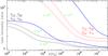 |
Fig. 13 Predicted line intensity ratios for selected lines of interest for the study of dark clouds. The assumed kinetic temperature and Δv= are 10 K and 1 km s-1, respectively. Solid/dashed lines correspond to the case of collisional excitation by ortho/para H2. The results correspond to N(SO2) = 3 × 10¹³ and 3 × 1014 cm-2. The blue thick curve corresponds to N(SO2) = 3 × 1014 cm-2 but using the collisional rates SO2/He of Green (1995). |
Selected SO2 lines in the millimeter domain.
The 313–202 line at 104.029 GHz is the strongest one, and the results show that it thermalized for a density of 105 cm-3 (see Fig. 12). The 515−404 and 524−413 lines are thermalized for a density around 106 cm-3. Like the case for the centimeter wavelength transitions, the predictions are practically the same for ortho and para H2. However, if we use the scaled He-rates, these densities have to be multiplied by a factor 10. The 431−422 line is the weakest of the four lines. Although also thermalized for n(H2) = 106 cm-3, its intensity will only be significant for the highest SO2 column densities.
The line intensity ratios between these transitions are shown in Fig. 13. We can see that the 313−202/515−404 line intensity ratio will be a tracer of the regions of moderate density. However, the 313−202/524−413 one will trace the densest regions of the cloud. No significant differences are found for these ratios as a function of the collider, ortho, or para H2. On the other hand, the line intensity ratios predicted using the He-rates are shifted towards higher densities (one order of magnitude).
To compare our results using our rates with those that could be obtained using those of Green (1995) without extrapolating the rates, we did the same calculations for a temperature of 25 K, the lowest value provided by Green. The results indicate the same behavior as at low temperature; i.e., volume densities a factor ≃ 10 higher are needed for the He-rates to reproduce the predictions obtained using our rates between SO2 and o/p-H2.
4. Summary
We used full quantum scattering calculations to investigate rotational energy transfer in collisions of SO2 with para and ortho H2. The calculations are based on a recent, hightly accurate 5D potential energy surface. Rate coefficients for transitions involving the lowest 31 levels of SO2 were determined for temperatures ranging from 5 to 30 K. It was shown that including H2(j2 = 2) makes a negligible contribution to para-H2 rate coefficients. Rate coefficients with para and ortho-H2 differ by a factor of two on average, and the largest are mainly the rates for collisions with ortho-H2.
The comparison between the present results and the scaled He rates of Green (1995) shows large differences that are found to exceed a factor ten for some transitions, rate coefficients with H2 being always larger than those with He. These discrepancies may be explained by the differences between the potential energy surfaces and by the approximate IOS collisional treatment used by Green for the He-rate calculations.
We used the new rates to predict the behavior of the SO2 lines in the centimeter and millimeter domain. For the lowest frequencies we have found that the line 111−202 should be in absorption against the cosmic background radiation for densities below 104 cm-3. The amount of absorption is directly proportional to the column density of SO2. These predictions have been confirmed with observations using the GBT telescope. We also predict that the line 404−313 will be a maser with a maximum population inversion efficiency for densities around 5 × 103 cm-3. The observation of this line will provide strong constraints on the abundance of SO2 in the medium-density regions of cold dark clouds.
Please note that, to simplify the writing, “rates” refers to “rate coefficients” throughout the paper.
Acknowledgments
The scattering calculations were performed at the IDRIS-CNRS French national computing center (Institut de Développement et des Ressources en Informatique Scientifique du Centre National de la Recherche Scientifique) under project 060883 and on local work stations of the Centre Informatique of Paris Observatory. L.C.-V. was supported in 2006−2008 by
the FP6 Research Training Network “Molecular Universe” under contract number MCRTN-CT-2004-512302 and in 2008−2009 by a grant of the Lavoisier Program of the French Foreign Office Ministry. J. Cernicharo thanks the Spanish MICINN for funding support under grants AYA2006-14786, AYA2009-07304, and the ASTROMOL Consolider project CSD2009-00038. M.-L. Senent also thanks the Spanish MICINN for funding support under grant AYA2005-00702. This research was also supported by the CNRS national program “Physique et Chimie du Milieu Interstellaire”. We would like to thank the GBT staff for support during the observations. The authors wish to acknowledge their friend and colleague Pierre Valiron who actively participated in the work that leads to this paper. Pierre passed away on 31 August 2008, and we dedicate this paper to his memory.
References
- Alexander, M. H., & Manolopoulos, D. E. 1987, J. Chem. Phys., 86, 2044 [NASA ADS] [CrossRef] [Google Scholar]
- Bachiller, R., & Cernicharo, J. 1986, A&A, 166, 283 [NASA ADS] [Google Scholar]
- Brinch, C., Crapsi, A., Hogerheijde, M. R., & Jørgensen, J. K. 2007, A&A, 461, 1037 [NASA ADS] [CrossRef] [EDP Sciences] [Google Scholar]
- Cernicharo, J., & Bachiller, R. 1984, A&AS, 58, 327 [NASA ADS] [Google Scholar]
- Cernicharo, J., & Guélin, M. 1987, A&A, 176, 299 [NASA ADS] [Google Scholar]
- Cernicharo, J., Guélin, M., & Askne, J. 1984, A&A, 138, 371 [NASA ADS] [Google Scholar]
- Cernicharo, J., Bachiller, R., & Duvert, G. 1985, A&A, 149, 273 [NASA ADS] [Google Scholar]
- Daniel, F., Cernicharo, J., Roueff, E., Gerin, M., & Dubernet, M. L. 2007, ApJ, 667, 980 [NASA ADS] [CrossRef] [Google Scholar]
- Dickens, J. E., Irvine, W. M., Snell, R. L., et al. 2000, ApJ, 542, 870 [NASA ADS] [CrossRef] [Google Scholar]
- Dubernet, M.-L., Daniel, F., Grosjean, A., et al. 2006, A&A, 460, 323 [NASA ADS] [CrossRef] [EDP Sciences] [Google Scholar]
- Dubernet, M.-L., Daniel, F., Grosjean, A., & Lin, C. Y. 2009, A&A, 497, 911 [NASA ADS] [CrossRef] [EDP Sciences] [Google Scholar]
- Duvert, G., Cernicharo, J., & Baudry, A. 1986, A&A, 164, 349 [NASA ADS] [Google Scholar]
- Faure, A., Crimier, N., Cecarelli, C., et al. 2007, A&A, 472, 1029 [NASA ADS] [CrossRef] [EDP Sciences] [Google Scholar]
- Fuller, G. A., Ladd, E. F., & Hodapp, K.-W. 1996, ApJ, 463, L97 [NASA ADS] [CrossRef] [Google Scholar]
- Green, S. 1995, ApJS, 100, 213 [NASA ADS] [CrossRef] [Google Scholar]
- Grosjean, A., Dubernet, M.-L., & Ceccarelli, C. 2003, A&A, 408, 1197 [NASA ADS] [CrossRef] [EDP Sciences] [Google Scholar]
- Hogerheijde, M. 2001, ApJ, 553, 618 [NASA ADS] [CrossRef] [Google Scholar]
- Hogerheijde, M., Van Disjoeck, E., Blake, G. A., & van Langevelde, H. J. 1997, ApJ, 489, 293 [NASA ADS] [CrossRef] [Google Scholar]
- Hutson, J. M., & Green, S. 1994, MOLSCAT computer code, version 14, Collaborative Computational Project No. 6 of the Science and Engineering Research Council, United Kingdom [Google Scholar]
- Irvine, W. M., Food, J. C., & Schloerb, F. P. 1983, A&A, 127, L10 [NASA ADS] [Google Scholar]
- Jørgensen, J. K., Schöier, F. L., & van Dishoeck, E. F. 2004, 416, 603 [Google Scholar]
- Lique, F., Cernicharo, J., & Cox, P. 2006, ApJ, 653, 1342 [NASA ADS] [CrossRef] [Google Scholar]
- Lique, F., Senent, M. L., Spielfiedel, A., & Feautrier, N. 2007, J. Chem. Phys., 126, 164312 [NASA ADS] [CrossRef] [PubMed] [Google Scholar]
- Lique, F., Tobola, R., Klos, J., et al. 2008, A&A, 567, 574 [Google Scholar]
- Lique, F., Spielfiedel, A., Feautrier, N., et al. 2010, J. Chem. Phys., 132, 24303 [Google Scholar]
- Lovas, F. J. 1978, J. Chem. Phys. Ref. Data, 7, 1445 [Google Scholar]
- Myers, P. C., Bachiller, R., Caselli, P., et al. 1995, ApJ, 449, L65 [NASA ADS] [CrossRef] [Google Scholar]
- Ohashi, N., Hayashi, M., Ho, P. T. P., & Momose, M. 1997, 475, 211 [Google Scholar]
- Palumbo, M. E., Leto, P., Siringo, C., & Trigilio, C. 2008, ApJ, 685, 1033 [NASA ADS] [CrossRef] [Google Scholar]
- Phillips, T. R., Maluendes, S., & Green, S. 1996, ApJS, 107, 476 [Google Scholar]
- Pickett, H. M., Poynter, R. L., Cohen, E. A., et al. 1998, J. Quant. Spectrosc. & Rad. Transfer, 60, 883, see also JPL Molecular Spectroscopy Catalog: http://spec.jpl.nasa.gov [Google Scholar]
- Schilke, P., Benford, D. J., Hunter, T. R., Lis, D. C., & Phillips, T. G. 2001, ApJS, 132, 281 [NASA ADS] [CrossRef] [Google Scholar]
- Schloerb, F. P., Irvine, W. M., Friberg, P., Hjalmarson, A., & Hoglund, B. 1983, ApJ, 264, 161 [NASA ADS] [CrossRef] [Google Scholar]
- Snyder, L. E., Hollis, J. M., Ulich, B. L., et al. 1975, ApJ, 198, L81 [NASA ADS] [CrossRef] [Google Scholar]
- Spielfiedel, A., Senent, M.-L., Dayou, F., et al. 2009, J. Chem. Phys., 131, 014305 [NASA ADS] [CrossRef] [PubMed] [Google Scholar]
- Takakuwa, S., Mikami, H., Saito, M., & Hirano, N. 2000, ApJ, 542, 367 [NASA ADS] [CrossRef] [Google Scholar]
- Troscompt, N., Faure, A., Wiesenfeld, L., Ceccarelli, C., & Valiron, P. 2009, A&A, 493, 687 [NASA ADS] [CrossRef] [EDP Sciences] [Google Scholar]
- Valiron, P., & McBane, G. C. 2008, MPI and OpenMP extension of MOLSCAT; program repository on: http://www-laog.obs.ujf-grenoble.fr/~valiron/molscat/ [Google Scholar]
- Valiron, P., Wernli, M., Faure, A., et al. 2008, J. Chem. Phys., 129, 134306 [NASA ADS] [CrossRef] [PubMed] [Google Scholar]
- Wernli, M., Wiesenfeld, L., Faure, A., & Valiron, P. 2007a, A&A, 464, 1147; A&A, 475, 391 [NASA ADS] [CrossRef] [EDP Sciences] [Google Scholar]
- Wernli, M., Wiesenfeld, L., Faure, A., & Valiron, P. 2007b, A&A, 475, 391 [NASA ADS] [CrossRef] [EDP Sciences] [Google Scholar]
- Woon, D. E., & Dunning Jr., T. H. 1994, J. Chem. Phys., 100, 2975 [NASA ADS] [CrossRef] [Google Scholar]
- William, H. L., Mas, E. M., Szalewicz, K., & Jeziorski, B. 1995, J. Chem. Phys., 103, 7374 [NASA ADS] [CrossRef] [Google Scholar]
All Tables
SO2 calculated energy levels (in cm-1) compared to values deduced from the JPL molecular spectroscopy catalog in Pickett et al. (1998).
Rate coefficients (in cm3 s-1) for the rotational deexcitation of SO2 by collisions with He (Green 1995, scaled), para-H2 (j2 = 0), para-H2 (j2 = 0,2), ortho-H2 (j2 = 1) at T = 25 Ka.
All Figures
|
Fig. 1 Cross section for excitation by para and ortho-H2 for the 331 → 431 transition as a function of the energy E = Ec + Erot(SO2). Black curve: para-H2(j2 = 0); red curve para-H2 = (j2 = 0,2); blue curve: ortho-H2(j2 = 1). |
| In the text | |
|
Fig. 2 Cross section for excitation by para and ortho-H2 for the 431 → 440 transition as a function of the energy E = Ec + Erot(SO2). Black curve: para-H2(j2 = 0); red curve para-H2 = (j2 = 0,2); blue curve: ortho-H2(j2 = 1). |
| In the text | |
|
Fig. 3 Temperature variation of the de-excitation rate coefficient for transitions with ΔKa = 0. p2 and o1 refer to para and ortho-H2 rate coefficients. |
| In the text | |
|
Fig. 4 Temperature variation of the de-excitation rate coefficient for transitions with ΔJ = 0. p2 and o1 refer to para and ortho-H2 rate coefficients. |
| In the text | |
|
Fig. 5 SO2 rotational levels connected to the initial one (431), denoted by a black diamond. Those marked by a gray disk have a para-H2 collisonal excitation or deexcitation rate above the threshold > 10-12 cm3 s-1, with the area of each gray disk proportional to the rate. Crosses correspond to rates below the threshold. |
| In the text | |
|
Fig. 6 De-excitation rate coefficients of SO2 in collision with para-H2(j2 = 0) as function of rate coefficients with para-H2(j2 = 0,2). The black line indicates equal rates. |
| In the text | |
|
Fig. 7 Rotational levels of SO2 with energies below 13 K. Allowed radiative transitions are indicated by red arrows. The numbers indicate the corresponding Einstein coefficients for spontaneous emission in units of 10-8 s-1. |
| In the text | |
|
Fig. 8 Predicted brightness temperature for the 111 − 202 line of SO2 at 12.256 GHz for different sets of collisional rates. The assumed kinetic temperature and Δv= are 10 K and 1 km s-1, respectively. Black(thin)/red(thick) lines correspond to the excitation of the molecule by o-H2/p-H2 using the collisional rates calculated in this work. Blue(dashed) lines correspond to the predicted intensity when the scaled He-rates of Green (1995) are used. Column densities are indicated and correspond to 3 × 10¹⁴, 1014, 3 × 10¹³, and 1013 cm-2. |
| In the text | |
|
Fig. 9 Predicted brightness temperature for the 404−313 line of SO2 at 29.321 GHz for different sets of collisional rates. The assumed kinetic temperature and Δv= are 10 K and 1 km s-1, respectively. Black(thin)/red(thick) lines correspond to the excitation of the molecule by o-H2/p-H2 using the collisional rates calculated in this work. Blue dotted lines correspond to the predicted intensity when the rates of Green (1995) for the SO2-He system are used. Column densities are indicated and correspond to 3 × 10¹⁴, 1014, 3 × 10¹³, and 1013 cm-2. |
| In the text | |
|
Fig. 10 Raw data for the 111 − 202 line of SO2 obtained towards four dark clouds. Although the data suffer from a high-frequency ripple plus spurious features produced by human-made interferences, the absorption features appear clearly in three of them, TMC1, L1527, and L1489. Processed data are shown in Fig. 11. |
| In the text | |
|
Fig. 11 Observed 111−202 line profile towards TMC1, L1527 and L1489. The raw data without any processing are shown in Fig. 10. The x-axis corresponds to LSR velocity and the y-axis corresponds to the observed antenna temperature. |
| In the text | |
|
Fig. 12 Predicted intensities for the SO2 lines of Table 4. The assumed kinetic temperature and Δv= are 10 K and 1 km s-1, respectively. Units for the density and TB are cm-3 and Kelvin, respectively. Black thin lines correspond to the predictions for the SO2/o-H2 system (this work), red thick lines to the SO2/p-H2 system (this work), and blue dotted lines to SO2-He (rates from Green 1995; extrapolated down to 10 K as indicated in the text). |
| In the text | |
|
Fig. 13 Predicted line intensity ratios for selected lines of interest for the study of dark clouds. The assumed kinetic temperature and Δv= are 10 K and 1 km s-1, respectively. Solid/dashed lines correspond to the case of collisional excitation by ortho/para H2. The results correspond to N(SO2) = 3 × 10¹³ and 3 × 1014 cm-2. The blue thick curve corresponds to N(SO2) = 3 × 1014 cm-2 but using the collisional rates SO2/He of Green (1995). |
| In the text | |
Current usage metrics show cumulative count of Article Views (full-text article views including HTML views, PDF and ePub downloads, according to the available data) and Abstracts Views on Vision4Press platform.
Data correspond to usage on the plateform after 2015. The current usage metrics is available 48-96 hours after online publication and is updated daily on week days.
Initial download of the metrics may take a while.