| Issue |
A&A
Volume 531, July 2011
|
|
|---|---|---|
| Article Number | A1 | |
| Number of page(s) | 9 | |
| Section | Planets and planetary systems | |
| DOI | https://doi.org/10.1051/0004-6361/201016165 | |
| Published online | 30 May 2011 | |
Constraining the structure of the planet-forming region in the disk of the Herbig Be star HD 100546⋆
1
UJF-Grenoble 1/CNRS-INSU, Institut de Planétologie et d’Astrophysique de Grenoble (IPAG) UMR 5274, 38041 Grenoble Cedex 9, France
e-mail: This email address is being protected from spambots. You need JavaScript enabled to view it.
2
Max-Planck-Institut für Astronomie, Königstuhl 17, 69117 Heidelberg, Germany
3
AstroParticule & Cosmologie (APC), UMR 7164, Université Paris Diderot, 10 rue Alice Domon et Léonie Duquet, 75205 Paris Cedex 13, France
4
INAF – Osservatorio Astrofisico di Arcetri, Largo E. Fermi 5, 50125 Firenze, Italy
5
Max-Planck-Institut für Radioastronomie, Auf dem Hugel 69, 53121 Bonn, Germany
6 Laboratoire H. Fizeau, UMR 6525 UMS, CNRS, OCA, Université de Nice Sophia-Antipolis, 06108, Nice Cedex 2, France
Received: 18 November 2010
Accepted: 30 March 2011
Abstract
Context. Studying the physical conditions in circumstellar disks is a crucial step toward understanding planet formation and disk evolution. Of particular interest is the case of HD 100546, a Herbig Be star that presents a gap within the first 13 AU of its protoplanetary disk, a gap that may originate in the dynamical interactions of a forming planet with its hosting disk.
Aims. We seek a more detailed understanding of the structure of the circumstellar environment of HD 100546 and refine our previous disk model that is composed of a tenuous inner disk, a gap and a massive outer disk (see Benisty et al. 2010, A&A, 511, A75). We also investigate whether planetary formation processes can explain the complex density structure observed in the disk.
Methods. We gathered a large amount of new interferometric data using the AMBER/VLTI instrument in the H- and K-bands to spatially resolve the warm inner disk and constrain its structure. Then, combining these measurements with photometric observations, we analyze the circumstellar environment of HD 100546 in the light of a passive disk model based on 3D Monte-Carlo radiative transfer. Finally, we use hydrodynamical simulations of gap formation by planets to predict the radial surface density profile of the disk and test the hypothesis of ongoing planet formation.
Results. The SED (spectral energy distribution) from the UV to the millimeter range, and the NIR (near-infrared) interferometric data are adequately reproduced by our model. We show that the H- and K-band emissions are coming mostly from the inner edge of the internal dust disk, located near 0.24 AU from the star, i.e., at the dust sublimation radius in our model. At such a short distance, the survival of hot (silicate) dust requires the presence of micron-sized grains, heated at ~1750 K. We directly measure an inclination of 33° ± 11° and a position angle of 140° ± 16° for the inner disk. This is similar to the values found for the outer disk (i ≃ 42°, PA ≃ 145°), suggesting that both disks may be coplanar. We finally show that 1 to 8 Jupiter mass planets located at ~8 AU from the star would have enough time to create the gap and the required surface density jump of three orders of magnitude between the inner and outer disk. However, no information on the amount of matter left in the gap is available, which precludes us from setting precise limits on the planet mass, for now.
Key words: stars: individual: HD 100546 / circumstellar matter / techniques: interferometric
Based on observations collected at the VLT (ESO Paranal, Chile) with programs 082.D-0010(A), 083.C-0298(A,B), 083.D-0224(C), 083.C-0146(B), 083.C-0144(A,D), 083.C-0236(A), 075.C-0637(A)
© ESO, 2011
1. Introduction
Studying the physical conditions in circumstellar disks and the processes that rule the evolution of gas and dust provides the context for the formation of planets. It is now clear that several processes are simultaneously acting on the disks at a given time. With the advent of powerful mid- and far-infrared space telescopes such as Spitzer, a new class of objects has been identified, the pre-transitional and transitional disks (e.g., Espaillat et al. 2010). Pre-transitional disks have a typical spectral energy distribution (SED) with a near-infrared excess resulting from the emission of hot dust and gas located in an inner disk, a dip in the mid-infrared range likely caused by a gap, and at longer wavelengths, the signature of an optically thick outer disk.
Log of the observations and associated (u,v) coverage.
HD 100546, well studied already by ISO, is a late Herbig Be star (B9.5Ve) that is now classified as a transitional disk. Located at ~  pc (as measured by Hipparcos, van den Ancker et al. 1998), it has a large-scale disk inclined by ~40° (0° meaning pole-on, this convention will be used throughout the paper) extending up to 4′′ that was first imaged in scattered light (Pantin et al. 2000). Its estimated age of 10 Myr (van den Ancker et al. 1997) corresponds to the timescale on which disks are found to dissipate (Hillenbrand et al. 2008), which suggests that the disk is evolved. Coronagraphic imaging revealed a large-scale envelope (~1000 AU) and a disk extending up to 515 AU with an asymmetric brightness profile (Augereau et al. 2001; Grady et al. 2001). Based on its SED that shows a dominant mid-infrared excess, peaking at 40 μm and with a weak 2–8 μm emission, Bouwman et al. (2003) suggested the presence of an inner hole within 10 AU that could possibly result from the presence of a very low-mass stellar or planetary companion in the disk (20 MJup, Acke & van den Ancker 2006). Nulling interferometry at mid-infrared wavelengths showed that the radial temperature law in the few inner AUs cannot be explained with a continuously flared disk (Liu et al. 2003). Additional evidence of a cavity is provided by means of spectroscopy: HST/STIS observations of H2 emission revealed a hole extending to 13 AU (Grady et al. 2005a), while a lack of 6300 Å [OI] emission inside 6.5 AU is observed (Acke & van den Ancker 2006). Recent CO ro-vibrational observations (Brittain et al. 2009; van der Plas et al. 2009) reported an extended emission with a large inner hole inside ~ 11–13 AU, confirming the status of pre-transitional disk given to HD 100546.
Recent far-infrared and millimetric observations enabled further studies of the gas and dust in the outer disk. Panić et al. (2010) detected pure rotational lines of CO and derived a mass of 10-3 M⊙ of molecular gas in the disk. Their model is consistent with an inclined outer disk (i ~ 40°) in Keplerian rotation that extends out to 400–500 AU in radius. The Herschel Space Observatory detected several additonal molecular lines as well as forbidden atomic lines ([CII] and [OI]) that probably result from photo-dissociation by stellar photons (Sturm et al. 2010).
On the other hand, very little is known about the inner disk. Far ultraviolet (FUV) observations of molecular hydrogen (Lecavelier des Etangs et al. 2003; Martin-Zaïdi et al. 2008) imply that the observed gas lies very close to the central star. Although these observations give evidence that the inner 1.5 AUs are not cleared of gas, clues are still missing for a firm conclusion about the location of this gas (FUV-driven photoevaporative wind from the surface layers of the disk, gas in an inner disk...). However, the near-infrared (NIR) excess, the emission from gas located as close to the central star as 0.5 AU (Acke & van den Ancker 2006), as well as the signs of accretion (Deleuil et al. 2004) all suggest that the innermost AUs are not empty.
This was confirmed by interferometric measurements in the K-band that spatially resolved the dust emission at the sub-AU scale (Benisty et al. 2010, hereafter B10). The authors, based on two visibility measurements at 2.2 and 8.7 μm, proposed a disk model that includes an inner disk, a gap, and an optically thick outer disk that are able to reproduce the SED and the visibilities. See their Fig. 3 for a sketch of the disk configuration. Benisty et al. (2010) considered a stellar luminosity of 22 L⊙ to reproduce the photometric measurements at the shortest wavelengths, assuming a null Av and a normal Rv = 3.1 extinction law, while other authors previously used a higher value of 32 L⊙ using a non-zero Av but an anomalous extinction law, Rv ~ 5.1 (van den Ancker et al. 1997).
Owing to the small number of interferometric measurements used in B10, some questions remained unsolved. What is the exact structure of the inner disk? Is it asymmetric and puffed up, or rather smooth? Is there any hot matter located inside the dusty rim that could emit at shorter wavelengths? Are the inner and outer disks coplanar? Could the presence of a sub-stellar companion be constrained?
In this paper, we present new spectro-interferometric measurements obtained in the K-band, as well as the first spatially resolved measurements in the H-band and first closure phase measurements for HD 100546. We build a complete SED from previously published photometric and spectroscopic data, and reassess the stellar luminosity in our model. Based on the extensive dataset, we revisit the disk morphology and study the effects of a putative planetary companion on the disk structure and evolution. In Sect. 2 we present the observations and the data processing. In Sect. 3 we model the SED and interferomeric data. In Sect. 4 we use hydrodynamical simulations to predict the surface density profile in the disk when a planet carves a gap into it. Section 5 is the summary.
2. Observations and data processing
2.1. Interferometry
HD 100546 was observed at the Very Large Telescope Interferometer (VLTI; Schöller 2007), using the AMBER instrument that allows the simultaneous combination of three beams in the near-infrared (Petrov et al. 2007). It delivers spectrally dispersed interferometric observables: visibilities, closure phases, and differential phases. In the following, we present H- and K-band observations taken in the low spectral resolution mode (LR; R ~ 30) with the 1.8 m Auxiliary Telescopes (ATs). The data were obtained during several guaranteed time observation programmes. HD 100546 was observed with 11 different baselines of four VLTI configurations during eight nights from January to May 2009. The longest (projected) baselines achieved for the H- and K-band observations are ~92 and ~127 m, respectively, corresponding to a maximum angular resolution of λ/B ~ 3.9 mas and 3.6 mas, respectively. We use the VLTI nomenclature to identify the different configurations. A summary of the observations used in this paper is given in Table 1. In addition to HD 100546, calibrators (HD104479, HD100901, HD77049) were observed to correct for instrumental effects. Their properties can be found in Table 2. All observations were performed without the fringe-tracker FINITO.
The data reduction was performed following standard procedures described in Tatulli et al. (2007) and Chelli et al. (2009), using the amdlib package, release 3.0b4, and the yorick interface provided by the Jean-Marie Mariotti Center1. Raw spectral visibilities and closure phases were extracted for all the frames of each observing file. A selection of 80% of the highest quality frames was made to overcome the effects of instrumental jitter and unsatisfactory light injection. Calibration of the AMBER+VLTI instrumental transfer function was done using measurements of the calibrators, after correcting for their diameter. Finally, calibrated visibilities and closure phases were averaged over the wavelength range of each band (H: from 1.5 to 1.8 μm; K: from 2.0 to 2.4 μm), to obtain broad-band observables. Because of the combined effects of an intrinsically lower flux of the source and of a lower instrumental sensitivity, the performance of AMBER is worse in the H-band than in the K-band. As a consequence, our H-band data are of lower signal-to-noise ratio, which translates into two effects: (i) the visibility points show a larger scatter in the H-band, and (ii) we were unable to estimate the H-band closure phase for the longest baselines where the source is almost fully resolved. The lower signal-to-noise ratio of the H-band data also explains the lower number of data points in the lower panel of Fig. 1, especially at long baseline lengths where the visibilities are lower.
Stellar and calibrator properties.
2.2. Spectroscopy
FUSE spectrum: although HD 100546 was observed twice with Fuse, in 2000 and in 2002 (Martin-Zaïdi et al. 2008), we only considered the exposures of 2002 that have the best signal-to-noise ratio. The observations were all made in the time-tagged mode, using the 30′′ × 30′′ LWRS aperture at a resolution of about 15 000. The total exposure time was split into several sub-exposures that were co-aligned using a linear cross-correlation procedure and added segment by segment. The individual spectra (905–1187 Å) were processed with the CALFUSE pipeline processing software v3.0.7 (Sahnow et al. 2000; Dixon et al. 2007), to correct for instrumental effects.
UVES spectrum: the star was observed on 2005 March 21, with UVES (Dekker et al. 2000), a cross-dispersed echelle spectrograph mounted at the VLT. For these observations, the blue arm was used with a spectral coverage between ~3700 Å and 5000 ÅẆe used no image slicer, low gain with a 1 × 1 binning of the CCDs and a slit width of 0.4′′ providing the maximum resolution of ~80 000. Wavelength calibration frames were taken with a long slit and a ThAr arc lamp. The spectrum was reduced using the UVES pipeline v3.2.0 (Ballester et al. 2000) available on the ESO Common Pipeline Library. The spectrum was corrected for the Earth’s rotation to shift it in the heliocentric rest frame. No standard star is available to provide an accurate flux calibration. We scaled the UVES flux to the IUE one, which agrees well with the best photospheric model for HD 100546 (see Sect. 3.1).
IUE spectra: we used archived IUE spectra at short (SWP: 1150–1975 Å) and long (LWP: 1850–3350 Å) wavelengths to cover the entire UV band. The spectra, of high signal-to-noise ratio, were obtained with the large aperture (10′′ × 20′′) and the high-dispersion mode which produces a two-dimensional echelle spectrum containing approximately 60 orders, with a resolution of roughly 0.2 Å.
2.3. The spectral energy distribution
The photometric data used in the SED are the same as in B10. They were retrieved from the literature. They include photometry from ground-based telescopes in the optical and NIR, 2MASS data, mid-infrared photometry from the IRAS and ISO satellites (Ardila et al. 2007; Henning et al. 1994; Grady et al. 2001; Malfait et al. 1998; Sturm et al. 2010). These are shown as black dots in Fig. 2. We also included spectra from the FUSE, IUE, and ISO archives.
3. Modeling
3.1. Stellar properties
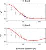 |
Fig. 1 Broad-band squared visibilities with (1σ) error bars shown against effective baseline for the K-band (upper panel) and the H-band (lower panel). The H-band plot shows less data points because of a lower number of V2 measurements above the required S/N ratio threshold. The predictions of the best uniform ring model are overplotted in solid line. The filled blue points correspond to the visibilities used in the B10 paper. |
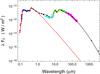 |
Fig. 2 Observed spectral energy distribution of HD 100546 compared to our best-model prediction (full black line, Teff = 10 500 K, 26 L⊙, Av = 0.2, Rv = 5.5). The photosphere is shown as a red line. The photometric data used in B10 are represented by black dots. The binned FUSE spectrum is plotted with red dots, the binned IUE spectrum with blue dots, the archival ISO data are plotted with cyan dots for ISO-PHOT, green dots for ISO-SWS, and magenta dots for ISO-LWS. The IRAS-LRS data are represented by yellow dots. |
Various estimates of the fundamental parameters of HD 100546 have been proposed over the past 15 years. The effective temperature found in the literature varies from 10 000 to 11 000 K, estimates of the visual extinction toward this star range from Av = 0.0 to Av = 1.03, and the stellar luminosity estimates range from 22 to 32 L⊙ (e.g., Thé et al. 1994; van den Ancker et al. 1998; Valenti et al. 2000; Acke & van den Ancker 2006). These significant differences have motivated a thorough modeling of the photosphere. We started considering photospheric models from the Kurucz grid of LTE models (Kurucz 1979; Castelli & Kurucz 2004). The sub-grid thus obtained samples the parameter space 9000 K ≤ Teff ≤ 12 000 K with 250 K steps and 3.5 ≤ log g ≤ 5.0 with 0.25 dex steps. Then, synthetic spectra were calculated in NLTE using the Synspec package of Hubeny & Lanz (1995). This code allows for an approximate NLTE treatment of lines with LTE photospheric models2. The result of this stage is to determine the LTE model that provides the best fit to the observed spectra. The model assumes a solar composition, a helium abundance, Y = He/H = 0.1 by number, and a microturbulent velocity, ξt = 2 km s-1. For details of the modeling method of FUV and UV spectra of Herbig stars, we refer the reader to Bouret et al. (2003). The best-fit model provides the following stellar properties: Teff = 10 500 K, log g = 4.0 and v sin i = 55 km s-1.
The stellar luminosity was calculated from Teff and using HIPPARCOS parallaxes (van den Ancker et al. 1998; Bertout et al. 1999) and bolometric corrections using the method described in Bessell et al. (1998): 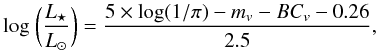 (1)where π is the parallax in arcseconds, mv is the V-band magnitude of the object, and BCv, the bolometric correction. We found a luminosity of 25.9
 L⊙. All previously published values are within 2σ of our estimate. In the following, we use 26 L⊙. We note that B10 used a stellar luminosity of 22 L⊙ and a null extinction, assuming a normal (Rv = 3.1) extinction law. In addition, they had a limited sampling of the stellar flux at wavelengths shorter than 3000 Å. A comparison with the stellar models of Siess et al. (2000) suggests that this luminosity is probably too low, unless the metallicity of HD 100546 is Z = 0.01 (half solar).
The dataset used by B10 can also be fitted properly with a higher luminosity, e.g., 32 L⊙ as in van den Ancker et al. (1997) or with 26 L⊙ (this work) but with a non-zero and anomalous extinction (Av ~ 0.2−0.3 and Rv ~ 5.5). The anomalous extinction law is needed to fit the flat UV spectrum now included in the SED. We note that the photospheric model and extinction curve we use lead to a slight underestimation of the UV flux near 100nm. We suggest this excess is a consequence of the accretion process still going-on for HD 100546. This has no significant impact on the continuum energy budget and continuum emission from the dust disk because the flux densities involved are too low by a large factor.
3.2. Location of the near-infrared emission
To derive the basic characteristics of the NIR emission, we first consider a simple geometrical model made of a ring of uniform surface brightness to roughly estimate the location of the emission. We choose a ring instead of, e.g., a uniform disk because the bulk of the emission is expected to come from the inner rim of the dusty disk, as shown in B10. The ring model has three degrees of freedom, namely the ring inner radius Rd, inclination id and position angle PAd. The ring thickness is fixed at 20% of the radius. The modeled visibility can be written as ![Mathematical equation: \begin{equation} V^{[H,K]}_{\rm ring} = \frac{V_{\ast}F^{[H,K]}_{\ast} + V_{\rm ex}F^{[H,K]}_{\rm ex}}{F^{[H,K]}_{\ast} + F^{[H,K]}_{\rm ex}}, \end{equation}](/articles/aa/full_html/2011/07/aa16165-10/aa16165-10-eq52.png) (2)with V ∗ = 1 (unresolved central star) and
(2)with V ∗ = 1 (unresolved central star) and ![Mathematical equation: \hbox{$F^{[H,K]}_{\rm ex}/(F^{[H,K]}_{\ast}+F^{[H,K]}_{\rm ex})$}](/articles/aa/full_html/2011/07/aa16165-10/aa16165-10-eq54.png) the NIR excess, i.e., the excess over the stellar flux divided by the total flux in the H- and K-band respectively. Modelling the stellar photosphere emission as described in Sect. 3.1, we estimate H- and K-band excesses of ≃ 0.53 and ≃ 0.75.
the NIR excess, i.e., the excess over the stellar flux divided by the total flux in the H- and K-band respectively. Modelling the stellar photosphere emission as described in Sect. 3.1, we estimate H- and K-band excesses of ≃ 0.53 and ≃ 0.75.
An independent fit of the H- and K-band visibilities for HD 100546 shows that the continuum emission in both bands comes from the same location, within the uncertainties. We therefore performed a classical χ2 minimization using the complete H- and K-band visibility datasets together. We constrain the NIR-emitting region to be located at Rd = 0.25 AU ± 0.02 AU, which reinforces the estimation made in our previous study (Rd = 0.26 AU; B10). We note that this estimation is independent of the continuum emission mechanism, it is in particular independent of the dust properties in the disk.
Because the observations provide a good coverage of the spatial frequencies (see Table 1) we are also able to estimate the inclination and position angle of the inner disk. They are id = 33° ± 11° and PAd = 140° ± 16° respectively. The best ring model is shown in Fig. 1, together with the squared visibilities plotted against the effective baseline length. The effective baseline length is defined as 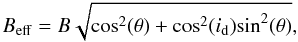 (3)where θ is the angle between the baseline direction and the major axis of the disk, and id is the disk inclination (Tannirkulam et al. 2008). This representation is useful to show a large dataset in a concise way once the inclination and position angles of the disk are known. Our estimates, relevant for the inner disk, agree well with the previously published values of both the inclination and position angles of the disk measured at larger scales (e.g., Ardila et al. 2007). This result suggests that the inner and outer disks of HD 100546 are most likely coplanar – as implicitly assumed in B10 – or very close to it. This is unlike the case of HD 135344 B for example, another transitional disk (Grady et al. 2009). In the rest of this paper we will use a single inclination and position angle for the whole disk, adopting the values commonly used in previous modeling, namely 42° and 145°, respectively.
We remark that if our fit is good for the long (≳ 30 m) effective baselines (i.e., for angular resolution better than ~ 12 mas), our simple ring model is systematically too high with respect to the visibilities at short baselines. Although most of the NIR emission is located around 0.25 AU, this may indicate that there is some extra extended emission not included in the ring model. The origin of this extended emission will be discussed in the next section, together with our radiative transfer disk model that describes the disk environment of HD 100546.
3.3. Disk structure
Best-model parameters.
Radiative transfer with MCFOST: going beyond the simple geometrical ring model, we used the Monte Carlo-based 3D radiative transfer code MCFOST (Pinte et al. 2006, 2009) to compute the SED and NIR images of HD 100546. Visibilities and closure phases are computed from the NIR model images. Here, we refine the model developed in B10 that was based on one visibility measurement. In particular, we use a higher stellar luminosity of 26 L⊙ (see, Sect. 3.1).
The disk is similarly composed of (i) an inner dusty disk with an inner edge at 0.24 AU; (ii) a gap between 4 AU and 13 AU, necessary to reproduce the dip in the SED; (iii) a surface layer (over the outer disk) of small grains; and (iv) an outer disk from 13 AU to 500 AU holding most of the mass (see the sketch of the disk in Fig. 3 of B10). It is difficult to provide reliable error bars for all these values without a full exploration of the parameter space. But the uncertainties, or validity ranges, in particular regarding the position and size of the gap, were discussed in B10 (see Sect. 5). Their discussion is still valid.
Considering our larger dataset and the change in the stellar luminosity, some of the B10 model parameters need to be slightly adjusted. The location of the inner rim is slightly decreased from 0.26 to 0.24 AU to better match the visibilities. We also reduced the mass of both the inner disk and of the surface layer (see Table 3) to reproduce the NIR excess as well as the MIR bump in the SED. The outer disk now extends up to 500 AU, instead of 350 AU, following recent CO line observations by Panić et al. (2010). We modified the outer disk mass accordingly. In order to generate the large silicate emission feature seen in the SED at 10 μm, we used amorphous olivine grains (Dorschner et al. 1995) for the composition of the surface layer, whereas the rest of the disk is made of astronomical silicate grains (Draine & Lee 1984), as in B10. The remaining parameters such as density profile, scale height, flaring and grain sizes were kept unchanged. The parameters are summarized in Table 3. This model provides an adequate fit of the SED from the UV to the millimeter range, as shown in Fig. 2.
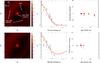 |
Fig. 3 K-band (top) and H-band (bottom) MCFOST modeling of HD 100546. From left to right: NIR images (normalized intensity to one at maximum, in logarithmic scale), visibility (red solid lines) and closure phase (red crosses), compared with the interferometric observations (black circles and error bars). In the middle panels, the “kink” in the model visibility curves at B ~ 10 m is a real feature caused by the sharp inner edge of the outer disk. |
Figure 3 compares the model predictions with the observations. The models agree well with the entire set of H- and K-band visibilities and closure phases. The “kink” in the model visibility curves at B ~ 10 m is caused by the outer disk that has a sharp inner edge and with a finite sampling of the baselines in the models. Increasing the sampling makes the curve smoother, but the “kink” remains. A further demonstration of this can be seen in Fig. 4 (top row, middle panel), where the “kink” disappears when only the inner disk is considered in the field-of-view of the interferometer.
In addition to the visibilities that probe the inner rim location and the properties of the dust it contains, we now discuss the first closure phase measurements of HD 100546. The closure phase is related to the level of asymmetry of the source, here of the NIR continuum emission. Roughly, the values of the closure phases, given in radians, give the ratio between the asymmetric and symmetric fluxes for the corresponding telescope triplet (Monnier 2000). As theoretically expected (Lachaume 2003), the departure from centro-symmetry becomes significant for the closure phase for the longest baselines only, i.e., when the source is well resolved. In our case, with Bmax = 127 m we find a closure phase signal of ~5−10° in the K-band, whereas it is compatible with 0° in the H-band. Recall, however, that the uncertainties are larger and there is a lack of visibilities at very long baselines at H.
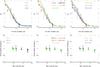 |
Fig. 4 K-band MCFOST modeling of visibility (top) and closure phase in degrees (bottom) for various values of model parameters. Left: various stellar luminosities are compared: 22 L⊙ (green), 26 L⊙ (red), and 32 L⊙ (blue). Middle: effect of the field-of-view when using the AT (red) or UT (black) telescopes. With the latter, only the inner disk of HD 100546 is seen, which is shown in green. The black and green curves lie on top of each other, as expected. Right: the interferometric observables are plotted for different locations of the inner edge of the outer disk, Rin,2 = 9 AU (blue), 13 AU (red), and 17 AU (green). |
Properties of the inner disk: from the data we constrain the location of the disk inner edge at r ~ 0.24 AU from the star. Assuming silicate grains, the inner disk is composed of micron-size particles whose albedos make the scattered light an important part (~30%) of the disk total K-band emission, as discussed in B10. Fairly large grains need to be used (i.e., with amax = 5 μm) to make them survive (i.e., not sublimate too fast) at the inner edge of 0.24 AU, a value imposed by the interferometric observations. Because of the higher stellar luminosity than the one used in B10, we find a temperature for the hottest grains of ~1750 K. We note that this value is on the warm side for silicate grains but we did not attempt to use different compositions. We did not explore either the possiblity that much larger grains be present in the inner disk because their contribution to the disk emission in the NIR is not dominant with respect to the grains used here. Because of the small NIR excess in the SED, we find that the inner disk must be tenuous, with a dust mass of ≃1.75 × 10⁻¹⁰ M⊙.
We find an integrated radial optical depth of τ ≃ 10 (in the I-band) in the equatorial plane of the inner disk. Because it is opaque, depending on its geometrical thickness it may (or may not) cast a shadow and may (or not) significantly modify the temperature structure of the outer disk, hence its scale height. We verified that the scale height profiles used in our parametric models agree with a disk in hydrostatic equilibrium. To check this, we calculated the hydrostatic scale height of a vertically isothermal disk, consistent with the vertical Gaussian density profiles we used, and used the two extreme temperatures found at each radii to bound the scale height of the actual disk. As a minimum temperature for each radius we used the temperature of the disk midplane, the maximum temperature being estimated at the disk surface. We find that the scale height of the outer disk (i.e., H = 12 AU at r = 100 AU) falls between the two estimates, which suggests that the inner disk does not dramatically modify the structure of the outer disk. We note that the scale height of the inner disk (6 AU at 100 AU) is slightly too large, by about 30%.
The measured closure phase value of ~5–10° in the K-band is well reproduced by our model. It is a direct consequence of the anisotropic scattering of starlight by the dust in the inner disk. The phase function of the dust grains in our model has an asymmetry factor g ~ 0.6 (g = 0 is isotropic scattering and g = 1 is fully forward-scattering). The forward-throwing nature of the light scattering process in our model directly results in the asymmetry of the NIR brightness distribution because the disk is inclined. Note also that the closure phase signal is entirely caused by the inner disk, because the outer disk is too faint to contribute at K-band, as shown in Fig. 4 (middle). The outer disk has a different impact on the visibilities, see below. We remark here that we do not need to invoke the presence of a “puffed-up” inner rim (e.g., Dullemond et al. 2001; Isella & Natta 2005) to reproduce the interferometric data because the scale height of the inner rim follows the smooth law defined for the whole inner disk, i.e., H(r) = H0(r/r0)β. In our model we thus have H(Rin) = 0.015 AU corresponding to a ratio H/R of 0.06 for the inner rim, this is a factor 2 to 4 smaller than the values of H/R ~ 0.1−0.25 that are typically expected when the rim is puffed-up and vertical (Dullemond et al. 2001). Monnier et al. (2006) showed that sharp “puffed-up” inner rims are expected to produce large closure phase signals as soon as they are resolved enough. In our case, the value of the inner rim diameter (0.48 AU) in units of fringe spacing λ/Bmax is ~1.3, a value for which substantial closure phases of ≳ 40° would be expected (see Monnier et al. 2006, Fig. 22). Such high values are clearly ruled out by our data. A sharp “puffed-up” inner rim for HD 100456 is unlikely.
The closure phase signal is also very sensitive to the value of the flux ratio between the star and the disk. Because the ratio will vary with the stellar luminosity, a careful determination of this parameter is essential. The study of the closure phase is a good way to cross-check our luminosity estimation of Sect. 3.1. Figure 4 (left) shows the behavior of the (visibility and) closure phase for L ⋆ = 22 L⊙, 26 L⊙, and 32 L⊙, including the values used in the literature. While the visibility profile does not change significantly with the luminosity, the closure phase increases from a few degrees to 15° as the stellar luminosity decreases. Such analysis indirectly confirms that the luminosity of HD 100546 must indeed lie in the [22,32] L⊙ range. More accurate data would be of great interest to reduce this range of validity.
Gap and outer disk: the Auxiliary Telescope’s field of view of λ/D ≃ 250 mas ≡ 25 AU enables us to probe the outer environment of HD 100546, that is, the gap and the outer disk. This extended emission within the field of view directly impacts on the visibility profile at short baselines, as shown in Fig. 4 (middle and right). Including the emission from the outer disk in the model and the field of view better reproduces the visibilities at short-baselines – despite their scatter – than the ring model alone. Typically, with short baselines of a few tens of meters, the interferometer becomes mostly sensitive to the location of the inner edge of the outer disk, as emphasized by Fig. 4 (right). This suggests that the gap must end somewhere between 9 AU and 17 AU. Unfortunately, the scatter in the data does not allow for a better estimation of this parameter.
Interestingly enough, the outer part of the disk would not have been traced with the 8 m Unit Telescopes of the VLTI because it lies outside its field-of-view (λ/D ≃ 60 mas ≡ 6 AU). This points out the importance of the auxiliary telescopes, not only in terms of adding baseline capabilities to that of the UTs, but also in terms of field-of-view for tracing potential extended emission. Indeed, lower visibilities at short baselines with respect to the uniform ring case were also measured for other Herbig AeBe stars (Monnier et al. 2006) and were interpreted as resulting from an extended halo. Our model shows that the scattered light emission from the outer part of a flared disk (even when continuous), a contribution that is usually neglected when modeling the K-band emission, can naturally and easily explain this fairly common feature.
4. Hydrodynamical simulations of gap formation and inner disk evolution
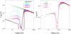 |
Fig. 5 Left: evolution of the density as function of radius in the case of a 6 Jupiter-mass planet. The solid line indicates the density profile used in our model. Right: final density profile as a function of the disk radius for various planet masses. |
It is well documented that a planet in a disk is expected to carve a gap, a trench, in its density profile. Numerous studies exist to study the formation of these gaps by planets via numerical simulations (Bryden et al. 1999; Kley 1999; Nelson et al. 2000; Varnière et al. 2004), but none to our knowledge has focused on trying to reproduce the density jump values needed to match the observations. In this paper, our goal is not to revisit the gap formation mechanism but rather to verify whether a planet embedded in the disk of HD 100546 can explain the large jump in the surface density profile observed on both sides of the gap. To do so, we carried out a series of 2D simulations involving planets of various masses and opening disk gaps. We have made several assumptions and simplifications: circular orbit for the planet, constant accretion rate onto the star over the its full lifetime and equal to the present day accretion rate, the accretion rate in the disk is the same as onto the star and the same at all radii in the disk. However, we have run the numerical simulations sufficiently long to let the inner disk evolve until steady-state is reached. Following Acke & van den Ancker (2006), the lowest planet mass estimate based on the local disk thickness is about 1 Jupiter mass, we therefore started our study with a one Jupiter-mass planet.
To reproduce the density jumps, several mechanisms are competing in the inner region. These are (i) The accretion onto the star; for HD 100546 we have an estimated accretion rate of ~10-9 M⊙/yr (Deleuil et al. 2004; Grady et al. 2005b). This will tend to deplete the inner region, which in turn needs to be replenished. Indeed, with the estimated mass available in the inner region and the observed accretion rate, the inner region should empty itself in less than one year. (ii) The planet “pushes” the gas in the inner region during the creation of its gap. This is a transitory event and occurs soon after the planet formation, it is not part of the steady state we are looking for. (iii) Some material from the outer disk can flow accross the gap, cross the planet’s orbit, and replenish the inner region.
To reproduce the density jump suggested by the observations of HD 100546, one needs to reproduce a surface density for the inner disk that is about three orders of magnitude lower than the surface density just outside of the gap. Ideally, it also needs to produce the proper gap width, i.e., between about 4 and 13 AU.
4.1. Hydrodynamic code and simulation setup
To cover a sufficiently long time-span in the simulation we used the algorithm FARGO (Masset 2000, 2002), which eliminates the azimuthal velocity from the computation of the Courant-Friedrich-Lévy condition. This speeds up the computation and facilitates the study of the long-term disk evolution. Then, to follow the disk over several orders of magnitude in radius to see how the density evolves close to the star as well as outside, we used the code FARGO-2D1D (Crida et al. 2007), which is an extension of the standard version of FARGO, where the 2D grid is surrounded by a simplified 1D grid made of elementary rings that are non azimuthally resolved. It aims at studying and taking into account the general evolution of the disk in the simulations of planet-disk interactions.
We ran several simulations to find and optimize the planet mass needed to create the required density jump. A planet will open a gap near its Lindblad resonance located at 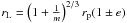 where m is the mode of the Lindblad resonance, rp the position of the planet and e the eccentricity of the orbit. To obtain the outer edge at ~ 13 AU, we placed the planet at 8 AU. We set up the 2D disk around it to capture the 2D structure of the wave. The 2D disk runs from 4 to 20 AU and the 1D disk extends from 0.1 AU to 150 AU3 to reproduce the global behavior of the whole region.
4.2. Simulated density profile: evolution with time
In Fig. 5 (left) we follow the time evolution of the surface density in the first 100 AU of the disk for a 6 Jupiter-mass planet. Such a planet produces a surface density jump of the correct amplitude: the inner disk surface density drops by three orders of magnitude in about 200 000 years, confirming that a 6 MJup planet located at 8 AU can carve the disk of HD 100546 with the proper surface density jump across the gap.
Figure 5 (right) shows that most planet masses are able to reproduce the strong density jumps imposed by the observations. The only differences are the time required to reach that state, the amount of mass left in the gap, and the width of the gap. The main parameters that regulate how much mass is left in the inner region are the accretion rate onto the star and the disk viscosity. If we can estimate the accretion rate from observation, it is a lot harder to have access to the local disk viscosity. We thus adopted an ad hoc value of the viscosity that was successfully used for previous simulations (see for example Quillen et al. 2005) and aim only at reproducing the density jump. This does not allow us to provide a lower limit for the mass of the putative planet because the longest timescale is well within the age of the system and so far we do not have constraints on the mass inside the gap.
Further remarks can be made regarding these numerical results. It is interesting to note that the density profile of the inner region becomes flat early on (before 10 000 years) owing to the accretion onto the star. It becomes flatter than the r-1 power-law used in our model. However, as mentioned above, the slope of the density profile is not well constrained by the current observations. We verified that radiative transfer models that use an inner disk with a flat inner density profiles (i.e., constant with radius) also match the interferometric data and SED.
Also, during the 700 000 years of the simulation time span the planet has a slow migration from 8 to about 7 AU. This slightly moves the outer edge of the gap but it remains within the observational limit. However, in all simulations the gap width appears too narrow compared to the surface density profile estimated from the data. We did not try to solve this question. We can only suggest that an elliptical orbit for the planet may help to broaden the gap. Also, HD 100546 is significantly older than the final time of each simulations. It is therefore difficult to estimate how much wider the gap would have grown in the simulations by the age of the star. Finally, we also note that the full extent of the inner disk, in particular its outer radius, are not well contrained by the data. Rout of the inner disk, which defines the inner boundary of the gap, could be moved outward somewhat depending on the exact vertical density profile. We refer the reader to a forthcoming paper for a more detailed comparison of the profiles from the hydrodynamical simulations and those from data fitting. For now, we only note that a planet can produce the observed surface density jump across the gap.
5. Summary
The main results of our paper are summarized below:
-
using the AMBER/VLTI interferometer in H- and K-band, we spatially resolved the near-infrared emission region of HD 100546. Most of this emission arises from the inner edge of its inner disk located at 0.24 ± 0.02 AU from the star;
-
a puffed-up rim in the inner disk appears unlikely because of the small closure phase signal;
-
for the first time, our observations also constrain the inclination and the position angle of its inner disk. We find i = 33° ± 11° and PA = 140° ± 16°, which suggests that the inner and outer disks are likely coplanar;
-
we described the circumstellar environment of HD 100546 in the light of a passive disk model based on 3D Monte-Carlo radiative transfer. Our model is composed of (i) a tenuous inner disk with a dust mass of ~1.75 × 10⁻¹⁰ M⊙ from 0.24 AU to ~4 AU; (ii) a gap devoid of dust; and (iii) a massive outer disk with a dust mass of ~4.3 × 10⁻⁴ M⊙ extending from ~13 AU to ~500 AU. The model reproduces both the SED and the interferometric observations adequately;
-
we show from hydrodynamical simulations that disk-planet interactions with a planet located at ~8 AU are able to reproduce the observed density jump between the inner and outer disks, across the gap.
We ran test simulations with different sizes of both disks to validate the range of the 2D vs. 1D part of the domain and found no major differences.
Acknowledgments
We thank the VLTI team at Paranal. C. Pinte acknowledges funding from the European Commission seventh Framework Program (contracts PIEF-GA-2008-220891 and PERG06-GA-2009-256513). F. Ménard, C. Pinte, C. Martin-Zaïdi and W.-F. Thi acknowledge PNPS, CNES and ANR (contract ANR-07-BLAN-0221) for financial support.
References
- Acke, B., & van den Ancker, M. E. 2006, A&A, 449, 267 [NASA ADS] [CrossRef] [EDP Sciences] [Google Scholar]
- Ardila, D. R., Golimowski, D. A., Krist, J. E., et al. 2007, ApJ, 665, 512 [NASA ADS] [CrossRef] [Google Scholar]
- Augereau, J. C., Lagrange, A., Mouillet, D., & Ménard, F. 2001, A&A, 365, 78 [NASA ADS] [CrossRef] [EDP Sciences] [Google Scholar]
- Ballester, P., Modigliani, A., Boitquin, O., et al. 2000, The Messenger, 101, 31 [NASA ADS] [Google Scholar]
- Benisty, M., Tatulli, E., Ménard, F., & Swain, M. R. 2010, A&A, 511, A75 [NASA ADS] [CrossRef] [EDP Sciences] [Google Scholar]
- Bertout, C., Robichon, N., & Arenou, F. 1999, A&A, 352, 574 [NASA ADS] [Google Scholar]
- Bessell, M. S., Castelli, F., & Plez, B. 1998, A&A, 333, 231 [NASA ADS] [Google Scholar]
- Bouret, J., Martin, C., Deleuil, M., Simon, T., & Catala, C. 2003, A&A, 410, 175 [NASA ADS] [CrossRef] [EDP Sciences] [Google Scholar]
- Bouwman, J., de Koter, A., Dominik, C., & Waters, L. 2003, A&A, 401, 577 [NASA ADS] [CrossRef] [EDP Sciences] [Google Scholar]
- Brittain, S. D., Najita, J. R., & Carr, J. S. 2009, ApJ, 702, 85 [NASA ADS] [CrossRef] [Google Scholar]
- Bryden, G., Chen, X., Lin, D. N. C., Nelson, R. P., & Papaloizou, J. C. B. 1999, ApJ, 514, 344 [NASA ADS] [CrossRef] [Google Scholar]
- Castelli, F., & Kurucz, R. L. 2004, [arXiv/astro-ph:0405087] [Google Scholar]
- Chelli, A., Utrera, O. H., & Duvert, G. 2009, A&A, 502, 705 [NASA ADS] [CrossRef] [EDP Sciences] [Google Scholar]
- Crida, A., Morbidelli, A., & Masset, F. 2007, A&A, 461, 1173 [NASA ADS] [CrossRef] [EDP Sciences] [Google Scholar]
- Dekker, H., D’Odorico, S., Kaufer, A., Delabre, B., & Kotzlowski, H. 2000, in SPIE Conf. Ser. 4008, ed. M. Iye, & A. F. Moorwood, 534 [Google Scholar]
- Deleuil, M., Lecavelier des Etangs, A., Bouret, J., et al. 2004, A&A, 418, 577 [NASA ADS] [CrossRef] [EDP Sciences] [Google Scholar]
- Dixon, W. V., Sahnow, D. J., Barrett, P. E., et al. 2007, PASP, 119, 527 [NASA ADS] [CrossRef] [Google Scholar]
- Dorschner, J., Begemann, B., Henning, T., Jaeger, C., & Mutschke, H. 1995, A&A, 300, 503 [NASA ADS] [Google Scholar]
- Draine, B. T., & Lee, H. M. 1984, ApJ, 285, 89 [Google Scholar]
- Dullemond, C. P., Dominik, C., & Natta, A. 2001, ApJ, 560, 957 [NASA ADS] [CrossRef] [Google Scholar]
- Espaillat, C., D’Alessio, P., Hernández, J., et al. 2010, ApJ, 717, 441 [NASA ADS] [CrossRef] [Google Scholar]
- Grady, C. A., Polomski, E. F., Henning, T., et al. 2001, AJ, 122, 3396 [NASA ADS] [CrossRef] [Google Scholar]
- Grady, C. A., Woodgate, B., Heap, S. R., et al. 2005a, ApJ, 620, 470 [Google Scholar]
- Grady, C. A., Woodgate, B., Heap, S. R., et al. 2005b, ApJ, 620, 470 [Google Scholar]
- Grady, C. A., Schneider, G., Sitko, M. L., et al. 2009, ApJ, 699, 1822 [NASA ADS] [CrossRef] [Google Scholar]
- Henning, T., Launhardt, R., Steinacker, J., & Thamm, E. 1994, A&A, 291, 546 [NASA ADS] [Google Scholar]
- Hillenbrand, L. A., Carpenter, J. M., Kim, J. S., et al. 2008, ApJ, 677, 630 [Google Scholar]
- Hubeny, I., & Lanz, T. 1995, ApJ, 439, 875 [Google Scholar]
- Isella, A., & Natta, A. 2005, A&A, 438, 899 [NASA ADS] [CrossRef] [EDP Sciences] [Google Scholar]
- Kley, W. 1999, MNRAS, 303, 696 [NASA ADS] [CrossRef] [Google Scholar]
- Kurucz, R. L. 1979, ApJS, 40, 1 [NASA ADS] [CrossRef] [Google Scholar]
- Lachaume, R. 2003, A&A, 400, 795 [NASA ADS] [CrossRef] [EDP Sciences] [Google Scholar]
- Lecavelier des Etangs, A., Deleuil, M., Vidal-Madjar, A., et al. 2003, A&A, 407, 935 [NASA ADS] [CrossRef] [EDP Sciences] [Google Scholar]
- Liu, W. M., Hinz, P. M., Meyer, M. R., et al. 2003, ApJ, 598, L111 [NASA ADS] [CrossRef] [Google Scholar]
- Malfait, K., Waelkens, C., Waters, L. B. F. M., et al. 1998, A&A, 332, L25 [NASA ADS] [Google Scholar]
- Martin-Zaïdi, C., Deleuil, M., Le Bourlot, J., et al. 2008, A&A, 484, 225 [NASA ADS] [CrossRef] [EDP Sciences] [Google Scholar]
- Masset, F. 2000, A&AS, 141, 165 [NASA ADS] [CrossRef] [EDP Sciences] [Google Scholar]
- Masset, F. S. 2002, A&A, 387, 605 [NASA ADS] [CrossRef] [EDP Sciences] [Google Scholar]
- Monnier, J. D. 2000, in Principles of Long Baseline Stellar Interferometry, ed. P. R. Lawson, 203 [Google Scholar]
- Monnier, J. D., Berger, J., Millan-Gabet, R., et al. 2006, ApJ, 647, 444 [NASA ADS] [CrossRef] [Google Scholar]
- Nelson, R. P., Papaloizou, J. C. B., Masset, F., & Kley, W. 2000, MNRAS, 318, 18 [NASA ADS] [CrossRef] [Google Scholar]
- Panić, O., van Dishoeck, E. F., Hogerheijde, M. R., et al. 2010, A&A, 519, A110 [NASA ADS] [CrossRef] [EDP Sciences] [Google Scholar]
- Pantin, E., Waelkens, C., & Lagage, P. O. 2000, A&A, 361, L9 [NASA ADS] [Google Scholar]
- Petrov, R. G., Malbet, F., Weigelt, G., et al. 2007, A&A, 464, 1 [NASA ADS] [CrossRef] [EDP Sciences] [Google Scholar]
- Pinte, C., Ménard, F., Duchêne, G., & Bastien, P. 2006, A&A, 459, 797 [NASA ADS] [CrossRef] [EDP Sciences] [Google Scholar]
- Pinte, C., Harries, T. J., Min, M., et al. 2009, A&A, 498, 967 [NASA ADS] [CrossRef] [EDP Sciences] [Google Scholar]
- Quillen, A. C., Varnière, P., Minchev, I., & Frank, A. 2005, AJ, 129, 2481 [NASA ADS] [CrossRef] [Google Scholar]
- Sahnow, D. J., Moos, H. W., Ake, T. B., et al. 2000, ApJ, 538, L7 [NASA ADS] [CrossRef] [Google Scholar]
- Schöller, M. 2007, New Astron. Rev., 51, 628 [NASA ADS] [CrossRef] [Google Scholar]
- Siess, L., Dufour, E., & Forestini, M. 2000, A&A, 358, 593 [NASA ADS] [Google Scholar]
- Sturm, B., Bouwman, J., Henning, T., et al. 2010, A&A, 518, L129 [NASA ADS] [CrossRef] [EDP Sciences] [Google Scholar]
- Tannirkulam, A., Monnier, J. D., Harries, T. J., et al. 2008, ApJ, 689, 513 [NASA ADS] [CrossRef] [Google Scholar]
- Tatulli, E., Millour, F., Chelli, A., et al. 2007, A&A, 464, 29 [NASA ADS] [CrossRef] [EDP Sciences] [Google Scholar]
- Thé, P. S., de Winter, D., & Perez, M. R. 1994, A&AS, 104, 315 [Google Scholar]
- Valenti, J. A., Johns-Krull, C. M., & Linsky, J. L. 2000, ApJS, 129, 399 [NASA ADS] [CrossRef] [Google Scholar]
- van den Ancker, M., The, P., Tjin A Djie, H., et al. 1997, A&A, 324, L33 [NASA ADS] [Google Scholar]
- van den Ancker, M. E., de Winter, D., & Tjin A Djie, H. R. E. 1998, A&A, 330, 145 [NASA ADS] [Google Scholar]
- van der Plas, G., van den Ancker, M. E., Acke, B., et al. 2009, A&A, 500, 1137 [NASA ADS] [CrossRef] [EDP Sciences] [Google Scholar]
- Varnière, P., Quillen, A. C., & Frank, A. 2004, ApJ, 612, 1152 [NASA ADS] [CrossRef] [Google Scholar]
All Tables
All Figures
|
Fig. 1 Broad-band squared visibilities with (1σ) error bars shown against effective baseline for the K-band (upper panel) and the H-band (lower panel). The H-band plot shows less data points because of a lower number of V2 measurements above the required S/N ratio threshold. The predictions of the best uniform ring model are overplotted in solid line. The filled blue points correspond to the visibilities used in the B10 paper. |
| In the text | |
|
Fig. 2 Observed spectral energy distribution of HD 100546 compared to our best-model prediction (full black line, Teff = 10 500 K, 26 L⊙, Av = 0.2, Rv = 5.5). The photosphere is shown as a red line. The photometric data used in B10 are represented by black dots. The binned FUSE spectrum is plotted with red dots, the binned IUE spectrum with blue dots, the archival ISO data are plotted with cyan dots for ISO-PHOT, green dots for ISO-SWS, and magenta dots for ISO-LWS. The IRAS-LRS data are represented by yellow dots. |
| In the text | |
|
Fig. 3 K-band (top) and H-band (bottom) MCFOST modeling of HD 100546. From left to right: NIR images (normalized intensity to one at maximum, in logarithmic scale), visibility (red solid lines) and closure phase (red crosses), compared with the interferometric observations (black circles and error bars). In the middle panels, the “kink” in the model visibility curves at B ~ 10 m is a real feature caused by the sharp inner edge of the outer disk. |
| In the text | |
|
Fig. 4 K-band MCFOST modeling of visibility (top) and closure phase in degrees (bottom) for various values of model parameters. Left: various stellar luminosities are compared: 22 L⊙ (green), 26 L⊙ (red), and 32 L⊙ (blue). Middle: effect of the field-of-view when using the AT (red) or UT (black) telescopes. With the latter, only the inner disk of HD 100546 is seen, which is shown in green. The black and green curves lie on top of each other, as expected. Right: the interferometric observables are plotted for different locations of the inner edge of the outer disk, Rin,2 = 9 AU (blue), 13 AU (red), and 17 AU (green). |
| In the text | |
|
Fig. 5 Left: evolution of the density as function of radius in the case of a 6 Jupiter-mass planet. The solid line indicates the density profile used in our model. Right: final density profile as a function of the disk radius for various planet masses. |
| In the text | |
Current usage metrics show cumulative count of Article Views (full-text article views including HTML views, PDF and ePub downloads, according to the available data) and Abstracts Views on Vision4Press platform.
Data correspond to usage on the plateform after 2015. The current usage metrics is available 48-96 hours after online publication and is updated daily on week days.
Initial download of the metrics may take a while.