| Issue |
A&A
Volume 531, July 2011
|
|
|---|---|---|
| Article Number | A160 | |
| Number of page(s) | 9 | |
| Section | Atomic, molecular, and nuclear data | |
| DOI | https://doi.org/10.1051/0004-6361/201016021 | |
| Published online | 06 July 2011 | |
Cosmic ray impact on astrophysical ices: laboratory studies on heavy ion irradiation of methane
1
Departamento de Disciplinas Básicas e Gerais, CEFET-RJ, Av. Maracanã 229, 20271-110, Rio de Janeiro, RJ, Brazil
e-mail: This email address is being protected from spambots. You need JavaScript enabled to view it.
2
Departamento de Física, Pontifícia Universidade Católica do Rio de Janeiro, Rua Marquês de São Vicente 225, 22453-900 Rio de Janeiro, RJ, Brazil
3
Grupo de Física e Astronomia, Instituto Federal do Rio de Janeiro (IFRJ), Rua Lucio Tavares 1045, 26530-060 Nilópolis, RJ, Brazil
4
Centre de Recherche sur les Ions, les Matériaux et la Photonique CIMAP-GANIL (CEA-CNRS-ENSICAEN-UCBN), BP 5133, Boulevard Henri Becquerel, 14070 Caen Cedex 05, France
Received: 28 October 2010
Accepted: 18 April 2011
Abstract
Laboratory data of CH4 ice radiolysis promoted by fast heavy ions are obtained by infrared spectroscopy (FTIR). CH4 molecules are condensed on a CsI substrate at 15 K, and the ice layer is bombarded by 220 MeV 16O7+ ion beam. The ice thickness is thin enough to be traversed by projectiles at constant velocity close to the equilibrium charge state. The induced CH4 dissociation gives rise to the formation of molecular species CH3, C2H2, C2H4, C2H6, and C3H8. Their formation and dissociation cross sections are determined. C2H6 represent the most abundant daughter molecules. The carbon budget analysis of CH4 and its radiolysis products shows that the column density of carbon atoms contained in the methane destroyed during ion irradiation is 30 − 50% greater than the sum for the column densities of the newly formed species. As an astrophysical implication, the current results allow estimation of chemical reaction rates in ices covering interstellar grains.
Key words: astrochemistry / methods: laboratory / circumstellar matter / ISM: clouds / ISM: molecules
© ESO, 2011
1. Introduction
Methane (CH4) is one of the the most important condensable volatiles in the solar system. It has been found on the surface of several icy bodies in the Solar System (Cruikshank et al. 1993; Owen et al. 1993; Brown et al. 2005; Licandro et al. 2006), such as the icy clouds of Jovian planets (Lindal et al. 1987; Smith et al. 1989), and of Saturn’s moon Titan (McKay et al. 1997; Griffith et al. 1998; Brown et al. 2002), and on the surface of Pluto and of Neptune’s satellite Triton (Lanzerotti et al. 1987). Methane ices have also been found throughout the interstellar medium (Lacy et al. 1991; Boogert et al. 1996; Gibb et al. 2004; Öberg et al. 2008). These CH4 containing icy surfaces are exposed to a flux of energetic ions and photons that induce chemical alterations in the bulk (radiolysis and photolysis) and promote erosion at the surface (sputtering). The occurrence of molecular synthesis in these astrophysical ices by cosmic rays, solar wind, UV radiation, and electron collision has been the object of research over the past decades (e.g. Gerakines et al. 1996; Kaiser & Roessler 1998; Moore & Hudson 1998; Baratta et al. 2002; Bennett et al. 2006). Heavy galactic cosmic rays (HGCR) are considered as the main agent for keeping a significant fraction of gas phase material in molecular clouds (Leger et al. 1985; Hasegawa & Herbst 1993; Willacy & Williams 1993; Bergin et al. 1995; Shematovich et al. 1997; Willacy & Millar 1998; Nguyen et al. 2002). HGCRs are efficient for desorbing molecules from the surfaces (Seperuelo Duarte et al. 2009, 2010). They also produce secondary UV photons inside the cloud, which may induce the photodesoption of molecules (Öberg et al. 2007, 2009). These desorption mechanisms compete with the gas condensation, thereby setting a steady-state chemistry condition within molecular clouds (Charnley et al. 2001). Irradiation of astrophysical ices, such as H2O, CO2, CO, and NH3, by heavy ions have been recently investigated either by plasma desorption mass spectrometry (Collado et al. 2004; Farenzena et al. 2005; Ponciano et al. 2006; Martinez et al. 2006) or by infrared spectroscopy (FTIR) (Seperuelo Duarte et al. 2009, 2010; Pilling et al. 2010). This kind of data may be useful for estimating desorption rates of the interstellar grains attributed to HGCR (Bringa & Johnson 2004). In the present contribution, the column densities of CH4 and their radiolysis products have been measured as a function of beam fluence. The ice was irradiated by 220 MeV 16O7+ beam and analyzed by FTIR spectrometry. The obtained data allow determination of the destruction cross section of the CH4 and formation cross sections of the main daughter molecules.
2. Experimental
The experimental set-up has been described previously (Seperuelo Duarte et al. 2009, 2010; Pilling et al. 2010). In the center of a high vacuum chamber, which is evacuated down to 10-8 mbar, a closed cycle helium cryostat keeps the CsI substrate at 15 K. To analyze the ice sample, a Nicolet Magna 550 Fourier Transform Infrared Spectrometer running in transmission mode perpendicular to the sample surface was used. Each spectrum was acquired by 256 scans from 5000 − 600 cm-1 (2 − 16.7 μm) with the resolution of 1 cm-1. The ice target was prepared by depositing methane for 1 min through a 4 mm diameter tube, placed perpendicular to the substrate, whose extremity was held 10 mm away. The typical virgin CH4 FTIR spectrum (shown in Fig. 1a) is in good agreement with previous studies (Gerakines et al. 1996; Moore & Hudson 1998; Kaiser & Roessler 1998; Bennett et al. 2006). The initial column density of the CH4 before irradiation, Nvirgin = (2.69 ± 0.50) × 1018 molecules/cm2, was determined by measuring the area of the ν1 + ν4 vibration mode band at 4202 cm-1. The Lambert-Beer equation was used for each spectrum on an optical depth scale by the relation for a different absorption I(ν) = I0(ν) exp(–ϵ(ν)N), in which I(ν) is the intensity of the IR beam after and I0(ν) the before absorption at wavenumber ν. The ϵ(ν) is the wavenumber dependent absorption coefficient (in cm2), and N is the column density (molecules per cm2). The absorption relation can be rewritten as a function of the absorbance A′(ν) ≡  =
=  .
.
For normal IR incidence, integration of A′(ν) over the band width νf − νi results:  (1)where A is the integral absorption coefficient (in centimeter per molecule), often referred as “A-value”. For the ν1 + ν4 band, we used A = 3.59 × 10⁻¹⁹ cm molecule-1 (Brunetto et al. 2008). The CH4 ice layer thickness of (1.78 ± 0.10) μm has been determined by considering molar mass 16.042 g/mol and the density 0.403 g/cm3 (Brunetto et al. 2008). Figure 1b shows a close look at the profiles of ν3 and ν4 fundamental bands of the CH4 pure ice film prior to irradiation, which are consistent with that of the crystalline phase II structure with some amorphous features (Chapados & Cabana 1972; Pearl et al. 1991). Crystallinity of the sample can be verified from the splitting observed in these two fundamental bands (Fig. 1b). The ice layer thickness should be thin enough to be traversed by the projectile with approximately constant velocity and to produce low IR absorbance for keeping Eq. (1) valid; on the other hand, the sample should be thick enough to allow a reliable signal-to-noise ratio for weak FTIR peaks relative to the CH4 daughter species.
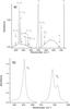 |
Fig. 1 Infrared spectrum of the methane ice at 15 K, before irradiation. In a) the absorbance scale has been enlarged to make the less intense combination bands of all CH4 assignments visible and b) zoom of the ν3 (this band is slightly saturated, but it does not significantly change the band profile) and ν4 assignments. The vibration modes at 1302 and 1298 cm-1 are considered as centered at 1300 cm-1. |
To place limits on the maximum ice thickness, the proportionality between the absorbance due to an intense band (3009 cm-1) and the 30 times weaker (4202 cm-1) was verified. The results presented in Fig. 2 show that our sample does not correspond to the saturation regime, therefore the Lambert-Beer law is applicable up to 3 μm thick CH4 ice.
The sample was irradiated by 220 MeV 16O7+ ions (i.e., v2 ~ 14 MeV/u ions) in a chamber at the medium energy beam line of the heavy ion accelerator GANIL (Grand Accélérateur National d’Ions Lourds). The beam impinged perpendicularly to the sample at constant beam flux 1 × 10⁹ ions/cm2s up to a final fluence of 4.29 × 10¹³ ions/cm2. A sweeping device assures a homogeneous irradiation of the sample surface. The stopping power of 220 MeV oxygen projectiles in CH4 is 76.5 × 10⁻¹⁵ eV/molecule/cm2 (SRIM) (Ziegler et al. 1985), and the total energy loss per projectile in the ice layer was about 206 keV. This amount is negligible with respect to initial energy. Therefore, cross sections do not change with ion penetration depth. Beyond the ice target, the beam was stopped in the 2 mm thick CsI substrate. The dose absorbed by the CH4 is estimated to be 3.3 eV per molecule at the end of irradiation.
3. Results
The effect of irradiation on CH4 is illustrated in Figs. 3a and b, where relevant sections of the FTIR spectra acquired before and after irradiation are compared.
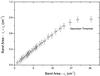 |
Fig. 2 Comparison between the increase of band areas corresponding to the (ν1+ν4) − 4202 and (ν3) − 3009 cm-1 transitions of CH4 during continuous ice deposition at 15 K. |
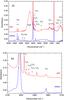 |
Fig. 3 Comparison of FTIR spectra regions of the CH4 ice at 15 K before (lower) and after (upper) irradiation. The spectrum corresponds to a final fluence of 4.29 × 10¹³ ions/cm2. a) Range of 600 − 5000 cm-1 and b) range of 2700 − 3100 cm-1. |
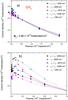 |
Fig. 4 a) Comparison of the CH4 column densities evolution obtained from the analysis of five IR transitions normalized to the band 4202 cm-1 at F = 1.0 × 10¹³ impacts/cm2. b) At lower fluences, there are differences among the column density absolute values, as discussed in Sect. 3.2.1 on the CH4 analysis. |
3.1. Identification of IR bands
Five CH4 IR absorptions bands can be identified: i) the fundamental deformation mode (ν4) centered at 1300 cm-1; ii) three vibrations combinations bands: (ν3 + ν4), 4300 cm-1, (ν1 + ν4) at 4202 cm-1 and another (ν2 + ν4) at 2815 cm-1; and iii) a second fundamental stretching peak (ν3) centered at 3009 cm-1. The CH4 column density dependence on beam fluence is presented in Fig. 4. The simultaneously analysis of five different bands may help for obtaining a correct column density value. Indeed this proposed procedure allow us to (i) examine possible saturation in the detector; (ii) check whether other species contribute to the analyzed peak; and/or (iii) observe possible phase transition. Moreover, the internal normalization provides consistency among A-values for the five bands in the column density calculation. From this analysis, the band 4202 cm-1 was selected as the reference feature (see Sect. 3.2.2).
In Table 1, the band position, assignments, and characterization of all the observed vibration modes of CH4 daughters are compared with those of the literature. A very small initial contamination of CO2 (ν3 − 2346 cm-1), CO (2138 cm-1), and H2O bands 3714 cm-1 and 3255 cm-1 (Ehrenfreund et al. 1996) are also observed.
Comparison of peak positions, assignments, and characterizations of CH4 daughter molecules at 220 MeV 16O+7, a fluence of 4.29 × 10¹⁹ ions/cm2.
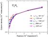 |
Fig. 5 Column density dependence of C2H6 daughters molecules on beam fluence. Solid lines are guides for the eyes. See Sect. 3.2.2 for further discussion of the dispersion observed at low fluences. |
3.2. Column density determination
The knowledge of the A-value is crucial for determining of the correct column density, as related in Eq. (1). The A-values available in the literature may not be adequate for a particular target, since these values may change with ice temperature and crystalline phase. Two tests should be considered in this analysis:
-
(i)
For a given molecular species, the consistency of the relativevalues of A due to its distinct bands can be checked by verifying that the same column density is obtained from the respective absorbance bands (see Figs. 4 and 5).
-
(ii)
For the precursor species and its daughter species, the consistency of their A relative values can be checked by the so-called carbon budget test (Bennett et al. 2006): if no sputtering of these species occurs, the total number of carbon atoms must stay constant during irradiation regardless of the chemical reactions induced by radiation.
Comparisons of the integral absorption coefficient A (10-18 cm molecule-1) used in the current work with those reported in literature for the CH4 and for its products formed by the heavy ion irradiation.
3.2.1. CH4 analysis
For the current CH4 data, the two tests revealed problems with the A-values found in the literature. To find coherent A-values, the column densities of all the others CH4 transitions were normalized to the band 4202 cm-1 over a high fluence region (F = 1.0 × 10¹³ ions/cm2), assuming that the A-value reported by (Brunetto et al. 2008) is the correct one. The normalized A-values obtained are displayed in the last column of Table 2.
The effect of this normalization is presented in Fig. 4a for the whole fluence range and in Fig. 4b for the low fluence region. It is observed that all the curves have the same slope at high fluence, showing that the corresponding column densities are proportional to that of the 4202 cm-1 band. In contrast, this is not the case for low fluence where data are scattered. There are different ways to express this finding: (i) the structure of ice is changing; (ii) the A-value for a virgin ice is not the same as for a high-fluence regime when the ice phase is already stable; and (iii) the relative variations in the A-value for distinct IR bands of the same molecular species are different from each other in the low-fluence region.
It follows from this analysis that the initial column density of CH4 measured by FTIR spectrum of the virgin ice (Nvirgin = 2.69 × 10¹⁸ molecules/cm2) is in good agreement inside the error bar, with N0 = 2.66 × 10¹⁸ molecules/cm2 obtained from extrapolating high-fluence data towards F = 0. It can be verified that the current normalized A-values are in fair agreement with the work of Brunetto et al. (2008), Mulas et al. (1998) (band 3009 cm-1), and Gerakines et al. (2005) (band 1300 cm-1). For the carbon budget calculation, we assume that the band at 4202 cm-1 (ν1 + ν4) is the adequate one, as described in Sect. 3.5.
3.2.2. Daughter species analysis
The A-values for the molecular species produced under irradiation of the CH4 ice are also displayed in Table 2. Data for them are scarce, so we adopted some of the available values in literature (Table 2). In the case of disagreement between two bands for the column density determination, normalization to a reference band at F = 1.0 × 10¹³ ions/cm2 was carried out, following the same procedure as for the CH4 analysis.
The appearance of the methyl radical CH3 is observed via its ν2 vibration at the top of intense band at 608 cm-1. For this band we adopted the A-value (25 × 10-18 cm molecule-1) previously reported by Gerakines et al. (1996), Moore & Hudson (2003), and Kaiser & Roessler (1998).
Four stable daughter species also appeared during irradiation: C2H2, C2H4, C2H6, and C3H8. Vibration modes of the C2H2 molecule at 736 cm-1 and 3267 cm-1 have been commonly attributed to the ν5 and ν3 vibration modes, therefore we assume the same A-value in the literature such as the A = 14 × 10-18 cm molecule-1 (Moore & Hudson 1998; Kaiser & Roessler 1998) and A = 32 × 10-18 cm molecule-1 (Kaiser & Roessler 1998), respectively. The molecule C2H4 is identified by the bands at 952 cm-1 and 3095 cm-1, which rise at the beginning of the irradiation. We also used for those bands the values available in literature such as A = 15 × 10-18 cm molecule-1 and 1.0 × 10⁻¹⁸ cm molecule-1 (Moore & Hudson 1998; Kaiser & Roessler 1998), respectively. For those bands, the A-values agree with each other, differing for the ν12 vibration mode at 1436 cm-1. The band 1436 cm-1 has been normalized to the band 952 cm-1 (see Table 2). For C3H8 vibration mode ν1 at a peak at 2962 cm-1, the attributed A-value was the only the available in the literature: 15.8 × 10⁻¹⁸ cm molecule-1 (Moore & Hudson 1998).
The C2H6 molecule is the most abundant daughter species formed; this molecule is identified through its ν12, ν11, ν6, ν5, and ν10 vibrations at 821 cm-1 (Kaiser & Roessler 1998), 1463 cm-1 (Moore & Hudson 1998; Kaiser & Roessler 1998), 1375 cm-1, 2884 cm-1, 2975 cm-1 (Kaiser & Roessler 1998), respectively. The A-values for C2H6 bands displayed in the last column of Table 2 were determined from the normalization to the band at fluence = 1.0 × 10¹³ ions/cm2. For this band (821 cm-1) we adopted the value A = 1.9 × 10⁻¹⁸ cm molecule-1 used by (Kaiser & Roessler 1998). For the carbon budget test, described in Sect. 3.4, we have adopted this band. From Fig. 5, it can be noticed that the shapes for all the vibration modes agree quite closely. The change in the interaction of newly formed C2H6 molecules with the surrounding environments (matrix effect) that is evolving, under irradiation, both structurally and chemically may the responsible for the absolute value dispersion observed at low fluences.
The C2H5 transition at band 534 cm-1 is out of range of the current FTIR spectrometer so could not been observed. The C2H3 peak at 893 cm-1 was not seen, and contributions from other species such as CH3OH and CH were not observed.
3.3. Water layering
Just before irradiation, the H2O column density in the ice bulk was 2.12 × 10¹⁵ molecules/cm2, measured from the peak at ~3200 cm-1. During the experiment, a thin ice water grew up continually onto the CH4 target to a final column density 5.38 × 10¹⁶ molecules/cm2 (~163 Å thickness). Figure 3a illustrates the increase in the water absorbance in the irradiated spectrum after about 12 h of irradiation by comparing with the virgin ice spectrum. If neglecting the water deposited during the FTIR acquisition (when the ion beam was stopped), these numbers correspond to a net deposition rate under irradiation of 1.21 × 10¹² H2O molecules/cm2 s, i.e., to a net deposition yield (the balance between the layering yield, L, and the sputtering yield, YS) of about L − YS = 1206 water molecules/projectile. Relevant comments on the water layering follow.
-
(i)
The water layer practically does not interfere on the projectileinteraction with CH4 in the bulk. Indeed, at the end of the irradiation, the water ice thickness has increased by 50 monolayers, which reduces the kinetic energy loss of the oxygen projectiles by only 2.2 keV.
-
(ii)
Chemical reactions may occur in the H2O–CH4 interface, producing hybrid species such as H2CO2 and CH3OH. However, the IR peaks of these species are not observed in the current experiment even after high fluence irradiation. Other hybrid species such as CO2 and CO can be formed at the interface. Although very small quantities of CO2 and CO were observed in the virgin CH4 ice, it should be noted in Fig. 3a that the amount of CO2 after irradiation is much higher than the initial impurities in the sample.
-
(iii)
The existence layer of H2O ice on top of the CH4 target drastically inhibits the CH4 sputtering: the emission energy of the sputtered species lies in the eV range (see e.g., Pereira 1997; Jalowy et al. 2004), so they are not expected to traverse even thin H2O layers. Actually this brings a convenient simplification to the analysis, since the sputtering contribution can be eliminated from the mathematical description, as shown in Eq. (2) by neglecting sputtering yield Yi.
Formation (σf) and destruction (σd) cross-sections, as well as the G of the CH4 and its daughters.
Summary of column density variation of the observed species: destruction and formation yields at the end, with a fluence of 4.29 × 10¹³ ions cm-2.
3.4. Cross section determination
Figure 6 shows the evolution of CH4 column density as a function of 220 MeV oxygen beam fluence. The decreasing CH4 column density is related to the formation of other species and to the sputtering induced by heavy ions (Seperuelo Duarte et al. 2009, 2010; Pilling et al. 2010). The behavior of these data is assumed to be described by the system of differential equations: 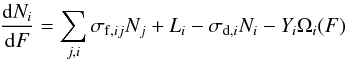 (2)where Ni is the column density of molecular species i, σf and σd are their formation and destruction cross sections, Li and Yi are their layering and sputtering yields respectively, and Ωi(F) is coverage of the species i on the surface after the beam fluences F.
Concerning the current experiment, these differential equations can be simplified and solved analytically under the following approximations:
-
(i)
The initial ice is formed by a single molecular species. Theprecursor molecule, CH4, is labeled i = 1.
-
(ii)
There is no layering of CH4 during irradiation (L1 = 0, but it does exist for water, an accumulative target surface contaminant as explained in Sect. 3.3).
-
(iii)
Sputtering is neglected for CH4 and for its products: Yi = 0, although at the beginning of irradiation the surface water layer is not thick enough to prevent completely the CH4 secondary emission. At any rate, the effect of sputtering on N1(F) would be more evident at high fluences owing to thickness reduction, which is not seen in the current data (Seperuelo Duarte et al. 2009, 2010).
-
(iv)
To obtain a solvable system of equations we have to make the assumption that the formation of a given daughter species (i = k) can be treated independently of the others; i.e., the projectile does not produce a daughter species from other pre formed daughter species: σf,ij ≈ 0, where i and j hold for two daughters. This is a reasonable assumption at the beginning of the radiation, when the column density of the daughter species is much lower than that of CH4, Ni ≪ N1.
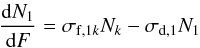 (3a)
(3a)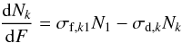 (3b)with the solutions
 ![Mathematical equation: % subequation 4090 0 \begin{eqnarray} \frac{N_1(F)}{N_1(0)}&=&\left[\frac{\sigma_{{\rm d},k}-\sigma_{{\rm d},1}}{\sigma_\Delta}\sinh\left(\frac{\sigma_\Delta F}{2}\right)+\cosh\left(\frac{\sigma_\Delta F}{2}\right)\right]\nonumber\\ && \times \, \exp\left(-\frac{(\sigma_{{\rm d},1}+\sigma_{{\rm d},k})F}{2}\right) \label{e5} \end{eqnarray}](/articles/aa/full_html/2011/07/aa16021-10/aa16021-10-eq132.png) (4a)
(4a)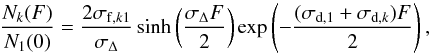 (4b)where
where σf,1k is the formation cross-section of CH4 from the k species. Inversely, σf,k1 is the formation cross-section of k species from CH4, and σd,1 is the destruction cross-section of CH4, whereas σd,k is the destruction cross-section of k species. The data were fitted by using the Eqs. (4). To obtain a formation cross section of CH4 (σf,1k), only the most abundant daughter species (C2H6) has been considered, and this value is reported as σf in the Table 3. It is worth noting that, for low fluences, Eq. (4b) can be expanded into
![Mathematical equation: % subequation 4090 3 \begin{equation} \frac{N_k(F)}{N_1(0)}\approx\sigma_{{\rm f},k1}\left[F-\frac{\sigma_{{\rm d},1}+\sigma_{{\rm d},k}}{2}F^2\right] \label{e8} \end{equation}](/articles/aa/full_html/2011/07/aa16021-10/aa16021-10-eq140.png) (4c)
(4c)
or transformed into
![Mathematical equation: % subequation 4090 4 \begin{equation} \frac{N_k(F)}{N_1(0)}\approx\sigma_{{\rm f},k1}\left[\frac{1-\exp[-(\sigma_{{\rm d},1}+\sigma_{{\rm d},k})F]} {[\sigma_{{\rm d},1}+\sigma_{{\rm d},k}]}\right]\cdot \label{e9} \end{equation}](/articles/aa/full_html/2011/07/aa16021-10/aa16021-10-eq141.png) (4d)
(4d)
Equation (4c) shows that the initial slope of the column density determines the formation cross section of the daughter molecules, while the curvature of the Nk(F) function depends on the precursor-daughter average dissociation cross section. Equation (4d) shows that Nk(F)/N1(0) ∝ (1 − exp(− σf,k1F)) or Nk(F)/N1(0) ∝ (1 − exp(− σd,kF)) are not the right functions for determining σf,k1 or σd,k from the fitting of the daughter’s data over a wide fluence range. Equations (4a) and (4b) were used to get the values of the destruction and formation cross sections of CH4 and their daughters, which are presented in Table 3. The evolution of column densities of the CH4 and of its most abundant daughters is shown in Fig. 6. The formation cross sections of each molecular species can be obtained from the slope of low fluences measurements, according to Eq. (4c), where σd,1 is kept constant for all fittings. This model is incomplete since it does not describe all chemical reactions, but does consider the k species as the unique daughter formed from the irradiated molecule, which is not generally the case. However, its predictions should be close to the exact one if the k species is the most abundant daughter. If many species are formed, then the sum of their formation cross sections should be equal to the destruction cross section of the precursor molecule, correcting for the chemical molecular balance. On the other hand, the relation between destruction cross sections of the daughters and the re-formation cross section of the precursor needs to take all the species concentrations into account. Table 3 presents the formation cross-sections and radiochemical yields (G-factors) for molecules identified in the present experiment. This factor allows comparison among chemical reaction yields produced by electrons, photons, and ions in the literature.
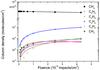 |
Fig. 6 Evolution of the column density of CH4 and the most abundant produced species. Solid curves are predictions given by Eqs. (4a) and (4b): the extracted cross sections are presented in Table 3. |
3.5. Carbon budget
The issue of the carbon budget is addressed by testing whether the column density of the methane destroyed can account for the column densities of the products. At the end of the irradiation we find that 3.87 × 10¹⁷ methane molecules were destroyed per square centimeter, which is about (14 ± 1)% of the original sample (Table 4). The total number of carbon atoms (per cm2) required to account for the observed column densities of the products at the end of the irradiation is obtained by adding each column density multiplied by the number of carbon in each species. Therefore for each one of the produced species we have CH3 = (5.71 ± 0.50) × 1015, C2H6 = (1.97 ± 0.50) × 1017, C2H4 = (1.82 ± 0.50) × 1016, C2H2 = (1.13 ± 0.50) × 1016, and C3H8 = (3.24 ± 0.50) × 1016. The total number of carbon required by the observed number of products is therefore 2.65 × 10¹⁷ carbon atoms cm-2, which corresponds to much fewer than produced by the methane destroyed.
Figure 7 shown the sum (line labeled with +) of the column densities of carbon atoms of the most abundant daughters species of the C2H2, C2H4, C2H6, CH3, and C3H8. Those values were multiplied by the number of carbon atoms in the corresponding molecule as a function of fluence. For a direct comparison with the CH4 molecules destroyed (full dots), the column N0 − NF is plotted. The column density variations of those species were estimated for a fluence of F = 4.29 × 10¹³ ion cm-2 (see Table 4). The destruction of CH4 gives 51% of C2H6, 8.4% of C3H8, 4.7% of C2H4, 2.9% of C2H2, and 1.5% of CH3, a total of 68.5%. Taking into account that no CH4 sputtering occurs in the current experiment, because of the water layer on the top of our CH4 ice, the rest of 31.5% of the destroyed CH4 can be related with some species which are not visible in our experiment. Possible candidates include C2, C2H3, C2H5, linear saturated and unsaturated hydrocarbons, as well as alkanes and polyclyclic aromatic hydrocarbons (PAHs) (Kaiser et al. 1992b,a). One important remark is that, if we choose the band 2975 cm-1 with the respective A-value from Gerakines et al. (1996) instead of the band 821 cm-1 adopted by Kaiser et al. (1996) and Bennett et al. (2006), the produced values C2H6 increase to (4.42 ± 0.50) × 1017, meaning that the destruction of CH4 is less than the creation of C2H6, and the carbon budget will not be conserved. This remark shows that the judicious choice of coherent A-values is important, because otherwise the abundance ratio may be incorrect, hence the formation cross section values. The column density calculation (or internal normalization) using different bands of the same transition is useful for minimizing this problem.
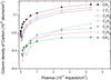 |
Fig. 7 Total and partial carbon column density as a function of beam fluence. The partial values are determined according to the carbon stoichiometry at the five most abundant species. The total value, which is the sum of all these curves, is labeled ΣCn and the column density of CH4 was plotted using the expression N0 − NF. |
Destruction of CH4 and formation of C2H6 molecules due to interaction with different projectiles inside a dense molecular cloud aged 100 Myr.
4. Astrophysical implications
It is interesting to compare the effects of methane ice irradiation by oxygen MeV ions with other ion irradiation sources such as UV photons, protons, α-particles, and electrons. The efficiencies of different irradiation sources for the destruction of the CH4 molecule and production of daughter species were calculated (the radiochemical yields – G-values). Data from previous works were digitized and the G-values were calculated taking the initial slopes of the column density curve as a function of the radiation dose. In present experiments for oxygen ions, G(CH4) = 5.0 molec (100 eV)-1, is nearly one order of magnitude more efficient for destroying methane than 7.3 MeV protons, 0.6 molec (100 eV)-1, or 9 MeV α-particles, 0.9 (100 eV)-1 (Kaiser & Roessler 1998). The values of G(CH4) = 2.8 molec (100 eV)-1, for irradiation with 30 keV He+, and 1.2 molec (100 eV)-1, for UV (10.2 eV photons), were estimated from Baratta et al. (2002). These results can be easily understood by considering the amount of energy transferred to the methane ices by each ion as given by the electronic stopping power: 76.5 (220 MeV O), 27.5 (30 keV α-particles), 20.3 (9.0 MeV α-particles), and 2.0 (7.3 MeV protons), in units of × 10-15 eV molec-1 cm2. It is important to note that 30 keV He+ ions are able to transfer an additional amount of 1.7 × 10⁻¹⁵ eV molec-1 cm2 due to nuclear stopping. We also estimated G(CH4) = 4.4 (100 eV)-1 for 5 keV electrons irradiation Bennett et al. (2006), which shows that they are as efficient as oxygen ions for destroying methane ice.
It is worth mentioning that G-values from daughter species can only be compared relatively, since they are greatly dependent on the A-values (and band) adopted. This is not the case for CH4, as long as absorbance is linearly related to the column density, which was assumed for all cases in the analysis above. In addition, Kaiser & Roessler (1998) and Bennett et al. (2006) used Reflection Absorption IR Spectroscopy (RAIRS) and A-values from transmission IR spectroscopy with no correction by “surface selection rule”. Therefore, absolute G-values should be compared with caution. For instance, G(C2H6) from Kaiser & Roessler (1998), 1.0 (100 eV)-1 (proton) and 1.3 (100 eV)-1 (α-particles), and Bennett et al. (2006), 4.0 (100 eV)-1 (electrons), are strikingly high in comparison with G(CH4). In the cases of both experiments from Kaiser & Roessler (1998), G(C2H6) are higher than G(CH4), which is impossible in principle. A relative comparison between G-values from daughter species shows subtle behavior on the efficiencies of form C2H4 and C2H2. The efficiency of forming C2H2 compared to C2H4 seems to increase with the energy (or mass) of the projectile. Electrons, on the other hand, seem to be very inefficient at forming C2H2 relative to C2H4.
The present results give information about the radiolysis occurring inside dense molecular clouds, where temperatures can be as low as 10 K and molecules condense on the surface of dust particles to form ice mantles. The densities of these clouds (~106 atoms/cm3) are high enough to prevent the penetration of UV photons deep inside them. However, ionization of atoms and molecules by cosmic rays within the cloud produce an internal UV radiation flux of 103 photons/cm2 s (Prasad & Tarafdar 1983). Energetic cosmic rays have higher penetration depths than UV photons and can trigger chemical reactions throughout an entire ice mantle.
We are now in a position to estimate how many CH4 and C2H6 molecules are destroyed and formed in a dense cloud during its typical life of 100 Myr. The flux of 220 MeV oxygen cosmic rays is (φ = 1.37 × 10⁻⁴ particles/cm2 s) (Shen et al. 2004). During a typical cloud’s life, 4.32 × 10¹¹ particles/cm2 penetrate the cloud. From the present work (Table 5) the number of CH4 destroyed for a 0.1 μm thick ice can be estimated as 2.2 × 10¹⁴ molecules/cm2, and a total of 6 × 10¹³ molecules/cm2 of C2H6 would be formed. The column density values are obtained by multiplying the yield values, normalized to 0.1 μm CH4 thick ice, by GCR fluence. Comparable results for other energetic particles are also included in this table. The values shown in Table 5 are far from completely describe the whole scenario. Other factors should be taken into account.
(i) In this work, only the results obtained for 220 MeV O, 7.3 MeV H and 9.0 MeV He beams are discussed. To determine the total number of destruction or formation of molecules in ISM by energetic particles from cosmic rays, it is necessary to integrate the contributions of all projectiles over their entire energy range. Therefore, more laboratory experiments should be performed to determine the cross sections as a function of projectile energy.
(ii) In the interstellar medium, the dust ice mantles are composed of mixtures of many different species. This complexity is obviously not described by Eqs. (4a) and (4b). Therefore, theoretical efforts are necessary to solve Eq. (2) for realistic cases.
5. Summary
The interaction of 220 MeV oxygen ions with pure CH4 ice has been studied. This projectile is one of the components of HGCR, and methane is a common molecule in the astrophysical environment. The results demonstrate that the MeV ion irradiation leads to production of CH3 and synthesis of C2H2, C2H4, C2H6, and C3H8. The destruction cross section of CH4 has been determined, as well as the formation cross sections of the observed daughters: CH3, C2H2, C2H4, C2H6, and C3H8. The most abundant daughter produced is C2H6. Concerning ion beams, oxygen is nearly one order of magnitude more efficient for destroying methane than protons or α particles. We emphasize that the A-values of precursor and daughter bands for estimating of column densities have to be consistently chosen in order to obtain reliable and correct formation cross section values and a valid carbon budget.
Acknowledgments
This work was supported by the region of “Basse-Normandie” (France) and by the French-Brazilian exchange program CAPES-COFECUB. It is a pleasure to thank Th. Been and J. M. Ramillon for technical support. The experiment was performed at the GANIL facility in Caen, France. We acknowledge the partial support of Brazilian agencies CNPq and FAPERJ.
References
- Baratta, G. A., Leto, G., & Palumbo, M. E. 2002, A&A, 384, 343 [NASA ADS] [CrossRef] [EDP Sciences] [Google Scholar]
- Bennett, C. J., Jamieson, C. S., Osamura, Y., & Kaiser, R. I. 2006, ApJ, 653, 792 [NASA ADS] [CrossRef] [Google Scholar]
- Bergin, E. A., Langer, W. D., & Goldsmith, P. F. 1995, ApJ, 441, 222 [NASA ADS] [CrossRef] [Google Scholar]
- Boogert, A. C. A., Schutte, W. A., Tielens, A. G. G. M., et al. 1996, A&A, 315, L377 [NASA ADS] [Google Scholar]
- Bringa, E. M., & Johnson, R. E. 2004, ApJ, 603, 159 [NASA ADS] [CrossRef] [Google Scholar]
- Brown, M. E., Bouchez, A. H., & Griffith, C. A. 2002, Nature, 420, 795 [NASA ADS] [CrossRef] [PubMed] [Google Scholar]
- Brown, M. E., Trujillo, C. A., & Rabinowitz, D. L. 2005, ApJ, 635, L97 [NASA ADS] [CrossRef] [Google Scholar]
- Brunetto, R., Caniglia, G., Baratta, G. A., & Palumbo, M. E. 2008, ApJ, 686, 1480 [NASA ADS] [CrossRef] [Google Scholar]
- Chapados, C., & Cabana, A. 1972, Can. J. Chem., 50, 3521 [NASA ADS] [CrossRef] [Google Scholar]
- Charnley, S. B., Rodgers, S. D., & Ehrenfreund, P. 2001, A&A, 378, 1024 [NASA ADS] [CrossRef] [EDP Sciences] [Google Scholar]
- Collado, V., Farenzena, L., Ponciano, C., Silveira, E., & Wien, K. 2004, Surf. Sci., 569, 149 [NASA ADS] [CrossRef] [Google Scholar]
- Cruikshank, D. P., Roush, T. L., Owen, T. C., et al. 1993, Science, 261, 742 [NASA ADS] [CrossRef] [PubMed] [Google Scholar]
- Ehrenfreund, P., Gerakines, P. A., Schutte, W. A., van Hemert, M. C., & van Dishoeck, E. F. 1996, A&A, 312, 263 [NASA ADS] [Google Scholar]
- Farenzena, L. S., Iza, P., Martinez, R., et al. 2005, Earth Moon and Planets, 97, 311 [Google Scholar]
- Gerakines, P. A., Schutte, W. A., & Ehrenfreund, P. 1996, A&A, 312, 289 [NASA ADS] [Google Scholar]
- Gerakines, P. A., Bray, J. J., Davis, A., & Richey, C. R. 2005, ApJ, 620, 1140 [NASA ADS] [CrossRef] [Google Scholar]
- Gibb, E. L., Whittet, D. C. B., Boogert, A. C. A., & Tielens, A. G. G. M. 2004, ApJS, 151, 35 [NASA ADS] [CrossRef] [PubMed] [Google Scholar]
- Griffith, C. A., Owen, T., Miller, G. A., & Geballe, T. 1998, Nature, 395, 575 [NASA ADS] [CrossRef] [PubMed] [Google Scholar]
- Hasegawa, T. I., & Herbst, E. 1993, MNRAS, 261, 83 [NASA ADS] [CrossRef] [Google Scholar]
- Jalowy, T., Farenzena, L. S., Ponciano, C. R., et al. 2004, Surface Science, 557, 91 [Google Scholar]
- Kaiser, R. I., & Roessler, K. 1998, ApJ, 503, 959 [NASA ADS] [CrossRef] [Google Scholar]
- Kaiser, R. I., Lauterwein, J., Müller, P., & Roessler, K. 1992a, Nucl. Instrum. Meth. Phys. Res. B, 65, 463 [NASA ADS] [CrossRef] [Google Scholar]
- Kaiser, R. I., Mahfouz, R. M., & Roessler, K. 1992b, Nucl. Instrum. Meth. Phys. Res. B, 65, 468 [NASA ADS] [CrossRef] [Google Scholar]
- Lacy, J. H., Carr, J. S., Evans, II, N. J., et al. 1991, ApJ, 376, 556 [NASA ADS] [CrossRef] [Google Scholar]
- Lanzerotti, L. J., Brown, W. L., & Marcantonio, K. J. 1987, ApJ, 313, 910 [NASA ADS] [CrossRef] [Google Scholar]
- Leger, A., Jura, M., & Omont, A. 1985, A&A, 144, 147 [NASA ADS] [Google Scholar]
- Licandro, J., Pinilla-Alonso, N., Pedani, M., et al. 2006, A&A, 445, L35 [NASA ADS] [CrossRef] [EDP Sciences] [Google Scholar]
- Lindal, G. F., Lyons, J. R., Sweetnam, D. N., Eshleman, V. R., & Hinson, D. P. 1987, J. Geophys. Res., 92, 14987 [NASA ADS] [CrossRef] [Google Scholar]
- Martinez, R., Ponciano, C., Farenzena, L., et al. 2006, Int. J. Mass Spectrom., 253, 112 [NASA ADS] [CrossRef] [Google Scholar]
- McKay, C. P., Martin, S. C., Griffith, C. A., & Keller, R. M. 1997, Icarus, 129, 498 [NASA ADS] [CrossRef] [PubMed] [Google Scholar]
- Moore, M. H., & Hudson, R. L. 1998, Icarus, 135, 518 [Google Scholar]
- Moore, M. H., & Hudson, R. L. 2003, Icarus, 161, 486 [NASA ADS] [CrossRef] [Google Scholar]
- Mulas, G., Baratta, G. A., Palumbo, M. E., & Strazzulla, G. 1998, A&A, 333, 1025 [NASA ADS] [Google Scholar]
- Nguyen, T. K., Ruffle, D. P., Herbst, E., & Williams, D. A. 2002, MNRAS, 329, 301 [NASA ADS] [CrossRef] [Google Scholar]
- Öberg, K. I., Fuchs, G. W., Awad, Z., et al. 2007, ApJ, 662, L23 [NASA ADS] [CrossRef] [Google Scholar]
- Öberg, K. I., Boogert, A. C. A., Pontoppidan, K. M., et al. 2008, ApJ, 678, 1032 [NASA ADS] [CrossRef] [Google Scholar]
- Öberg, K. I., van Dishoeck, E. F., & Linnartz, H. 2009, A&A, 496, 281 [NASA ADS] [CrossRef] [EDP Sciences] [Google Scholar]
- Owen, T. C., Roush, T. L., Cruikshank, D. P., et al. 1993, Science, 261, 745 [NASA ADS] [CrossRef] [PubMed] [Google Scholar]
- Pearl, J., Ngoh, M., Ospina, M., & Khanna, R. 1991, J. Geophys. Res., 96, 17477 [NASA ADS] [CrossRef] [Google Scholar]
- Pereira, J. 1997, Surf. Sci., 390, 158 [NASA ADS] [CrossRef] [Google Scholar]
- Pilling, S., Seperuelo Duarte, E., da Silveira, E. F., et al. 2010, A&A, 509, A87 [NASA ADS] [CrossRef] [EDP Sciences] [Google Scholar]
- Ponciano, C., Martinez, R., Farenzena, L., et al. 2006, J. Am. Soc. Mass Spectrom., 17, 1120 [Google Scholar]
- Prasad, S. S., & Tarafdar, S. P. 1983, ApJ, 267, 603 [NASA ADS] [CrossRef] [Google Scholar]
- Seperuelo Duarte, E., Boduch, P., Rothard, H., et al. 2009, A&A, 502, 599 [NASA ADS] [CrossRef] [EDP Sciences] [Google Scholar]
- Seperuelo Duarte, E., Domaracka, A., Boduch, P., et al. 2010, A&A, 512, A71 [NASA ADS] [CrossRef] [EDP Sciences] [Google Scholar]
- Shematovich, V. I., Shustov, B. M., & Wiebe, D. S. 1997, MNRAS, 292, 601 [NASA ADS] [Google Scholar]
- Shen, C. J., Greenberg, J. M., Schutte, W. A., & van Dishoeck, E. F. 2004, A&A, 415, 203 [NASA ADS] [CrossRef] [EDP Sciences] [Google Scholar]
- Smith, B. A., Soderblom, L. A., Banfield, D., et al. 1989, Science, 246, 1422 [NASA ADS] [CrossRef] [PubMed] [Google Scholar]
- Willacy, K., & Millar, T. J. 1998, MNRAS, 298, 562 [NASA ADS] [CrossRef] [Google Scholar]
- Willacy, K., & Williams, D. A. 1993, MNRAS, 260, 635 [NASA ADS] [Google Scholar]
- Ziegler, J. F., Biersack, J. P., & Littmark, U. 1985, The Stopping and Range of Ions in Solids (New York: Permagon) [Google Scholar]
All Tables
Comparison of peak positions, assignments, and characterizations of CH4 daughter molecules at 220 MeV 16O+7, a fluence of 4.29 × 10¹⁹ ions/cm2.
Comparisons of the integral absorption coefficient A (10-18 cm molecule-1) used in the current work with those reported in literature for the CH4 and for its products formed by the heavy ion irradiation.
Formation (σf) and destruction (σd) cross-sections, as well as the G of the CH4 and its daughters.
Summary of column density variation of the observed species: destruction and formation yields at the end, with a fluence of 4.29 × 10¹³ ions cm-2.
Destruction of CH4 and formation of C2H6 molecules due to interaction with different projectiles inside a dense molecular cloud aged 100 Myr.
All Figures
|
Fig. 1 Infrared spectrum of the methane ice at 15 K, before irradiation. In a) the absorbance scale has been enlarged to make the less intense combination bands of all CH4 assignments visible and b) zoom of the ν3 (this band is slightly saturated, but it does not significantly change the band profile) and ν4 assignments. The vibration modes at 1302 and 1298 cm-1 are considered as centered at 1300 cm-1. |
| In the text | |
|
Fig. 2 Comparison between the increase of band areas corresponding to the (ν1+ν4) − 4202 and (ν3) − 3009 cm-1 transitions of CH4 during continuous ice deposition at 15 K. |
| In the text | |
|
Fig. 3 Comparison of FTIR spectra regions of the CH4 ice at 15 K before (lower) and after (upper) irradiation. The spectrum corresponds to a final fluence of 4.29 × 10¹³ ions/cm2. a) Range of 600 − 5000 cm-1 and b) range of 2700 − 3100 cm-1. |
| In the text | |
|
Fig. 4 a) Comparison of the CH4 column densities evolution obtained from the analysis of five IR transitions normalized to the band 4202 cm-1 at F = 1.0 × 10¹³ impacts/cm2. b) At lower fluences, there are differences among the column density absolute values, as discussed in Sect. 3.2.1 on the CH4 analysis. |
| In the text | |
|
Fig. 5 Column density dependence of C2H6 daughters molecules on beam fluence. Solid lines are guides for the eyes. See Sect. 3.2.2 for further discussion of the dispersion observed at low fluences. |
| In the text | |
|
Fig. 6 Evolution of the column density of CH4 and the most abundant produced species. Solid curves are predictions given by Eqs. (4a) and (4b): the extracted cross sections are presented in Table 3. |
| In the text | |
|
Fig. 7 Total and partial carbon column density as a function of beam fluence. The partial values are determined according to the carbon stoichiometry at the five most abundant species. The total value, which is the sum of all these curves, is labeled ΣCn and the column density of CH4 was plotted using the expression N0 − NF. |
| In the text | |
Current usage metrics show cumulative count of Article Views (full-text article views including HTML views, PDF and ePub downloads, according to the available data) and Abstracts Views on Vision4Press platform.
Data correspond to usage on the plateform after 2015. The current usage metrics is available 48-96 hours after online publication and is updated daily on week days.
Initial download of the metrics may take a while.