| Issue |
A&A
Volume 530, June 2011
|
|
|---|---|---|
| Article Number | A14 | |
| Number of page(s) | 10 | |
| Section | The Sun | |
| DOI | https://doi.org/10.1051/0004-6361/201016096 | |
| Published online | 27 April 2011 | |
Asymmetries of the Stokes V profiles observed by HINODE SOT/SP in the quiet Sun
1
ESA/ESTEC RSSD, Keplerlaan 1,
2200 AG
Noordwijk,
The Netherlands
e-mail: This email address is being protected from spambots. You need JavaScript enabled to view it.
2
Dipartimento di Fisica, Università degli Studi di Roma “Tor
Vergata”, via della Ricerca
Scientifica 1, 00133
Rome,
Italy
3
Instituto de Astrofísica de Canarias, 38205 La Laguna, Tenerife, Spain
e-mail: This email address is being protected from spambots. You need JavaScript enabled to view it.
Received:
8
November
2010
Accepted:
18
March
2011
Abstract
Aims. A recent analysis of polarization measurements of HINODE SOT/SP in the quiet Sun pointed out very complex shapes of Stokes V profiles. Here we present the first classification of the SOT/SP circular polarization measurements with the aim of highlighting exhaustively the whole variety of Stokes V shapes emerging from the quiet Sun.
Methods. k-means is used to classify HINODE SOT/SP Stokes V profiles observed in the quiet Sun network and internetwork (IN). We analyze a 302 × 162 arcsec2 field-of-view (FOV) that can be considered a complete sample of quiet Sun measurements performed at the disk center with 0.32 arcsec angular resolution and 10-3 polarimetric sensitivity. This classification allows us to divide the whole dataset into classes, with each class represented by a cluster profile, i.e., the average of the profiles in the class.
Results. The set of 35 cluster profiles derived from the analysis completely characterizes the SOT/SP quiet Sun measurements. The separation between network and IN profile shapes is evident – classes in the network are not present in the IN, and vice versa. Asymmetric profiles are approximately 93% of the total number of profiles. Among these, about 34% of the profiles are strongly asymmetric, and they can be divided into three families: blue-lobe, red-lobe, and Q-like profiles. The blue-lobe profiles tend to be associated with upflows (granules), whereas the red-lobe and Q-like ones appear in downflows (intergranular lanes).
Conclusions. These profiles need to be interpreted considering model atmospheres different from a uniformly magnetized Milne-Eddington (ME) atmosphere, i.e., characterized by gradients and/or discontinuities in the magnetic field and velocity along the line-of-sight (LOS). We propose the use of cluster profiles as a standard archive to test inversion codes, and to check the validity and/or completeness of synthetic profiles produced by MHD simulations.
Key words: Sun: surface magnetism / Sun: magnetic topology / techniques: polarimetric / methods: statistical
© ESO, 2011
1. Introduction
The Stokes parameters (I, Q, U, and V) provide the main tool to analyze the solar photosphere. They are indeed molded by the photospheric structure and for this reason can tell us about its thermal, magnetic and dynamical properties.
When considering Stokes profiles measured in spectral lines that are sensible to magnetic fields via Zeeman effect, one could expect the circular polarization profiles (V) to be exactly antisymmetric with respect to a central wavelength of the transition, possibly shifted by plasma dynamics1. Contrary to such an idealization, the Stokes V profiles emerging from the solar photosphere present important asymmetries independently of whether the measurements are obtained with low spatial resolution (e.g., in plage or network regions; for a review see Solanki 1993) or with high spatial resolution (e.g., Sigwarth et al. 1999; Sánchez Almeida & Lites 2000; Domínguez Cerdeña et al. 2006; Viticchié et al. 2011), and both in network and in the interior of the network (IN).
Stokes V profile asymmetries are well known to be generated by gradients along and across the LOS of both magnetic field and plasma dynamics. Moreover, to deal with strong asymmetries one cannot consider mild variations of the above cited quantities, instead fairly large changes like discontinuities have to be invoked (e.g., Grossmann-Doerth et al. 2000). Discontinuities in model atmospheres can be produced in many different ways. They are found in canopy models (e.g. Grossmann-Doerth et al. 1988; Steiner 2000) or in embedded flux tube models (e.g., Solanki & Montavon 1993), in which one or two magnetopauses are present, i.e., sharp transitions from a magnetized region to a field-free one. Besides these models, one can consider the presence of many discontinuities along the LOS in solar magnetic fields as being intermittent over scales smaller than the photon mean free path at the photosphere (≃ 100 km); these are the MIcro-Structured Magnetized Atmospheres (MISMAs, Sánchez Almeida et al. 1996; Sánchez Almeida 1998). Smooth variations of the atmospheric properties can also be invoked, but large asymmetries require steep gradients in these continuous variations (e.g., Solanki & Pahlke 1988; Sánchez Almeida et al. 1988). The asymmetries are also partly caused by discontinuities across the LOS, in other words, an important factor which can introduce asymmetries is the finite spatial resolution of observations. The way it works remains unclear because rather than decreasing the asymmetries with improving angular resolution, the asymmetries observed in the quiet Sun with 0.32 arcsec seem to be more extreme than those obtained with 1 arcsec (cf. Sánchez Almeida & Lites 2000; Viticchié et al. 2011). On the one hand, one could expect to observe asymmetries mainly caused by gradients along the LOS when increasing the spatial resolution of the observations. On the other hand, we still do not know over which scale the magnetic field changes in the solar photosphere, e.g., in Vögler & Schüssler (2007) the magnetic field changes over approximately 10 km, well below the spatial resolution of HINODE.
The arguments considered above must be taken into account when interpreting Stokes measurements through inversion codes (e.g., Socas-Navarro 2001). Among these, the ones based on ME hypotheses cannot deal with asymmetries, but are still very important since they allow us to perform fast analyses of large datasets (e.g., Skumanich & Lites 1987; Orozco Suárez & Del Toro Iniesta 2007; Orozco Suárez et al. 2007a). On the other hand, several inversion codes that can fit and interpret asymmetric profiles are available. The MISMA inversion code (based on MISMA hypotheses, Sánchez Almeida 1997) has been successfully used to interpret strong asymmetries in polarization profiles emerging from the quiet Sun (Sánchez Almeida & Lites 2000; Domínguez Cerdeña et al. 2006; Viticchié et al. 2011). Other suitable tools to interpret Stokes V asymmetries are the SIR code (Ruiz Cobo & del Toro Iniesta 1992), or the SIRJUMP code (a modified version of the SIRGAUSS code, see Bellot Rubio 2003), which was already used for the interpretation of HINODE data (Louis et al. 2009).
Since its launch in 2006, the spectropolarimeter SOT/SP (Lites et al. 2001; Tsuneta et al. 2008) of the Japanese mission HINODE (Kosugi et al. 2007) allows the solar community to perform spectropolarimetry of the solar photosphere under extremely stable conditions. SOT/SP provides 0.32 arcsec angular resolution measurements with 10-3 polarimetric sensitivity. Moreover, its wavelength sampling (2.15 pm pixel-1) is suitable to have a detailed sampling of the polarization profiles. Many inversion analyses of spectropolarimetry measurements performed by SOT/SP have been performed so far. In most cases the hypothesis of ME atmosphere has been adopted (e.g., Orozco Suárez et al. 2007b; Asensio Ramos 2009; Ishikawa & Tsuneta 2009). Recently, Viticchié et al. (2011) provided the first interpretation of Stokes profile asymmetries revealed in the dataset analyzed by Orozco Suárez et al. (2007b) and Asensio Ramos (2009); the analysis was performed under MISMA hypotheses.
The aim of this paper is to further point out and quantify the complexity of the shapes of SOT/SP measurements already discussed in Viticchié et al. (2011), but using a tool independent of any inversion. To do this, we adopt a method that allows us to extract and characterize the typical shapes of the Stokes V profiles observed by SOT/SP in the quiet Sun. As will be emphasized in Sect. 4, a large part of these turned out to be strongly asymmetric. The main implication of this result is that refined inversion techniques should be considered in future analyses of SOT/SP data to extract further information on the structure of the solar photosphere. Those techniques are too burdensome to be viable for large datasets, but both the profile classes and families we present provide a small, yet complete set that is suitable for detailed study.
The paper is organized as follows: we introduce the dataset selected for the analysis in Sect. 2; we describe the classification tool adopted to extract the typical shapes of the Stokes V profiles from the dataset in Sect. 3; the typical profile shapes are presented in Sect. 4; we consider possible physical scenarios that could explain these profiles in Sect. 5, and reflect on further applications of the classes; finally, our conclusions are outlined in Sect. 6.
2. Dataset
We analyzed Stokes I and V profiles of a 302 × 162 arcsec2 portion of the solar photosphere observed at disk center on 2007 March 10 between 11:37 and 14:34 UT. The spectropolarimetric measurements were taken by the SOT/SP instrument aboard HINODE (Lites et al. 2001; Tsuneta et al. 2008) in the two Fe i 630 nm lines, with a wavelength sampling of 2.15 pm pixel-1, and a spatial sampling of 0.1476 arcsec pixel-1 and 0.1585 arcsec pixel-1 along the east-west and south-north directions, respectively. The data reduction and calibration were performed using the sp_prep.pro routine available in the SolarSoft (Ichimoto et al. 2008). After correction for the gravitational redshift, we verified that the cores of the full-FOV average Stokes I profiles coincide within the SOT/SP wavelength sampling with the cores of the two Fe I lines in the Neckel atlas (Neckel 1999). Moreover, the average line cores vary across the scanning direction with a standard deviation of approximately 60 m s-1, discarding the problem mentioned by Socas-Navarro (2011). This accuracy of the absolute wavelength scale suffices because we mostly use relative velocities, and the absolute scale is employed only to distinguish granules and intergranules (i.e., upflows and downflows). Using the polarization signals in continuum wavelengths, we estimated a noise level of σV ≃ 1.1 × 10⁻³ Ic for Stokes V (Ic stands for the average continuum intensity of the FOV). The dataset has been already analyzed by Orozco Suárez et al. (2007a), Lites et al. (2008), Asensio Ramos (2009), and Viticchié et al. (2011) to derive the magnetic properties of IN and network regions. Consistently with these works, here we focus on Stokes V profiles whose maximum amplitude is larger than 4.5 × σV. A total of 535 465 Stokes V profiles meet the selection criteria (i.e., 26% of the total number of profiles in the dataset). Such a large number of profiles can be rightly considered a complete set of polarization signals representative of the different Stokes V profiles that can be observed in the quiet Sun at disk center with 0.32 arcsec resolution and 10-3 polarimetric sensitivity.
3. Data analysis
The analysis consists of three main parts. The most important one is the k-means classification of the profiles. This allows us to infer the typical profile shapes from the dataset described in Sect. 2. Besides the classification, we derived the LOS velocity for each pixel in the FOV adopting a Fourier transform method applied to both Stokes I lines separately (Title & Tarbell 1975), and the center-of-gravity magnetogram signal from Stokes I and V (COG, Rees & Semel 1979).
The k-means classification algorithm is commonly used in data mining, machine learning, and artificial intelligence (e.g., Everitt 1995; Bishop 2006). Indeed, the procedure we use is the same as the one used by Sánchez Almeida et al. (2010) to analyze galaxy spectra from the Sloan Digital Survey Data Release 7. In this work the authors defined the procedure as automatic and unsupervised. “Unsupervised” implies that the algorithm does not have to be trained, whereas “automatic” means that it is self-contained, with minimal subjective influence. In the standard formulation, k-means begins by selecting at random from the full dataset of V spectra a number k of template spectra. Each template spectrum is assumed to be the center of a cluster, and each spectrum of the data set is assigned to the closest cluster center (i.e., that of minimum distance or, equivalently, closest in a least-squares sense). Once all spectra in the dataset were classified, the cluster center is re-computed as the average of the spectra in the cluster. This procedure is iterated with the new cluster centers, and it finishes when no spectrum is re-classified in two consecutive steps. The number of clusters k is arbitrarily chosen but, in practice, the results are insensitive to this selection because only a few clusters possess a significant number of members, so that the rest can be discarded. On exit, the algorithm provides a number of clusters, their corresponding cluster centers, as well as the classification of all the original spectra now assigned to one of the clusters. The classes are ordered according to the total number of profiles they contain, i.e., assigning 0 to the most abundant, 1 to the second most abundant, and so on.
As a major drawback, k-means yields different clusters with each random initialization, therefore, one has to study this dependence by carrying out different random initializations and comparing their results. Partly trying to alleviate this problem, the code we employ uses an initialization more refined than the plain random initialization. It consists of four steps: (Step 1) choose at random ten initial cluster centers; (Step 2) run one iteration of the standard k-means, and select as initial cluster center the cluster center with the largest number of elements; (Step 3) remove from the set of profiles to be classified those belonging to the cluster center thus selected; (Step 4) go to step 1 if profiles are still left; otherwise end. In order to show that the method is working properly, in Sect. 4 we present the results obtained from a single classification run and then validate them by showing that they fully agree with the average results obtained when performing ten classification runs initialized with different random conditions.
An important point to be mentioned is that the classes provided by k-means do not form an orthogonal basis in the principal component analysis sense (e.g. Connolly et al. 1995; Rees et al. 2000). The individual profiles are not unique linear superpositions of the cluster center profiles. Indeed, among the clusters found by the analysis, similar profiles can be easily recognized (Fig. 1). However, it is important to specify that the aim of our classification is not to provide orthogonal classes, but to point out the typical shapes of the profiles observed by SOT/SP in the quiet Sun. The most important point to keep in mind is that all profiles associated to a given class are similar to the cluster profile representative of the class and, therefore, the cluster profiles are effectively representative of the shapes of the profiles observed by SOT/SP. Referring to the similarity between each cluster profile and the profiles associated to it, it is worth pointing out that profiles strongly deviating from the cluster center are discarded. In more detail, when the cluster centers are calculated as the average of the profiles in the class, those members with a distance larger than three times the standard deviation are rejected.
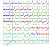 |
Fig. 1 Classes of Stokes V profiles of Fe i 630.15 nm (left) and Fe i 630.25 nm (right) in the quiet Sun according to a single k-means classification run. All the classes retrieved by the analysis are reported. Each panel contains the average (solid lines) and the standard deviation (colored error bars) of all profiles in the class. The dotted vertical line separates the two spectral lines (it divides the x-axis in two windows of 40 pixels, see Sect. 3.1). Each plot is represented in the same x − y range, i.e., the one of class 30. The number of the class is specified in each plot together with the percentages of profiles in the class. The colors group classes in families of alike profiles (Sect. 4): network (purple), blue-lobe (blue), red-lobe (red), Q-like (sky-blue), asymmetric (green), antisymmetric (yellow), and fake (orange). |
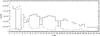 |
Fig. 2 Histograms with the number of pixels in each class considering network regions (purple dot-dashed line) and IN regions (black solid line) separately. The arrows point out the network classes as derived from the statistics. |
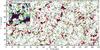 |
Fig. 3 Spatial distribution of the profile families. Each color is representative of a single family according to the color code in Fig. 1. White pixels are the ones with max(| V|) < 4.5 × σV, which are excluded from the classification analysis. Red contours highlight the network regions in the FOV. The inset contains a 15 × 15 Mm2 detail of the FOV (black square) for a better visualization of the small family patches around a network region. The black contours highlight the regions with continuum intensity above the average continuum intensity of the FOV, i.e., the granules. |
3.1. Definition of the input dataset archive
Given a set of observations, the actual data to be classified can be chosen in different ways (e.g., range of wavelengths to be included, or whether the profiles are corrected for the magnetic polarity). Here we explain the way our dataset was defined and why.
The main idea is to analyze exclusively the shape of Stokes V. For this reason we remove the global shift of the profiles, renormalize each profile to its maximum unsigned value, and sign the profiles according to the main polarity in the resolution element.
Each profile is normalized to its maximum absolute amplitude as  (1)where λ spans over the whole wavelength range of SOT/SP (i.e., 0.24 nm around 630.2 nm).
Global wavelength shifts are removed separately for the two spectral lines. We extract the Stokes V profiles of the two Fe i lines in two wavelength windows that are centered around the corresponding Stokes I line cores. The two wavelength windows have the same amplitude, i.e. 86 pm, so that both lines contribute to the classification with the same number of wavelength pixels. In this procedure the number of wavelength pixels is reduced from 112 to 80 (i.e., two windows of 40 wavelength pixels each). It is important to keep in mind that after this step it is not possible to consider a common wavelength range for the representation of Stokes V profiles of the two lines. For this reason, the abscissas of our Stokes V profiles are given in pixel units rather than wavelengths (see Fig. 1).
Finally, we individually sign the profiles according to the polarity that dominates Stokes V, so that if V were perfectly antisymmetric, the polarity-corrected Stokes V would have a positive blue lobe and a negative red lobe. Since the signals are not antisymmetric, we define dominant polarity as that yielding a V with the sign of the largest average signal in the profile. In practice, we average Stokes V separately in the red-wing and the blue-wing to decide which wing dominates. The division between red and blue is set by the Stokes I line core wavelengths. If the (unsigned) blue-wing signal is largest, then we divide Stokes V by its sign. If the (unsigned) red-wing signal is largest, then we divide Stokes V by minus its sign. The result is a V profile with the largest signal positive if it happens in the blue-wing, and negative if happens in the red-wing (see the profiles in Fig. 1 for illustration).
4. Results
The main result of the k-means classification is reported in Fig. 1. It shows the cluster centers for all classes of profiles existing in the quiet Sun. After several trial classifications, we set the maximum number of allowed classes to 50, which exceeds the typical number of classes retrieved by the procedure (i.e., around 35, see Table 1). In this way we are sure that the classification procedure is automatically setting the number of classes. The classification performed on the dataset of 535 465 profiles took about 20 min on a standard laptop.
We number the classes according to the percentage of observed profiles belonging to the class, from the most common, class 0, to the least common, class 34. It is important to notice that strongly asymmetric profiles are found throughout, e.g., the second most populated class shows important asymmetries. Classes of Stokes V with three lobes (Q-like profiles) are also common, meaning that profiles like this are not isolated cases in quiet Sun measurements.
As already reported in Sect. 3, similar profile shapes can be recognized among the cluster profiles in Fig. 1. Indeed, attending to their basic properties the profiles can be grouped in six families: network, blue-lobe, red-lobe, Q-like, asymmetric, and antisymmetric (partially following Steiner 2000). With basic properties we refer to the major features of profiles, e.g., blue-lobe profiles have a very small red lobe so that, independently of the amount of polarization in the blue lobe, they are dominated by the blue lobe itself.
The first family, i.e., the network one, can be defined by calculating the statistics for the k-means classes when network and IN regions are considered separately, i.e., for the pixels included/not-included in the red contours of Fig. 3. The contours separate network and IN regions in the FOV. Network patches were identified with the algorithm used in Viticchié et al. (2011). We refer to this work for details, but it basically selects the patches with the largest polarization signals that all together cover some 10% of the FOV2. The statistics is reported in Fig. 2, here the network classes are pointed out by arrows. More in detail, the network-IN division performed by the routine has an equivalent division in the k-means classes. Indeed, the classes that are abundant in the network (i.e., those pointed out by the arrows) are scarce in the IN, and vice-versa3. These results imply that the network is associated with particular Stokes V shapes that are not found elsewhere. In other words, a classical network identification and the k-means classification point out the same regions with two different methods: the first one is mainly based on the analysis of the spatial coherence of strong Stokes V signals, whereas the second one does not take into account the amplitude of Stokes V (profiles are normalized before classification, see Sect. 3.1), and refers just to profile shapes. The “network family” contains the following group of k-means classes: classes 0, 3, 4, 6, 7, 12, and 19 (the cluster profiles of these classes are reported in Fig. 1 with purple error bars). These are representative of about 28.6% of the total number of analyzed pixels. By examining the shapes of the clusters in the network family one can notice that these profiles present the blue lobe larger than the red one, while the latter is more extended in wavelength (its area is larger than the area of the blue lobe). Such a shape is well known to be associated to network regions (e.g., Stenflo et al. 1984; Sánchez Almeida et al. 1996). Moreover, the amplitude of the Stokes V profiles in the two lines is very similar in all network classes; this highlights the fact that a saturation due to kG fields is present, as expected in network regions (see, e.g., Socas-Navarro & Sánchez Almeida 2002; Stenflo 2010). As explained above, each profile emerging from HINODE pixels with sufficient signal is associated to a class and, by grouping of classes through a certain criteria, to a family. In Fig. 3 we identify the position of a network profile with a purple pixel. The map shows how the network contours highlight large purple patches.
On the other hand, clusters profiles in IN pixels present a huge variety of asymmetries. As an example, class 1, the most abundant class in the IN, is represented by a cluster profile dominated by the blue lobe. Many other classes are represented by profiles dominated by a single lobe, either the blue one or the red one (here always negative because of the condition imposed in Sect. 3.1). The profiles in these classes represent approximately 34.4% of the analyzed pixels. Among these, 17.5% are the profiles dominated by the blue lobe, named the “blue-lobe family”, i.e., class 1, 5, 10, 15, and 28 (represented with blue error bars in Fig. 1 and blue pixels in Fig. 3) and 9.6% by the red lobe, named the “red-lobe family”, i.e., 17, 21, 23, and 24 (represented with red error bars in Fig. 1 and red pixels in Fig. 3). Moreover, a third family of extremely asymmetric profiles can be defined; class 25, 26, 30, 31, 33, and 34 (represented with sky-blue error bars in Fig. 1 and sky-blue pixels in Fig. 3) form the “Q-like family”, which contains 7.3% of the total number of analyzed pixels.
The classes still not considered are IN profiles presenting shapes that are not clearly among the three families defined above. In spite of this, many of these profiles still present evident asymmetries; the “asymmetric family” is formed by the class 2, 8, 11, 13, 14, 16, 18, 22, 27, and 32 which are 29.6% of the analyzed profiles (represented with green error bars in Fig. 1 and green pixels in Fig. 3). Finally, only two classes show almost antisymmetric profiles; these represent only 6.3% of the dataset (i.e., class 9 and 20) and are named the “antisymmetric family” (represented with yellow error bars in Fig. 1 and yellow pixels in Fig. 3).
Another interesting result comes from the study of the position of the families on the FOV. This can be done, for example, by studying the LOS velocity (vlos) for the pixels associated to each family. Pixels with vlos < 0 (vlos > 0) are placed in granules (intergranular lanes), i.e., upflow regions (downflow regions). Figure 4 contains the result of such a study when calculating the statistics of vlos (as derived by Stokes I, see Sect. 3) for the pixels included in the six families defined above. The main result derived from this study is that each family is related to a certain dynamics. This is very revealing because the classification procedure does not know anything about vlos because wavelength shifts were removed when extracting Stokes V profiles in the wavelength windows centered around Stokes I cores (Sect. 3.1). From this one learns that the plasma dynamics, as derived from Stokes I, i.e., the dynamics mostly associated to the non magnetized plasma in the pixel, is in some way related the shape of Stokes V profiles. One can elaborate a bit more on this result. The separation between the families with one lobe only (i.e., the blue-lobe and the red-lobe) is evident. On the one hand, profiles dominated by the blue lobe are mostly found in upflow regions, i.e., on top of the granules. On the other hand, profiles dominated by the red lobe are mostly found in downflow regions, i.e., intergranular lanes. The Q-like, network, and asymmetric families are found in downflow regions. Antisymmetric profiles are found in both upflow and downflow pixels with almost the same probability. Overall, as expected, most of the polarization signals reside in downflows, i.e., 68.3% of the analyzed pixels.
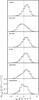 |
Fig. 4 Statistics of the LOS velocities (vlos) of the pixels associated with each family of Stokes V shapes. Each plot contains the histograms of the vlos derived from both Fe i 630.15 nm (thick lines) and Fe i 630.25 nm (thin lines). The histograms are normalized to the total number of profiles in the family. The vertical dotted lines separate the upflow regime (left) and the downflow regime (right). |
Different families are also associated with different spatial extents. When calculating the area of the largest patch4 in the FOV formed, exclusively, by profiles of the particular family one finds that network patches, mainly associated with class 3 and 4, can reach dimensions up to few tens arcsec2. All other families have typical patch dimensions of few tenths of 1 arcsec2 (see for a comparison the detail image in Fig. 3 in which contours highlighting the granular scale are reported). This means that out of network regions the profile shape of the analyzed profiles change over very small scales, smaller than the typical granular scale.
The results presented in this section were derived from a single k-means classification run. As specified in Sect. 3 it is important to study the dependence of the results on different random initializations. To do this, we derived the average abundances of the different families from ten classification runs; Table 1 allows one to compare the average results with those presented above. From this we can conclude that the results presented are sound and that the classification does not depend on the random initialization.
The only class we did not consider so far in the presentation of the results is class 29, representative of 1.1% of the analyzed profiles. This can be considered a fake class since it contains anomalous profiles. Here we define as anomalous, for example, those profiles on which the procedure adopted for the definition of the input dataset (Sect. 3.1) did not work properly. A single fake class is found in all classification runs; this is always representative of about 1% of the analyzed profiles. This can be verified also in Table 1, indeed by adding up the percentages from all families one gets 99% of the analyzed profiles.
5. Discussion
An important point to emphasize is that the number of k-means classes representative of all the profiles observed by SOT/SP (35 ± 3) is small compared to the total number of profiles in the analyzed dataset (535 465). Moreover, when the major features of the classes are considered, the analyzed profiles can be organized in six families (i.e., network, blue-lobe, red-lobe, Q-like, asymmetric, and antisymmetric) so that a few shape typologies can represent SOT/SP quiet Sun data. Nevertheless, it is important to note that almost all these shapes are strongly asymmetric.
Most SOT/SP data have been so far interpreted through ME codes (Orozco Suárez et al. 2007a; Asensio Ramos 2009), but the k-means classes in Fig. 1 show that such an hypothesis has to be replaced to analyze the whole variety of profile shapes observed by SOT/SP in the quiet Sun. Except for the classes whose profile shapes can be reasonably considered to be quasi-antisymmetric (see Sect. 4), we can conclude that ME codes cannot reproduce the observed profiles observed by SOT/SP. Orozco Suárez et al. (2010) recently showed that ME codes can be used to derive average properties of fully resolved magnetized atmospheres (technically speaking with magnetic filling factors equal to 1) even when inverting extremely asymmetric profiles. This good news does not eliminate the need for more refined inversions. The asymmetries provide information on the unresolved structure and/or gradients along the LOS of the magnetic field that are washed out unless the line shapes are adequately interpreted. Moreover, the present angular resolutions do not grant treating all IN magnetic features as fully resolved.
These considerations can be used in a constructive way when thinking about future strategies for the interpretation of spectropolarimetric data either from HINODE or from future telescopes. One needs different hypotheses in order to interpret (and fit) the different polarization profiles emerging from the quiet Sun. As an example, let us consider two extreme cases from our k-means classification, e.g., class 9 and class 25. The first one, quasi-antisymmetric, can be interpreted adopting ME hypotheses. The second one is a class that, for example, could be interpreted in terms of mixed polarities in a single pixel of HINODE, i.e., with a two magnetic component model atmosphere. Recently, Asensio Ramos (2010) put forward an inversion procedure based on Bayesian techniques. This procedure follows directly from the approach adopted in Asensio Ramos (2009), based exclusively on ME hypothesis. The new code is able to automatically recognize the simplest model, from those provided by the user that can reproduce the examined polarization profiles. In other words, the code recognizes the minimum degree of complexity of a model atmosphere needed to reproduce the observations. This means that different inversion hypotheses can be used in a single inversion procedure. From our point of view such an approach is extremely promising because it allows to avoid an a-priori choice of hypotheses for the description of the solar photosphere that, in some cases, can turn out to be wrong in reproducing observations.
Among the profile shapes in Fig. 1 many single lobe profiles can be recognized. Namely, according to the definition adopted in Steiner (2000), 17.6% of the analyzed profiles are blue-lobe-only, while 9.6% are red-lobe-only. Such extremely asymmetric profiles have been the object of recent studies (Grossmann-Doerth et al. 1988, 1989; Sánchez Almeida et al. 1996; Grossmann-Doerth et al. 2000; Steiner 2000). In Grossmann-Doerth et al. (2000), the authors pointed out two models to produce such profiles: the canopy model and the embedded magnetic flux tube model. Both models are characterized by a discontinuity along the LOS between the field-free component and the magnetized one. The main conclusion of this work is that both models are able to reproduce the observed asymmetries. More in detail, the canopy model needs an appropriate temperature stratification to produce strong asymmetries while the embedded magnetic flux tube model is able to produce them with a standard quiet Sun temperature stratification.
The importance of the thermal properties of the solar atmosphere in the formation of strongly asymmetric profiles is also highlighted in Steiner (2000) as one of the main conclusions of the paper in which a canopy configuration under ME hypotheses is considered. From this study it follows that a temperature inversion, causing an emission in the magnetized layer, is needed at the magnetopause of the canopy to produce blue-lobe-only profiles in upflow regions as observed in Sigwarth et al. (1999) and in our analysis. Besides this case, also Q-like profiles can be produced thanks to emission processes in the magnetized layer. In Steiner (2000) the author reported a complete atlas of asymmetric profiles produced with a canopy configuration.
In Steiner (2000) Stokes V profiles emerging from a micro-loop smaller than the resolution element of the observations are also discussed. With such a figure one can explain the formation of both blue-lobe-only and red-lobe-only profiles and the correlation of these two families with the photospheric dynamics. The micro-loop model implicates the presence of a loop in the resolution element, i.e., two opposite polarities corresponding to the legs (footpoints) of the loop. Considering this figure, Q-like profiles can be easily produced, moreover, it can be shown that a suppression of the blue (red) lobe in the emerging profiles in correspondence of downflows (upflows) can be obtained. Similarly to what was found for the canopy model, one can imagine the definition of an atlas of asymmetric profiles from the micro-loop model. Any modification of the internal dynamics of the micro loop can influence the lobe cancellation leading either to a Q-like profile or to a profile partially dominated by a blue/red lobe as those we found in the classification.
From our discussion it follows that adopting either a model with a magnetopause along the LOS or a micro-loop model one could, in principle, reproduce a large part of the profiles observed in the quiet Sun by SOT/SP.
We have to point out that the micro-loop model was introduced by Steiner (2000) for the interpretation of 1 arcsec angular resolution spectropolarimetric data presented in Sigwarth et al. (1999). This is an important point because the micro-loop is supposed to be contained in the resolution element of the observation. SOT/SP angular resolution is 0.3 arcsec, i.e., three times smaller than that of the dataset analyzed in Sigwarth et al. (1999), but still many strong asymmetries compatible with the micro-loop model emerge in quiet Sun polarimetric measurements. The possible presence of micro-loops in the HINODE resolution element is of big interest for the solar community. Indeed, such a figure is in close connection with many recent works that have been dedicated to the study of loop emergence events in the quiet Sun as detected by HINODE (e.g., Centeno et al. 2007; Orozco Suárez et al. 2008; Martínez González & Bellot Rubio 2009; Martínez González et al. 2010). As an example, in Orozco Suárez et al. (2008) Stokes V profiles observed in correspondence with a loop emergence event are reported; at the beginning of the process a blue-lobe profile is found. In the same work the authors presented preliminary inversions of single lobe profiles performed through a model atmosphere characterized by a strong discontinuity in the stratification (as in a canopy model of Grossmann-Doerth et al. 2000). This analysis and that by Louis et al. (2009) are based on SIRJUMP, a modified version of SIRGAUSS, which is able to deal with discontinuities along the LOS. In-depth analyses of single-lobe profiles observed by HINODE via the SIRJUMP code are ongoing (Sainz Dalda, in prep.).
A last possible scenario for reproducing the variety of Stokes V asymmetries observed in the quiet Sun is the MISMA scenario, i.e., a MIcro-Structured Magnetized Atmosphere (Sánchez Almeida et al. 1996). In this model the solar atmosphere is thought to be composed by many optically thin magnetized components with different plasma dynamics embedded in a field-free gas. These components naturally arise from the interplay between convection and magnetic fields (e.g., Cattaneo 1999; Pietarila Graham et al. 2009). Grossmann-Doerth et al. (2000) correctly considered MISMAs as a generalization of the model they proposed when considering many transients along the LOS. Here we point out that in the MISMA formulation also mixed polarity (loop-like) models are required (Sánchez Almeida & Lites 2000). Namely, they are needed to explain the Q-like profiles and many of the one-lobe profiles. The MISMA hypothesis has been recently adopted to provide the first interpretation of the asymmetries of HINODE quiet Sun profiles (Viticchié et al. 2011). One of the main results presented in this work is the plenitude of mixed polarity pixels, i.e., 25% of the IN profiles. This value is three times the abundance of Q-like profiles found here. However, mixed polarity profiles could be present in principle in many other classes that present extreme asymmetries. As an example, class 1 (5.2%) could contain mixed polarity pixels.
From the above discussion it follows that different models/hypotheses can be used for the interpretation of the strongly asymmetric polarization profiles observed by SOT/SP and, usually, different models are associated to different inversion codes. Among these, the MISMA inversion code (Sánchez Almeida 1997) is the only one so far used for the interpretation of asymmetries in SOT/SP data, and it turns out to be suitable for the interpretation of all the profile shapes highlighted in Fig. 1 (Viticchié et al. 2011). From our point of view, different and independent interpretations from different analysis methods can be a key factor to clarify the physical picture behind the asymmetries recently measured in the quiet Sun. The approach adopted by Asensio Ramos (2010) clearly goes in this direction.
By comparing the results of our classification with previous studies on the shapes of Stokes V profiles in the quiet Sun we note that the amount of strongly asymmetric profiles seems to increase with the spatial resolution of observations. Here we refer to Sigwarth et al. (1999) and Sánchez Almeida & Lites (2000) for a comparison. In both papers, spectropolarimetric observations were performed through the Advanced Stokes Polarimeter (ASP) with a spectral sampling of approximately 1.2 pm pixel-1, a polarimetric sensitivity on the order of 10-4, and an angular resolution of about 1 arcsec. From their respective analyses the authors obtained similar results on the abundance of strongly asymmetric profiles. Referring to Sánchez Almeida & Lites (2000, Fig. 4) one concludes that roughly 17% of the analyzed profiles considerably deviate from antisymmetric shapes; in Sigwarth et al. (1999) the percentage is of about 10% in the quiet Sun. These abundances are at least a half the abundance we obtained (around 35%, in agreement with Viticchié et al. 2011, who analyzed the same dataset). We note that both the spectral sampling and the polarimetric sensitivity provided by ASP are suitable to go into the details of Stokes V shapes. Moreover, the methods adopted by the authors to study the Stokes V shapes can be regarded as reliable. In spite of this, from SOT/SP measurements with 0.3 arcsec angular resolution and 10-3 polarimetric sensitivity we find an increase in the abundance of strongly asymmetric profiles. This result is not surprising if we refer to the typical dimension of the patches associated to the IN families of our classification, i.e., few tenths of 1 arcsec. From this it follows that strong asymmetries are usually found over small scales. This fully agrees with the conclusions of Sigwarth et al. (1999), in which the authors report that “The broad scatter in the V-parameters for the weakest V signals can be interpreted as a dramatic increase in the dynamic behaviour with decreasing size (and fill factor) of magnetic elements”. It is very important to remember that most of the IN pixels were overlooked in our analysis because of the selection criteria on the Stokes V amplitude. This could in principle strongly affect the dimension of the patches associated to each IN family. Indeed, by considering Stokes signals close to the SOT/SP noise level would considerably increase the number of asymmetric profiles and affect the properties of IN family patches.
Another result in agreement with Sigwarth et al. (1999) is the difference in the dynamical properties of the blue-lobe family and red-lobe family, respectively. With respect to this, one has to remember that the dynamical properties in Fig. 4 were derived exclusively from Stokes I profiles so that it is probably too optimistic to state that different dynamical properties of the non magnetized plasma can give rise to different Stokes V shapes. Rather, we can think about different field-free dynamics associated to certain atmospheric configurations that are typical either of granules or intergranular lanes (as discussed above).
As a final remark, we now discuss two possible applications of the set of k-means profiles reported in Fig. 1. The first one is the definition of a set of profiles that can be used to check whether the profiles synthesized from MHD simulations can be confidently considered to be representative of the profiles observed by HINODE. As an example, in Vögler & Schüssler (2007) MURaM local dynamo simulation magnetic fields turn out to be extremely variable in polarity over very small scales. This implies the presence of mixed polarities over scales comparable to HINODE resolution, possibly producing asymmetric profiles like those in SOT/SP observations. This is an important and easy check that has not been considered so far when analyzing Stokes profiles produced from MURaM simulations. Such a check is very important because many MURaM snapshots have been used to test inversion codes employed for extensive analyses of HINODE data. As an example, in Orozco Suárez et al. (2007b) the authors considered three MURaM snapshots to test their ME inversion code (Orozco Suárez & Del Toro Iniesta 2007). The three snapshots were selected to be unipolar and with different values of the unsigned flux, namely, 10 G, 50 G, and 200 G, so to take into account different magnetic regimes observable in the quiet Sun. To reproduce HINODE observations the finite spatial and spectral resolutions of SOT/SP were considered through a degradation of the synthesized data. The 10-3 polarimetric sensitivity was also taken into account to define the noise level of the synthesized observations. The strategy adopted by the authors can be regarded to be complete and rigorous, but at the same time a question is still open. Are the profiles produced by the snapshots selected by Orozco Suárez et al. (2007b) an exhaustive set of profiles for the description of HINODE measurements? One could answer the question by comparing the synthetic profiles used by Orozco Suárez et al. (2007b) with those portrayed in Fig. 1. If they agree, then it would have two important consequences. First, the ME code has been tested on a complete set of profiles which is representative of real observations so, as a direct consequence, the test guarantees that an analysis of SOT/SP data performed through a ME code is reliable. The second one is that MURaM snapshots are able to reproduce the physics producing HINODE SOT/SP measurements.
6. Conclusion
We present the results of the k-means classification of HINODE SOT/SP Stokes V profiles of Fe i 630.15 nm and Fe i 630.25 nm observed in the quiet Sun. The classification procedure is automatic and unsupervised, and it is able to highlight the typical circular polarization measurements retrieved by SOT/SP, and to organize them in classes. Here we analyze the profiles from a 302 × 162 arcsec2 portion of quiet photosphere. This dataset, consisting of 535 465 profiles, can be regarded as a complete sample of polarization measurements performed at 0.3 arcsec angular resolution and 10-3 polarimetric sensitivity in the quiet Sun.
A large variety of profile shapes emerges from the quiet Sun. These shapes can be typically classified in 35 k-means classes (Fig. 1). Referring to the major features of the k-means classes, we were able to organize them in six families, namely, network, blue-lobe, red-lobe, Q-like, asymmetric, and antisymmetric.
Network and IN profile classes are well separated in shape. Network profiles represent approximately 28% of the analyzed profiles.
Asymmetric profiles are very common in the quiet Sun, namely, about 93% of the analyzed quiet Sun profiles. Strongly asymmetric profiles are found in the IN. They can be organized in three families: i) blue-lobe, ii) red-lobe, and iii) Q-like profiles (similarly to the definition in Steiner 2000). These represent about 34% of the analyzed profiles. Each family of profiles is associated to a certain photospheric dynamics as inferred from the line-core shift of the intensity profiles. Blue-lobe profiles are in upflow regions, red-lobe ones are in downflows, and Q-like profiles are in downflows; these dynamical properties are probably related to certain magnetic configurations preferentially associated with granules or with intergranular lanes.
The classes associated to the network are found to be spatially coherent over tens of arcsec2. IN classes are found to be coherent over small scales (i.e., <1 acrsec2). From this we conclude that the processes producing strong asymmetries in Stokes V profiles take place over small scales, comparable to SOT/SP angular resolution.
We put forward a possible application of the set of k-means cluster profiles (Fig. 1). They contain all the Stokes V shapes observed in the quiet Sun at 0.3 arcsec resolution and with maximum absolute amplitude larger than 4.5 × 10⁻³, therefore, they can be used as a standard reference to test inversion codes and to check the validity and completeness of modern MHD simulations.
From the abundance of asymmetric profiles we conclude that ME inversions cannot be considered to be exhaustive for the description of the properties of the quiet Sun photosphere. Indeed, Stokes V profiles observed by HINODE SOT/SP in the quiet Sun contain unique information about the stratification of the solar photosphere that have so far been overlooked in ME analyses. The work of Viticchié et al. (2011) is the first attempt to try to extract this information. However, as shown in Sect. 5, several alternative interpretations are possible through hypotheses on the underlying atmospheres. These alternatives should be sought to outline the spectrum of physical scenarios for the description of the quiet Sun polarization measurements. Those features common to all inversions will be regarded as robust results, whereas inconsistencies must be studied and cleared out.
For linear polarization measurements (Q, and U), profiles are expected to be symmetric (see, e.g., Landi Degl’Innocenti & Landolfi 2004).
The network-IN separation is somewhat arbitrary. Another definition would make the network patches larger, including classes with larger asymmetries (see, e.g., the inset in Fig. 2).
One class is found to be shared by network and IN regions (i.e., class 7), we decided to consider it as a network class.
Here “patch” means a group of connected pixels belonging to the same family.
Acknowledgments
The authors acknowledge the referee Luis Bellot Rubio for his useful comments and suggestions, which helped to improve the manuscript. HINODE is a Japanese mission developed and launched by ISAS/JAXA, collaborating with NAOJ as a domestic partner, NASA and STFC (UK) as international partners. Scientific operation of the HINODE mission is conducted by the HINODE science team organized at ISAS/JAXA. This team mainly consists of scientists from institutes in the partner countries. Support for the post-launch operation is provided by JAXA and NAOJ (Japan), STFC (UK), NASA, ESA, and NSC (Norway). Fruitful discussions with D. Müller and N. Vitas are acknowledged. J.S.A. acknowledges the support provided by the Spanish Ministry of Science and Technology through project AYA2007-66502, as well as by the EC SOLAIRE Network (MTRN-CT-2006-035484). This work was partially supported by ASI grant n.I/015/07/0ESS.
References
- Asensio Ramos, A. 2009, ApJ, 701, 1032 [NASA ADS] [CrossRef] [Google Scholar]
- BellotRubio, L. R. 2003, in ASP Conf. Ser., ed. J. Trujillo-Bueno, & J. Sánchez Almeida, 307, 301 [Google Scholar]
- Bishop, C. M. 2006, Pattern Recognition and Machine Learning (NY: Springer) [Google Scholar]
- Cattaneo, F. 1999, ApJ, 515, L39 [NASA ADS] [CrossRef] [Google Scholar]
- Centeno, R., Socas-Navarro, H., Lites, B., et al. 2007, ApJ, 666, L137 [NASA ADS] [CrossRef] [Google Scholar]
- Connolly, A. J., Szalay, A. S., Bershady, M. A., Kinney, A. L., & Calzetti, D. 1995, AJ, 110, 1071 [NASA ADS] [CrossRef] [Google Scholar]
- Domínguez Cerdeña, I., Sánchez Almeida, J., & Kneer, F. 2006, ApJ, 646, 1421 [NASA ADS] [CrossRef] [Google Scholar]
- Everitt, B. S. 1995, Cluster Analysis (London: Arnold) [Google Scholar]
- Grossmann-Doerth, U., Schuessler, M., & Solanki, S. K. 1988, A&A, 206, L37 [NASA ADS] [Google Scholar]
- Grossmann-Doerth, U., Schuessler, M., & Solanki, S. K. 1989, A&A, 221, 338 [NASA ADS] [Google Scholar]
- Grossmann-Doerth, U., Schüssler, M., Sigwarth, M., & Steiner, O. 2000, A&A, 357, 351 [NASA ADS] [Google Scholar]
- Ichimoto, K., Lites, B., & Elmore, D. 2008, Sol. Phys., 249, 233 [NASA ADS] [CrossRef] [Google Scholar]
- Ishikawa, R., & Tsuneta, S. 2009, A&A, 495, 607 [NASA ADS] [CrossRef] [EDP Sciences] [Google Scholar]
- Kosugi, T., Matsuzaki, K., Sakao, T., et al. 2007, Sol. Phys., 243, 3 [NASA ADS] [CrossRef] [Google Scholar]
- Landi Degl’Innocenti, E., & Landolfi, M. 2004, Polarization in Spectral Lines, Astrophysics and Space Science Library, 307 [Google Scholar]
- Lites, B. W., Elmore, D. F., & Streander, K. V. 2001, in Advanced Solar Polarimetry – Theory, Observation, and Instrumentation, ed. M. Sigwarth, ASP Conf. Ser., 236, 33 [Google Scholar]
- Lites, B. W., Kubo, M., Socas-Navarro, et al. 2008, ApJ, 672, 1237 [NASA ADS] [CrossRef] [Google Scholar]
- Louis, R. E., Bellot Rubio, L. R., Mathew, S. K., & Venkatakrishnan, P. 2009, ApJ, 704, L29 [NASA ADS] [CrossRef] [Google Scholar]
- Martínez González, M. J., & Bellot Rubio, L. R. 2009, ApJ, 700, 1391 [CrossRef] [Google Scholar]
- Martínez González, M. J., Manso Sainz, R., Asensio Ramos, A., & Bellot Rubio, L. R. 2010, ApJ, 714, L94 [NASA ADS] [CrossRef] [Google Scholar]
- Neckel, H. 1999, Sol. Phys., 184, 421 [NASA ADS] [CrossRef] [Google Scholar]
- Orozco Suárez, D., & Del Toro Iniesta, J. C. 2007, A&A, 462, 1137 [NASA ADS] [CrossRef] [EDP Sciences] [Google Scholar]
- Orozco Suárez, D., Bellot Rubio, L. R., del Toro Iniesta, J.C., et al. 2007a, ApJ, 670, L61 [NASA ADS] [CrossRef] [Google Scholar]
- Orozco Suárez, D., Bellot Rubio, L. R., & del Toro Iniesta, J. C. 2007b, ApJ, 662, L31 [NASA ADS] [CrossRef] [Google Scholar]
- Orozco Suárez, D., Bellot Rubio, L. R., del Toro Iniesta, J. C., & Tsuneta, S. 2008, A&A, 481, L33 [NASA ADS] [CrossRef] [EDP Sciences] [Google Scholar]
- Orozco Suárez, D., Bellot Rubio, L. R., Vögler, A., & Del Toro Iniesta, J. C. 2010, A&A, 518, A2 [Google Scholar]
- Pietari la Graham, J., Danilovic, S., & Schüssler, M. 2009, ApJ, 693, 1728 [Google Scholar]
- Rees, D. E., & Semel, M. D. 1979, A&A, 74, 1 [NASA ADS] [Google Scholar]
- Rees, D. E., López Ariste, A., Thatcher, J., & Semel, M. 2000, A&A, 355, 759 [NASA ADS] [Google Scholar]
- Ruiz Cobo, B., & del Toro Iniesta, J. C. 1992, ApJ, 398, 375 [NASA ADS] [CrossRef] [Google Scholar]
- Sánchez Almeida, J. 1997, ApJ, 491, 993 [NASA ADS] [CrossRef] [Google Scholar]
- Sánchez Almeida, J., & Lites, B. W. 2000, ApJ, 532, 1215 [NASA ADS] [CrossRef] [Google Scholar]
- Sánchez Almeida, J., Collados, M., & del Toro Iniesta, J. C. 1988, A&A, 201, L37 [NASA ADS] [Google Scholar]
- Sánchez Almeida, J., Landi Degl’Innocenti, E., Martinez Pillet, V., & Lites, B. W. 1996, ApJ, 466, 537 [NASA ADS] [CrossRef] [Google Scholar]
- Sánchez Almeida, J. 1998, in Three-Dimensional Structure of Solar Active Regions, ed. C. E. Alissandrakis & B. Schmieder, ASP Conf. Ser., 155, 54 [Google Scholar]
- Sánchez Almeida, J., Aguerri, J. A. L., Muñoz-Tuñón, C., & de Vicente, A. 2010, ApJ, 714, 487 [NASA ADS] [CrossRef] [Google Scholar]
- Sigwarth, M., Balasubramaniam, K. S., Knölker, M., & Schmidt, W. 1999, A&A, 349, 941 [NASA ADS] [Google Scholar]
- Skumanich, A., & Lites, B. W. 1987, ApJ, 322, 473 [Google Scholar]
- Socas-Navarro, H. 2001, in Advanced Solar Polarimetry – Theory, Observation, and Instrumentation, ed. M. Sigwarth, ASP Conf. Ser., 236, 487 [Google Scholar]
- Socas-Navarro, H. 2011, A&A, 529, A37 [NASA ADS] [CrossRef] [EDP Sciences] [Google Scholar]
- Socas-Navarro, H., & Sánchez Almeida, J. 2002, ApJ, 565, 1323 [NASA ADS] [CrossRef] [Google Scholar]
- Solanki, S. K. 1993, Space Sci. Rev., 63, 1 [NASA ADS] [CrossRef] [Google Scholar]
- Solanki, S. K., & Pahlke, K. D. 1988, A&A, 201, 143 [NASA ADS] [Google Scholar]
- Solanki, S. K., & Montavon, C. A. P. 1993, A&A, 275, 283 [NASA ADS] [Google Scholar]
- Steiner, O. 2000, Sol. Phys., 196, 245 [NASA ADS] [CrossRef] [Google Scholar]
- Stenflo, J. O. 2010, A&A, 517, A37 [NASA ADS] [CrossRef] [EDP Sciences] [Google Scholar]
- Stenflo, J. O., Solanki, S., Harvey, J. W., & Brault, J. W. 1984, A&A, 131, 333 [NASA ADS] [Google Scholar]
- Title, A. M., & Tarbell, T. D. 1975, Sol. Phys., 41, 255 [NASA ADS] [CrossRef] [Google Scholar]
- Tsuneta, S., Ichimoto, K., Katsukawa, Y., et al. 2008, Sol. Phys., 249, 167 [NASA ADS] [CrossRef] [Google Scholar]
- Viticchié, B., Sánchez Almeida, J., Del Moro, D., & Berrilli, F. 2011, A&A, 526, A60 [NASA ADS] [CrossRef] [EDP Sciences] [Google Scholar]
- Vögler, A., & Schüssler, M. 2007, A&A, 465, L43 [NASA ADS] [CrossRef] [EDP Sciences] [Google Scholar]
All Tables
All Figures
|
Fig. 1 Classes of Stokes V profiles of Fe i 630.15 nm (left) and Fe i 630.25 nm (right) in the quiet Sun according to a single k-means classification run. All the classes retrieved by the analysis are reported. Each panel contains the average (solid lines) and the standard deviation (colored error bars) of all profiles in the class. The dotted vertical line separates the two spectral lines (it divides the x-axis in two windows of 40 pixels, see Sect. 3.1). Each plot is represented in the same x − y range, i.e., the one of class 30. The number of the class is specified in each plot together with the percentages of profiles in the class. The colors group classes in families of alike profiles (Sect. 4): network (purple), blue-lobe (blue), red-lobe (red), Q-like (sky-blue), asymmetric (green), antisymmetric (yellow), and fake (orange). |
| In the text | |
|
Fig. 2 Histograms with the number of pixels in each class considering network regions (purple dot-dashed line) and IN regions (black solid line) separately. The arrows point out the network classes as derived from the statistics. |
| In the text | |
|
Fig. 3 Spatial distribution of the profile families. Each color is representative of a single family according to the color code in Fig. 1. White pixels are the ones with max(| V|) < 4.5 × σV, which are excluded from the classification analysis. Red contours highlight the network regions in the FOV. The inset contains a 15 × 15 Mm2 detail of the FOV (black square) for a better visualization of the small family patches around a network region. The black contours highlight the regions with continuum intensity above the average continuum intensity of the FOV, i.e., the granules. |
| In the text | |
|
Fig. 4 Statistics of the LOS velocities (vlos) of the pixels associated with each family of Stokes V shapes. Each plot contains the histograms of the vlos derived from both Fe i 630.15 nm (thick lines) and Fe i 630.25 nm (thin lines). The histograms are normalized to the total number of profiles in the family. The vertical dotted lines separate the upflow regime (left) and the downflow regime (right). |
| In the text | |
Current usage metrics show cumulative count of Article Views (full-text article views including HTML views, PDF and ePub downloads, according to the available data) and Abstracts Views on Vision4Press platform.
Data correspond to usage on the plateform after 2015. The current usage metrics is available 48-96 hours after online publication and is updated daily on week days.
Initial download of the metrics may take a while.