| Issue |
A&A
Volume 530, June 2011
|
|
|---|---|---|
| Article Number | A143 | |
| Number of page(s) | 13 | |
| Section | The Sun | |
| DOI | https://doi.org/10.1051/0004-6361/201015896 | |
| Published online | 26 May 2011 | |
2D radiative-magnetohydrostatic model of a prominence observed by Hinode, SoHO/SUMER and Meudon/MSDP
1
Astronomical Institute, Academy of Sciences of the Czech
Republic, 25165
Ondřejov, Czech
Republic
e-mail: This email address is being protected from spambots. You need JavaScript enabled to view it.
2
Astronomical Institute, University of Wrocław,
51-622
Wrocław,
Poland
3
Observatoire de Paris, Section de Meudon, LESIA, 92195
Meudon Principal Cedex,
France
Received:
8
October
2010
Accepted:
22
February
2011
Abstract
Aims. Prominences observed by Hinode show very dynamical and intriguing structures. To understand the mechanisms that are responsible for these moving structures, it is important to know the physical conditions that prevail in fine-structure threads. In the present work we analyse a quiescent prominence with fine structures, which exhibits dynamic behaviour, which was observed in the hydrogen Hα line with Hinode/SOT, Meudon/MSDP and Ondřejov/HSFA2, and simultaneously in hydrogen Lyman lines with SoHO/SUMER during a coordinated campaign. We derive the fine-structure physical parameters of this prominence and also address the questions of the role of the magnetic dips and of the interpretation of the flows.
Methods. We calibrate the SoHO/SUMER and Meudon/MSDP data and obtain the line profiles of the hydrogen Lyman series (Lβ to L6), the Ciii (977.03 Å) and Svi (933.40 Å), and Hα along the slit of SoHO/SUMER that crosses the Hinode/SOT prominence. We employ a complex 2D radiation-magnetohydrostatic (RMHS) modelling technique to properly interpret the observed spectral lines and derive the physical parameters of interest. The model was constrained not only with integrated intensities of the lines, but also with the hydrogen line profiles.
Results. The slit of SoHO/SUMER is crossing different prominence structures: threads and dark bubbles. Comparing the observed integrated intensities, the depressions of Hα bubbles are clearly identified in the Lyman, Ciii, and Svi lines. To fit the observations, we propose a new 2D model with the following parameters: T = 8000 K, pcen = 0.035 dyn cm-2, B = 5 Gauss, ne = 1010 cm-3, 40 threads each 1000 km wide, plasma β is 3.5 × 10⁻².
Conclusions. The analysis of Ciii and Svi emission in dark Hα bubbles allows us to conclude that there is no excess of a hotter plasma in these bubbles. The new 2D model allows us to diagnose the orientation of the magnetic field versus the LOS. The 40 threads are integrated along the LOS. We demonstrate that integrated intensities alone are not sufficient to derive the realistic physical parameters of the prominence. The profiles of the Lyman lines and also those of the Hα line are necessary to constrain 2D RMHS models. The magnetic field in threads is horizontal, perpendicular to the LOS, and in the form of shallow dips. With this geometry the dynamics of fine structures in prominences could be interpreted by a shrinkage of the quasi-horizontal magnetic field lines and apparently is not caused by the quasi-vertical bulk flows of the plasma, as Hinode/SOT movies seemingly suggest.
Key words: Sun: atmosphere / Sun: filaments, prominences / techniques: spectroscopic
© ESO, 2011
1. Introduction
During a coordinated campaign of Hinode, SoHO/CDS and SUMER, and the Multichannel Subtractive Double Pass (MSDP) Spectrograph working on the Meudon Solar Tower, high-resolution spectra of UV and optical lines of hydrogen (Lyman series and Hα) have been detected on April 26, 2007 in a quiescent prominence with a dynamical fine structure. Moreover, SoHO/SUMER has also obtained spectra in some transition-region lines, e.g. CIII and SVI, which allows us to study the prominence-corona transition region (PCTR). Quasi-simultaneous observations in hydrogen Lyman lines and Hα in prominences or filaments are rare, see Heinzel et al. (2001), Schwartz et al. (in prep.), and the references therein. Although the present data set does not contain the hydrogen Lα line (this line was studied recently by Gunár et al. 2008, 2010), higher Lyman lines and Hα cover a large portion of the prominence and thus represent a good statistical set of data.
The observed prominence was part of a filament that passed over the limb and was observed by the above instruments during three consecutive days, from April 24 to April 26, 2007. The April 25 observations were reported and analysed in Heinzel et al. (2008) and Schmieder et al. (2010), but without considering the hydrogen Lyman lines. The prominence observed on April 26 is fairly faint and all observed emission Lyman lines are unreversed, contrary to some previous observations where these lines exhibited a significant line-profile reversal (see e.g. study of Gunár et al. 2010). An exception may be the Lα line, which is typically reversed owing to its high opacity. Heinzel & Anzer (2001) constructed 2D NLTE models of prominence fine-structure threads in the magnetohydrostatic (MHS) equilibrium with the PCTR, which exhibits different shapes along and across the magnetic field. This considerably affects the resulting Lyman-line profiles. Line profiles obtained across the magnetic field (narrow PCTR with a steep temperature gradient) tend to be significantly reversed, while profiles obtained along the magnetic field (wide PCTR with gradually increasing temperature) are usually purely emission with no reversal. These two very distinct shapes of the PCTR are caused by different heat conductivity along and across the magnetic field lines. This kind of radiation-magnetohydrostatic (RMHS) modelling was further corroborated by Heinzel et al. (2005) and constrained by space- and ground-based observations in Schmieder et al. (2007). The importance of multi-thread prominence fine-structure models was then shown by Gunár et al. (2007), who used a trial-and-error method to reproduce the observed Lyman spectrum. Furthermore, Gunár et al. (2008) added a random line-of-sight (LOS) macroscopic velocity to each thread of the multi-thread model, thus showing that even relatively low velocities (of the order of 10 km s-1) result in significant asymmetries of the Lyman-line profiles. These results were confirmed by Gunár et al. (2010), who performed a statistical analysis of a large data set of observed Lyman lines and established a 2D multi-thread model that agrees very well with observations. For a recent review of the prominence physics see Labrosse et al. (2010) and Mackay et al. (2010).
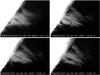 |
Fig. 1 Prominence of April 26, 2007 observed in the Hα line. Upper left: observations with the MSDP spectrograph of the Meudon Solar Tower. Upper right and lower: Hinode/SOT observations with the NFI. The field-of-view for all images is about 130″ × 100″. |
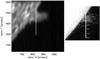 |
Fig. 2 Left: raster observations of SoHO/CDS (Coronal Diagnostic Spectrometer) (Harrison et al. 1995) in the Hei 584.33 Å line made on April 26, 2007 between 13:03:34 and 13:30:08 UT. The position of the SoHO/SUMER slit is marked. Right: Meudon/MSDP image of the prominence obtained in the Hα line centre at 12:47 UT overlaid with the contours of the same prominence observed from 13:03 UT with SoHO/CDS in Hei 584.3 Å line (image in the left panel). The position of SoHO/SUMER slit with respect to the Hα prominence is also marked. The numbers along the slit show the coordinates of the axis used in our work and the next figures. The length of the slit was 120″. Both images are plotted in the same spatial scale. For the analysis of the observed and theoretical prominence emission we used only the part of SoHO/SUMER spectra between 10″ and 46″. |
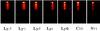 |
Fig. 3 Examples of the spectra of Lyβ, Lyγ, Lyδ, Lyε, Ly6, Ciii 977.03 Å, and Svi 933.40 Å lines observed by SoHO/SUMER spectrograph shortly after 13:00 UT, close to the time of the Meudon/MSDP observations. These spectra come from the whole SoHO/SUMER slit, i.e. the vertical size covers 120″. The wavelength width of all used spectra is between 3 and 4 Å. |
In the present paper we begin with a comparison of the integrated line intensities with previous 1D models. For that we use an extended grid of isothermal-isobaric models constructed by Gouttebroze et al. (1993) and further analysed by Heinzel et al. (1994). This follows the work done by Heinzel et al. (2001). But the main objective is to find an appropriate 2D RMHS model that explains current observations and takes into account the constraints provided by the Hα emission. The question is whether the non-reversed Lyman profiles are formed along the long axis of the magnetic dips (along the field lines) as we normally expect or if some other explanation is possible. The resulting model should provide us with the 2D structure of the magnetic dip filled with the prominence plasma. The critical parameter to be derived quantitatively is the plasma β. If we know this and can determine the magnetic-field orientation, we will be able to address various questions concerning the fine-structure dynamics as we see it from Hinode/SOT movies. Finally, we briefly address the question of hot bubbles (Berger et al. 2010), because we have data on selected PCTR lines.
The paper is organised as follows. In Sect. 2 we describe in detail our coordinated observations of the April 26, 2007 prominence. Section 3 presents the integrated line intensities. Description of 1D and 2D NLTE and RMHS models, together with results of modelling and line fitting, is the subject of Sect. 4. Finally, in Sect. 5 we summarize our results and discuss them in a broader context of high-resolution Hinode observations.
2. Observations of the prominence on April 26, 2007
The observations that we use in our work were obtained during a coordinated campaign of prominence studies. The campaign was performed between April 23 and 29, 2007 and many space instruments were involved: SOT, XRT, and EIS on Hinode, MDI, EIT, SUMER, and CDS on SoHO, TRACE, and several ground-based observatories: the Meudon Solar Tower (France), the Ondřejov Multicamera Spectrograph (Czech Republic), the MSDP Spectrograph in Wrocław (Poland) and others. This was the first Hinode-SUMER observing campaign dedicated to the study of prominences and filaments, investigating various aspects of their radiation, three-dimensional structure and the magnetic field.
On April 24, 2007, a long extended filament started to cross the limb (Török et al. 2009). On April 25, 2007, a part of the filament was clearly visible as a prominence and was intensively studied for its dynamics (Schmieder et al. 2010; Berger et al. 2010) and for its physical conditions by Heinzel et al. (2008). The next day, on April 26, 2007, another section of the filament crossed the limb. Hinode/SOT observations of this prominence exhibited many fine structures both in the Hα and Caii H line, which could be seen in the respective SOT movies. This prominence was also observed by Hinode/EIS (Labrosse et al. – submitted) and simultaneouly by MSDP of Meudon, SoHO/SUMER and by other instruments. Below we describe the observations used in our analysis.
2.1. Meudon/MSDP
The Multichannel Subtractive Double Pass (MSDP) (Mein 1991) spectrograph in Meudon is able to record two-dimensional maps of the Sun with the Hα-line profile in each pixel of the image. With the MSDP spectrograph operating on the Solar Tower of Meudon Observatory, the prominence was observed for three days of the campaign, on April 24, 25, and 26, 2007. On April 26 the prominence was observed between 12:19 and 12:54 UT, with a cadence of about 30 s. Sixty scans were collected during this time, some of them (about 10) are useless owing to the clouds passing the Sun. The times of the MSDP observations (images) used in this paper correspond to the beginning of the appropriate scan, each scan lasting about 20 s. The pixel size of the images is 0.4″, which gives fields-of-view of the images of 500″ × 465″. The spatial resolution depending on the actual seeing conditions is between 2″ and 3″.
After processing the data using the MSDP technique (Mein 1977, 1991) we obtained monochromatic images that allowed us to reconstruct the Hα-line profiles in all pixels of the image. The Hα-line profiles of the prominence were computed from 21 lambda-points and they can be extracted from the so called “p” files. Each “p” file contains 23 arrays: 21 for the profile, one for the sum and one for Dopplergram. The arrays used for the profiles are spaced by 0.1 Å, which means that the Hα-line profile can be used in the interval ± 1 Å from the line centre.
The MSDP observations of the prominence were calibrated photometrically using the Hα-line profile averaged over a quiet region on the disk in the vicinity of the prominence. The photometric calibration was done by fitting the mean observational quiet Sun profile to the standard atlas profile of the quiet Sun. In this analysis we used reference line profiles published by David (1961). In the processing we corrected the images for scattered light by analysing the signal of the MSDP images in the ambient corona. After these photometric corrections we obtained absolutely calibrated Hα-line profiles of the prominence.
In the obtained MSDP images we can see that the analysed prominence is of the quiescent type, with vertical threads and some arch-like structures (Fig. 1 – upper left panel). The prominence exhibited some brighter and darker structures and its shape is similar to that observed on April 25, 2007 (Schmieder et al. 2010).
2.2. Ondřejov/HSFA2
The Zeiss high-dispersion spectrograph working with the horizontal telescope – HSFA2 (Horizontal-Sonnen-Forschungs-Anlage 2) is designed for simultaneous spectroscopic observations of different solar features in several spectral lines (Kotrč 2009). It is installed at the Ondřejov observatory. On April 26, 2007, the HSFA2 spectrograph observed during the Meudon/MSDP and SoHO/SUMER observing times in several spectral lines, including Hα. From these observations we used the Hα spectra obtained at 13:19 UT to check our MSDP calibrations.
2.3. SoHO/SUMER
The prominence was observed by the SUMER (Solar Ultraviolet Measurements of Emitted Radiation) spectrograph (Wilhelm et al. 1995) on-board the SoHO (Solar and Heliospheric Observatory) satellite. Spectra in the wavelength range 900−1034 Å were observed. The prominence observations of April 26, 2007, were made in two long observational blocks − the first one was made between 05:55:08 and 07:57:30 UT and the second one between 13:01:34 and 23:50:04 UT. The position of the slit was static (the so-called sit-and-stare observations) and correction for the solar rotation was not switched on, which is a reasonable regime for off-limb observations. During the second observational block the slit was crossing the prominence, which is shown in Fig. 2. SoHO/SUMER was observing spectra in three spectral windows: 1025 Å, 972 Å and 939 Å. Observations in these spectral windows were made in the following sequence: 1025 Å, 972 Å, 939 Å, 939 Å, 972 Å, 1025 Å, etc. The exposure time of all observations was 115 s and they were made with a cadence of approximately 125 s. For all observations the detector B was used. The spectra of the wavelength range 989−1034 Å observed in the first spectral window (1025 Å) were obtained using the slit with dimensions of 0.99 arcsec × 120 arcsec. During the second observational block 79 observations in this spectral window were made. Profiles along the slit of the Lyβ line were taken from the spectra of the window. Spectra of the second spectral window (972 Å) of the wavelength range 934−979 Å were observed 79 times during the block using the slit with dimensions 0.99 arcsec × 120 arcsec. In the spectra, the following prominent lines were observed: Lyγ, Lyδ and Ciii 977.03 Å (on bare-part of the detector). The third spectral window (939 Å) was observed 80 times and spectra of wavelength range 900−945 Å were observed using the slit with dimensions 0.99 arcsec × 119.6 arcsec. The lines Sivi 933.40 Å, Lyε and higher Lyman-lines plus the Lyman continuum appear in the spectra of this spectral window.
The observed spectra were reduced and calibrated using standard SolarSoft procedures intended for the SoHO/SUMER data reduction. We reduced the data using the following procedures in this order: decompression of binary data saved in IDL-save files, dead-time correction, flat-fielding, local-gain correction, correction for geometrical distortion of the detector and finally the data were absolutely calibrated to erg/cm2/s/sr/Hz using the radiometry procedure (Schühle 2003, 2007). For a detailed technical information about the instrument, corrections and procedures see http://www.mps.mpg.de/projects/soho/sumer/text/webluca/ch_iust.html and references therein. For line identifications the SoHO/SUMER spectral catalogue (Curdt et al. 2001) was used. The spectrum image on the detector is inclined with respect to detector horizontal line because of a different orientation of the grating and the detector. This causes the spectra of the spectral lines with different wavelengths to be vertically shifted to higher or lower pixels on the detector. Moreover, there is an additional vertical shift owing to the displacement of the slit image on the detector caused by the nonlinearity of the grating focus mechanism (Schühle 2003). Vertical shifts caused by both effects together were computed for all used lines with the SolarSoft procedure delta_pixeland spectra were corrected for mutual shifts. The example of calibrated spectra of the lines Lyβ, Lyδ, Lyγ, Ciii 977.03 Å, Svi 933.40 Å and Lyε corrected for mutual shifts as observed by SoHO/SUMER at times close to the MSDP observations is shown in Fig. 3.
For the analysis of the line intensities of the prominence and for the construction of correlation plots we skip the part of the slit that cuts the solar disk, the edges of the prominence, and the long part crossing the dark sky. Therefore, we analysed the intensities between 10″ and 46″ counted along the slit from the north edge of the slit.
One of the crucial points for this analysis was a good photometric calibration of the Meudon/MSDP, SoHO/SUMER and Ondřejov/HSFA2 spectral observations. For the ground-based data we had to take into account not only the instrumental effects, but also an influence of the seeing. We estimated the uncertainty of all line intensities to be about 20%, including IINT. Another important parameter that may affect the results was the insufficiently accurate co-alignment of the observations obtained with different spectroscopic techniques and in different spectral ranges. Finally, we estimated the co-alignment uncertainty to be about 2−3″, which is comparable to the spatial resolution of the Meudon/MSDP, SoHO/SUMER and Ondřejov/HSFA2 data. Therefore, the co-alignment is not a critical problem in this analysis.
2.4. HINODE/SOT
The Hinode mission has been operating since October 2006 (Kosugi et al. 2007). The prominence studied here was well observed by the Hinode/SOT instrument on 25 and 26 April, 2007. The 50 cm diameter SOT can obtain a continuous, seeing-free series of diffraction-limited images in the 388−668 nm wavelength range with 0.2−0.3″ spatial resolution. In our study we use only Hα from SOT and we do not apply an unsharp mask procedure to increase the fine structure contrast (Schmieder et al. 2010). Looking at the Hα SOT movies from April 25, 2007, we see the evolution of the fine structures, particularly at the bottom of the prominence. The dynamics of this prominence was described in detail by Berger et al. (2010). Figure 1 presents some Hinode/SOT images of the prominence from April 26, 2007, where one can see a slow evolution of the prominence fine structures. The Hinode/SOT instrument starts the observations just after the Meudon/MSDP observations were finished because of clouds. Therefore, the time difference between the last MSDP image and first SOT image is 18 min.
2.5. Co-alignment of the observations
The crucial point of our work was the precise spatial co-alignment of all used observations of the prominence. We co-aligned the Meudon/MSDP, SoHO/SUMER and Hinode/SOT data. Although the closest time difference between Meudon/MSDP and Hinode/SOT was 17 min and the ground-based MSDP observations have no headers containing the pointing information, it was relatively easy to co-align these two sets of data. We simply found the positions of the images by maximizing the cross-correlation between images. The images showed in Fig. 1 are then co-aligned. It was much more difficult to co-align the Meudon/MSDP and SoHO/SUMER data. We do not have e.g. slit-jaw images for the SoHO/SUMER spectra that may be compared with MSDP. Therefore, we used the informations on the position of the slit contained in the SoHO/SUMER data and put the slit on the SoHO/CDS image raster observations in the Hei 584.33 Å line obtained between 13:03:34 and 13:30:08 UT (Fig. 2 – left panel). In this way we obtained some prominence image with the approximate position of the SoHO/SUMER slit. Next, we tried to co-align the MSDP Hα and SoHO/CDS Hei images to get the position of the SoHO/SUMER slit with respect to the prominence observed with MSDP. The co-alignment between MSDP and SoHO/CDS was not very precise because of the different appearance of the prominence in both images, which were taken at a different wavelength. The Hα emission of the prominence comes from the cool plasma and the UV Hei emission comes from other structures. Therefore, the size and morphology of the prominence differs in the two spectral lines and our co-alignment may be not very precise. Nevertheless, we estimated the precision of the position of the slit against the Hα prominence to be about 2″ (Fig. 2 – right panel).
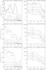 |
Fig. 4 Comparison of the calibrated integrated intensities of spectral lines emitted by the prominence. These intensities are plotted along the SoHO/SUMER slit for the part crossing the prominence (10−60″). The X-axis shows the position in arcsec along the SoHO/SUMER slit. We present the plots in linear scale to see the ratios of the intensities (left column) correctly and in logarithmic scale to better see the correlations between the curves (right column). Lyβ, Lyγ, Lyδ, Lyϵ, Ciii, and Sivi are obtained from SoHO/SUMER data. The Hα line was observed with Meudon/MSDP at 12:47 UT and is plotted with the SoHO/SUMER data only form 13:04 UT. The three raws correspond to different times of the SoHO/SUMER observations. For the Hα and Ciii lines (in linear plots) we used a scaling factor to properly place the curves within the graph. |
 |
Fig. 5 Correlation plots between the integrated intensities of the Hα, Lyβ and Lyγ lines. The stars represent Hα Meudon/MSDP and SoHO/SUMER observational points between 10″ and 46″ along the SoHO/SUMER slit (see Fig. 2). Other symbols correspond to the theoretical one-dimensional (1D) models at different temperatures (Gouttebroze et al. 1993): +: T = 6000 K, × : T = 8000 K, ◇: T = 10 000 K, △ : T = 15 000 K. |
3. Integrated intensities of the hydrogen lines
From the observed line profiles we calculated the integrated intensities of the analysed hydrogen lines to compare them with the results of theoretical NLTE calculations obtained for the GHV 1D models (Gouttebroze et al. 1993) and for the new 2D models of the prominence. Integrated intensities for a particular line represent the total energy radiated in this line and it may be easily compared with the theoretical values from the modelling. We were able to calculate the integrated intensities for the Lyman-hydrogen lines along the SoHO/SUMER slit in 120 points spaced by 1″. SoHO/SUMER slit was orientated in north-south direction. For the Hα line we calculated the integrated intensities also for 120 points along the 120″ line co-aligned with SoHO/SUMER slit. Therefore, each point along the SoHO/SUMER slit corresponds to the point along the line in Meudon/MSDP image.
Integrated intensities were calculated with the standard procedure, i.e. by integrating the specific intensities of the line profiles along the wavelength scale. The integration interval was ±1.2 Å for the Hα line from MSDP, and a few Å for the Lyman lines from SoHO/SUMER. From the SUMER data we also calculated the integrated intensities for the Ciii 977.03 Å and the Svi 933.40 Å lines. Figure 4 presents the observed calibrated integrated intensities along the whole 120″ SoHO/SUMER slit for three times of observations: 13:04, 13:16 and 13:47 UT. These times correspond to the mean time of the SoHO/SUMER observations. We present two kinds of plots – with the linear scale of the intensity axis (left column), and with the logarithmic scale of the intensity axis (right column). The reader may keep in mind that integrated intensities of the Hα line come from Meudon/MSDP observations at 12:47 UT, and they are plotted only in 13:04 UT plot (upper row). The time difference between the last Meudon/MSDP observations and the first SoHO/SUMER spectra is more than 17 min. Nevertheless, using the Hinode/SOT images (Fig. 1), we can assume that the evolution of the prominence was very slow, and in the Meudon/MSDP and the SoHO/SUMER data we practically analyse very similar large-scale structures. In addition, the Hα-line integrated intensity obtained at 13:19 UT from the Ondřejov/HSFA2 data is very similar to the integrated intensity obtained at 12:47 UT with Meudon/MSDP at the same position, which supports the assumption of a slow evolution of the prominence in the considered time.
It is interesting that the appearance of these integrated intensities differs significantly depending on the linear or logarithmic scale of intensity. With the linear scale the changes of the integrated intensities are better visible and we easily see the ratios of the different intensity curves. The logarithmic scale allows us to display all curves with a similar visibility, even though their intensities differ significantly.
The plots in the upper row of Fig. 4 correspond to the prominence observed at 13:04 UT in the Lyman and other UV lines (SoHO/SUMER) and to the prominence observed at 12:47 UT in the Hα line (Meudon/MSDP). The corresponding Hα image is presented in Fig. 2 – left panel. In the position around 15″ (X-axis) we can see a small depression of the Hα emission, which corresponds to the dark “bubble” structure visible close to the limb in the northern part of the prominence (Fig. 1 – upper left). A similar decrease of the integrated intensity is visible in the hydrogen Lyman, Ciii, and Sivi lines. Another depression is visible in the integrated intensities of all lines around 35″. Generally, in most parts of the curves we see good spatial correlations between the intensities of the Hα, Lyman, Ciii, and Svi lines. A similar situation is observed at other times (13:16 UT and 13:47 UT – middle and lower row of Fig. 4), where the spatial correlations between the intensity of all analysed lines is also high. For these times there are no corresponding Hα observations.
We also compared the integrated intensity of the Hα line observed with Ondřejov/HSFA2 spectrograph at 13:19 UT. It is a classical slit spectrograph, and therefore we were able to analyse only the emission of the prominence crossed by the slit of the spectrograph. The spatial orientation of the slit was not north-south as in SoHO/SUMER, but was inclined with respect to the SoHO/SUMER slit, and there is only one common crossing point of both slits. In this way we can use only one Hα-line profile from the area of the prominence observed simultaneously with SoHO/SUMER and Ondřejov/HSFA2. This point corresponds to the position of about 28″ along SoHO/SUMER and Meudon/MSDP slit and the Hα-line integrated intensity is 1.1 × 10⁵ erg cm-2 s-1 sr-1. This value is similar to the value obtained in the same position from the Meudon/MSDP data (1.2 × 10⁵ erg cm-2 s-1 sr-1). The small difference between these two values obtained from the two different ground-based instruments confirms the correctness of the photometric calibration of the data.
4. Observed and theoretical emission of the prominence
The integrated intensities obtained from the Meudon/MSDP and SoHO/SUMER observations were used for a comparison with the results of the theoretical NLTE modelling. We were able to use results from the 1D and 2D NLTE models.
4.1. 1D prominence slab models
Gouttebroze et al. (1993) have computed a set of 140 prominence NLTE models (GHV models) and Heinzel et al. (1994) made correlations of various plasma and radiation quantities. The models are represented by 1D vertical isobaric and isothermal slabs irradiated by the photospheric and chromospheric radiation. There are a few parameters that describe these models: gas pressure, temperature, geometrical thickness of the slab, microturbulent velocity and the height above the photosphere. A detailed description of the model grid is provided in Heinzel et al. (1994). The ranges of the variation of temperature, gas pressure, and geometrical thickness were 4300−15 000 K, 0.01−1.0 dyn cm-3, 200−10 000 km respectively.
From the synthetic line profiles obtained from GHV models it is possible to calculate the line integrated intensities (IINT). Heinzel et al. (2001) (Fig. 9) give IINT for the GHV models and presented theoretical correlation plots between IINT of different lines. For all analysed spectral lines the integrated intensities exhibited good mutual correlations for the Hα and for the Lyman lines. From the spectroscopic observations the authors also obtained few values of the integrated intensities for these lines and integrated them into the theoretical plots. The observational points fit the theoretical results for higher temperatures of the prominence models.
In our work we used 37 points along SoHO/SUMER slit and co-aligned Hα Meudon/MSDP data where we calculated IINT of lines. We integrated these values into the plots of Heinzel et al. (2001) to compare them with the theoretical emission from the 1D slab model. Figure 5 presents the correlation plots Hα – Lyβ, Hα – Lyγ, and Lyβ – Lyγ for the integrated intensities. We present theoretical points from the GHV models and the observational points (stars). The observational integrated intensities have a tendency to concentrate closer to the theoretical points that come from models with higher temperatures, 10 000 K for the Hα – Lyman lines plots, 15 000 K for the Lyman lines correlation plots. The gas pressure of the 1D models, which fits the observations, is between 0.05 and 0.2 dyn cm-2, depending on the geometrical thickness of the 1D model slab.
4.2. Modelling of 2D prominence fine structure
In this study we used the same 2D multi-thread modelling technique as in Gunár et al. (2008) and recently in Gunár et al. (2010). The model topology consists of a set of identical 2D fine-structure threads, which were first described by Heinzel & Anzer (2001) and subsequently analysed by Heinzel et al. (2005). The individual 2D threads are vertically infinite, and the variation of all physical quantities within them occurs in a horizontal plane parallel to the solar surface. They are in the magneto-hydrostatic (MHS) equilibrium with a prescribed (empirical) temperature profile. The 2D temperature structure is characterized by two different shapes of the PCTR. Within a narrow PCTR layer across the magnetic field lines (across B) the temperature exhibits a steep gradient between the central coolest part of the thread and its boundaries. In contrast to this, the temperature increases more gradually along the field lines (along B) within a fairly extended PCTR layer. This behaviour is caused by the large difference between the heat conduction along and across the magnetic field. These two PCTRs produce qualitatively different Lyman-line profiles (perhaps except for the strongest Lα line). In our previous work we have demonstrated that looking along B we mostly see non-reversed profiles, while looking across B the profiles are reversed. This provides certain diagnostics of the orientation of the magnetic field within the prominence body.
The multi-thread prominence topology that we used also in this study consists of Nidentical 2D threads, which are not subject to any mutual radiative interaction. When looking across the magnetic field, all individual threads are arranged perpendicularly to the LOS, with their long axis aligned along individual field lines (see Fig. 2 of Gunár et al. 2008). To simulate a random distribution of threads along this LOS, each thread is randomly shifted with respect to the foremost one. The LOS perpendicular to the magnetic field lines therefore intersects the individual threads at different positions along the long axis of each 2D thread. This then produces different emergent line profiles, integrated optical thicknesses, etc. We also used stochastically assigned LOS velocities for each thread, in the same way as Gunár et al. (2008, 2010).
On the other hand, when the LOS is aligned along the magnetic field lines, we see only one such thread because one field line cannot be dipped more than once.
In summary, we constructed 2D single thread models, but depending on the orientation of the LOS with respect to the magnetic field lines, we can see only this particular thread (along B) or several such threads (across B). To construct individual thread models, we have to solve a set of non-linear radiation-magneto-hydrostatic (RMHS) equations as described in Heinzel & Anzer (2001). This was done for a 5-level hydrogen model atom. Once the thread model is constructed for required input parameters, we solved NLTE problem in 2D for a 12-level hydrogen atom model to obtain the excitation and ionization equilibrium needed for the study of higher Lyman-lines. The final step was a formal solution of the transfer equation along the selected LOS (usually along or perpendicular to B) and this yielded the synthetic spectra that we compared with the observations.
4.3. Synthetic hydrogen spectra
We applied the modelling technique described above to obtain the synthetic spectra that would agree with a unique set of observed Lyman lines, obtained nearly simultaneously with the Hα line from the Meudon/MSDP (see previous sections). All syntetic hydrogen line profiles were convolved with a Gaussian function corresponding to the instrumental profile of Meudon/MSDP and SoHO/SUMER instruments.
The profiles of all observed Lyman lines exhibit only a non-reversed shape, which normally implies that the orientation of the magnetic field within the observed prominence should be parallel to the actual LOS (see e.g. Heinzel et al. 2001, 2005; Schmieder et al. 2007).
Therefore, by trial-and-error, we found an appropriate 2D model of a single thread that agrees well with the synthetic Lyman spectra obtained with the LOS orientated parallel to the magnetic field and the observed spectra. However, the corresponding synthetic Hα line exhibits a significantly lower intensity than the observed one and we were unable to find any other thread model that lead to a better agreement. However, we realized that the above model leads to similar, non-reversed Lyman-line profiles also for the LOS orientated perpendicularly to the magnetic field. This apparently contradicts our previous findings and thus deserves special attention.
A multi-thread structure viewed through B does not significantly affect the Lyman lines that are synthesized along the LOS perpendicular to the magnetic field (owing to the fairly high optical thickness of these lines and an absence of sharp peaks in their non-reversed profiles). But the synthetic Hα intensity significantly increases with the number of threads, because the optical thickness of this line is low, about unity. Then already for 20 threads the Hα line reasonably agrees with the observations, as will be discussed below. Note that the synthetic Lα-line profile is reversed as expected.
The input parameters of the present model are: the central (minimum) temperature T0 = 8000 K, the boundary PCTR temperature Ttr = 105 K, the maximum column mass in the centre of the thread (along the filed lines) M0 = 1.0 × 10⁻⁵ g cm-2, the horizontal field strength in the middle of the thread Bx(0) = 5 Gauss. The central and boundary pressures are pcen = 0.035 dyn cm-2 and ptr = 0.03 dyn cm-2, respectively. The central electron density is ne = 1010 cm-3. γ1 = 5 and γ2 = 30 are the exponents describing the gradients of the temperature within the PCTR, with γ1 representing the gradual rise of the temperature along the field lines from the thread centre towards its boundaries and γ2 prescribing the very steep temperature gradient across the field lines. The width of the thread across B (1000 km) is chosen arbitrarily, and the length of the thread along B (approximately 7500 km) is determined by the MHS equilibrium. Under these conditions, the column mass in the centre of the thread, across B, amounts to about 3 × 10⁻⁶ g cm-2 and the plasma β is 3.5 × 10⁻². We will refer to this model, which corresponds to the prominence of April 26, 2007, as Model2. It was derived by the trial-and-error method, and thus a minor change of the input parameters values (of the order of several percent) could lead to a slightly better agreement with the observed profiles. However, a 10% difference in the value of T0 and Bx(0) or a factor of two difference in some of the other input parameters leads to a model (such as Model1) with considerably different synthetic spectra from Model2 and thus to a worse agreement with the observations. Model1 was constructed by Gunár et al. (2007, 2008, 2010) to agree with the prominence observed on May 25 and 26, 2005, and we will discuss it in connection with our present analysis. To facilitate the comparison of Model1 and Model2 in Table 1 we show the input parameters for both models.
List of input parameters of Model1 and Model2.
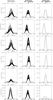 |
Fig. 6 Comparison between the observed Lyman lines and the Hα line, and the synthetic Lyman lines and the Hα line of the Model2. The left column displays the observed line profiles. The middle column shows the synthetic line profiles of the multi-thread Model2 with 40 threads obtained with the LOS perpendicular to the magnetic field. We display profiles emerging from 83 positions along the foremost thread of the multi-thread model. The right column displays the synthetic line profiles of the single-thread Model2 obtained with the LOS parallel to the magnetic field. We show the profiles in the middle of the thread (solid lines) and at one quarter distance from the thread boundary (dashed lines). |
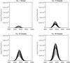 |
Fig. 7 Synthetic Hα-line profiles of Model2 obtained with the LOS perpendicular to the magnetic field for a single-thread model and for multi-thread models with 10, 20, and 40 threads. We display profiles emerging from 83 positions along the foremost thread of the multi-thread model. |
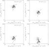 |
Fig. 8 Correlation plots between the integrated intensities of the Hα and Lyβ, Lyγ, Lyδ and Lyϵ lines. The stars represent the Hα Meudon/MSDP and SoHO/SUMER observational points between 10″ and 46″ along the SoHO/SUMER slit (12:47 UT for MSDP and 13:04 UT for SoHO/SUMER). Dots correspond to the theoretical two-dimensional model. In each panel there are 8300 theoretical points, 83 different line-of-sights for 100 different stochastic realizations for 40-threads system. |
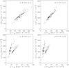 |
Fig. 9 Correlation plots between the integrated intensities of the hydrogen Lyman lines. The stars represent SoHO/SUMER observational points. Dots correspond to the theoretical two-dimensional model. In each panel there are 8300 theoretical points, 83 different line-of-sights for 100 different stochastic realizations for 40-threads system. For these plots we used a linear scale on both axes. |
Figure 6 shows the comparison between the observed Lyman lines and Hα, and the synthetic Lyman lines and the Hα line for Model2. The left column displays the observed Lyβ to Ly6 lines obtained by SoHO/SUMER and the Hα line obtained by Meudon/MSDP. We display 35 profiles for each Lyman line and 27 Hα-line profiles aligned with the SoHO/SUMER slit. In the middle column we show the synthetic Lyman lines and the Hα line for Model2 obtained with the LOS perpendicular to the magnetic field. We selected one particular randomly generated configuration of the 2D multi-thread structure with 40 threads and display the profiles emerging from 83 positions (the distance between individual positions is less than 100 km) along the foremost thread. The right column displays the synthetic profiles for Model2 obtained with the LOS parallel to the magnetic field. We show the profiles in the middle of the thread and at the one quarter distance from the thread boundary (because our threads are 1000 km thick, these positions represent 250 and 500 km from the thread boundary). Figure 6 clearly shows that the agreement with observations can be achieved only when the LOS is crossing the field lines. Hα plays a decisive role in this case. The comparison of the synthetic and observed profiles was performed only visually. Figure 7 shows the synthetic Hα-line profiles from Model2 obtained with the LOS perpendicular to the magnetic field, for a single-thread model and for multi-thread models with 10, 20, and 40 threads. We again display profiles emerging from 83 positions (the distance between individual positions is less than 100 km) along the foremost thread.
Integrated line intensities calculated from our model were also compared with the observations. We constructed plots where the correlations between the integrated intensities of different lines are presented (Figs. 8, 9). For the Hα and Lyman lines we can see that the concentration of theoretical points is very close to the observations, except for the plot Hα – Lyϵ, where the observed integrated intensities of Lyϵ are lower than the theoretical by about 50% (Fig. 8 – lower right). For the Lyman lines alone, the theoretical integrated intensities of Lyβ, Lyγ and Lyδ lines fit the observational correlations quite well (Fig. 9 – upper panels). However, for Lyϵ and Ly6 (Fig. 9 – lower panels) we again see that the observed integrated intensities are lower than the theoretical ones by some 50%. Preliminary tests with our 12-level model atom show that this can be caused by certain approximations in our treatment of the incident radiation in the subordinate line transitions.
5. Summary and discussion
We have presented a comparison between the observations of a quiescent prominence on April 26, 2007 in the hydrogen Lyman lines (Lyβ to Ly6) and Hα with the theoretical models obtained in 1D and 2D geometrical configurations. For the comparison we used the integrated intensities IINT obtained from spectroscopic observations of the prominence and from the synthetic line profiles of 1D and 2D models. As an additional constraint we used the profiles of all observed lines and made a statistical comparison of the line profiles with the results of multi-thread 2D modelling.
The integrated line intensities were always used to characterize the emission of a prominence in various spectral lines and to test the NLTE models (e.g. Heinzel et al. 2001). In the present analysis we were able to determine IINT in many different points of the prominence of April 26, 2007. The new feature is a quasi co-temporal detection of several Lyman lines above Lα together with Hα. All observed integrated intensities were plotted along the SoHO/SUMER slit (Fig. 4) and exhibit good spatial correlations in most cases. Note two different representations of the plots, on linear and log scales. From the linear plots we directly see the line ratios, while the log plots enhance the weaker lines. The emission in the Ciii and Svi lines could represent the emission of the PCTR of the prominence, while the hydrogen lines emission comes mainly from the cool core of the prominence. Nevertheless, we also observe a good spatial correlation between the emission in these “hot” and “cool” lines, even though the line formation temperatures are significantly different. This may give us some ideas about the nature of the “bubbles” recently discussed e.g. by Berger et al. (2010). Our analysis does not support the scenario that there is an excess of a hot plasma in the parts where the density of the cool plasma that emitts the hydrogen lines is low and this may drive an upflow of the bubbles. This conclusion is valid at least for the plasma of temperatures comparable to the formation temperature of the Ciii and Svi lines, i.e. respectively around 80 000 K and 200 000 K. Bubbles could be more magnetized, but it is impossible to measure the magnetic field in structures that have a very low signal in the cool lines used for the measurements. This topic of the bubbles and the mass flow in prominences is still open. A quantitative study of the prominence emission, especially in hotter lines, is necessary.
In this paper we constructed and analysed the correlation plots for the observed and theoretical values of IINT. First, we compared our observed IINT with the results of previous 1D models of the GHV (Gouttebroze et al. 1993; Heinzel et al. 1994). From the analysis of 37 data points we found that the observed integrated intensities have a tendency to concentrate close to theoretical points of the GHV models with higher temperatures, 10 000 K for the Hα – Lyman line plots, and 15 000 K for the Lyman line correlation plots (Fig. 5). These results are similar to those of Heinzel et al. (2001). However, a close inspection of the GHV line profiles that correspond to these models reveals their strong reversals. Because our observed Lyman-line profiles are unreversed, this clearly demonstrates a non-uniqueness of the model fitting when only the integrated line intensities are used.
As already pointed out by Heinzel et al. (2001), the problem is connected with the existence of a PCTR, which influences the emission in the Lyman lines and was not included in the GHV models. Therefore, our next step was fitting the Lyman profiles using the most sophisticated 2D multi-thread models. The Model1 of Gunár et al. (2007, 2008, 2010) gave reasonable integrated intensities, but all Lyman-line profiles were reversed. Our newly constructed Model2 of a single 2D thread leads to unreversed profiles with reasonable integrated intensities of all Lyman lines, when looking along or across B. However, we could no longer interpret the nonreversed profiles as being formed along B (like we did in our previous work), because the computed Hα intensity was much lower than the observed one (Fig. 6). Then, the only solution for keeping the Lyman lines almost unchanged and significantly enhance Hα was to look perpendicularly to B and add-up many threads. With 20−40 such 2D threads we finally achieved a very good solution.
Comparison of the theoretical hydrogen Lyman lines obtained with Model1 of a massive prominence (Gunár et al. 2010) with our new Model2 of a low mass prominence.
The model with 40 threads, which we used in the analysis, correctly reproduces all line intensities, including the Hα line. This is not surprising because other studies have also shown that 10−100 threads are required in prominence models (Mein & Mein 1991; Fontenla et al. 1996). However, the number of threads can be reduced if the LOS is inclined to the axis of threads. The number of threads mainly influences the intensity of the Hα line (Fig. 7), while the Lyman lines do not significantly change their intensity. This is because of the high optical thickness of the Lyman lines and low optical thickness of the Hα line. The theoretical relations between the integrated intensities of the analys ed lines correspond well to the observational relations in most cases. We can see a very good agreement between the position of observed and theoretical points in correlation plots (Figs. 8, 9). Only for the higher lines of the Lyman series is the agreement weaker.
Relations between the temperature of the prominence core, the presence of PCTR, the integrated line intensities and the Lyman-line profiles for Model1, Model2 and the GHV models.
Returning to the GHV, we can find models that have a quite similar cool core as our Model2 viewed through B. These are the models with T = 8000 K, p = 0.01−0.05 dyn cm-2 and a geometrical thickness of 1000 km, which lead to practically unreversed Lyman profiles. However, their integrated intensities are far too low compared to our observations. Compared to Model2, this again clearly indicates the importance of PCTR for Lyman-line emission in this prominence.
In Table 2 we summarize all considered situations and compare Model1 of Gunár et al. (2010) with our new Model2. Table 3 summarizes the behaviour of Model1 and Model2 when viewing the prominence along and across B, and compares them with the GHV models. This shows a critical importance of a PCTR for the intensity of the Lyman lines. The model with low pressure and PCTR can produce non-reversed line profiles even when the LOS ⊥ B. We can also see how the reversal of the Lyman lines above the Lα (which is almost always reversed, even when all higher lines are unreversed) depends on the temperature of the cool core, the central gas pressure, and the presence of a PCTR. Looking across B, two solutions are possible for a cool core with PCTR: high-pressure models with reversed profiles or low-pressure models with unreversed profiles. With a fixed geometrical thickness (1000 km in all our cases), this leads to lower or higher column mass across B.
Let us recall that the analysed prominence is a part of the same filament that crossed the limb on April 24 to 26, 2007. Other parts observed on April 25, 2007, have been extensively studied by several authors with different perspectives (Heinzel et al. 2008; Berger et al. 2010; Schmieder et al. 2010). The filament itself was very quiescent. It was observed during the solar minimum activity along a magnetic inversion line surrounded by weak magnetic polarities (maximum 10 Gauss in SoHO/MDI magnetograms). On the disk, a few days before, only the feet are detectable with bushes of threads. The main body between the feet is not visible. Low pressure (pcen = 0.035 dyn cm-2) and a low magnetic field (5 Gauss) in Model2 suggest that the prominence observed on April 26, 2007, is indeed a low-mass and weakly-magnetized structure. From our modelling the plasma β is 3.5 × 10⁻². Additional constraints on the model can be obtained with the Hinode/EIS spectra of the Heii 256 Å line (Labrosse et al. 2010 – submitted).
An important result of this study is that the whole set of observed lines in this particular prominence can be reasonably fitted only when the LOS intersects the magnetic field lines perpendicularly. The decisive role plays the Hα line. The plasma in individual threads is loaded within a dipped magnetic field, but in this case the dips are very shallow because of the low value of B in their centre (5 Gauss) and the relatively low-mass loading (low-pressure Model2). For the static case we explain quasi-vertical Hα threads by a pile-up of magnetic dips (see Heinzel & Anzer 2001; Dudík et al. 2008). Now, the obvious question arises: how can the small-scale Hα blobs seen in the Hα movie taken by Hinode/SOT give an impression of a constant downflow in a quasi-vertical direction in the plane of sky? This is a challenging problem, provided that these motions are not an artefact of the image processing. Fully dynamical models do not exist yet and thus we are limited to speculative scenarios. Perhaps we have to rule-out the propagation of a blob caused by a consecutive reconnection because the field lines are very shallow and cannot form a current sheet. But we may consider various projection effects within a fairly complicated 3D fine-structure topology. When we measured the transverse motion in the sky plane, the standard velocity was low and comparable to the Dopplershifts 1 to 5 km s-1 (Schmieder et al. 2010). These downflows are very difficult to measure even with the time-slice method. If there is any, it could be caused by a shrinkage of field lines. The motions would be also caused by the field itself, the plasma being moved with it – from our modelling the plasma beta is β is 3.5 × 10⁻². Another idea is that the plasma moves along the magnetic structures – in reality the dips have inclined field lines and thus the plasma can flow through their central part. The whole structure is certainly not static and can be shaken in the corona by different perturbations.
Acknowledgments
The work of A.B. was supported by the grant of the Academy of Sciences of the Czech Republic No. M100030942 and by the grant of the Czech Science Foundation No. P209/10/1680. S.G. acknowledges the support from grant 250/09/P554 of the Czech Science Foundation. This work was also supported by ESA-PECS project No. 98030 and the institutional project AV0Z10030501. The work of P.H. was supported by the grant of the Czech Science Foundation No. P209/10/1680 P.S. was supported by the grants of the Czech Science Foundation No. P209/10/1706 and P209/10/1680. Hinode is a Japanese mission developed and launched by ISAS/JAXA, with NAOJ as domestic partner and NASA and STFC (UK) as international partners. It is operated by these agencies in co-operation with ESA and NSC (Norway). We would like to acknowledge U. Anzer for many useful discussions and P. Kotrč and M. Zapiór for the data from Ondřejov/HSFA2 spectrograph. We thank our colleagues from the International Team 174 of the International Space Science Institute (ISSI) in Bern for their helpful discussions. The support of ISSI is gratefully acknowledged. This work was made in the frame of the SOLAIRE network supported by the European Commission (MTR-CT–2006-035484). The data presented here have been obtained during a coordinated campaign between Hinode, SoHO and GBOs (JOP 178, HOP111) organized by MEDOC in Orsay. The PI of the campaign was BS and the planners of SoHO/SUMER were S.G., and N. Labrosse. Thanks to them the prominence has been correctly pointed in the field of view of Hinode/SOT and SoHO/SUMER. A.B. and P.H. acknowledge the hospitality and support of the Paris Observatory.
References
- Berger, T. E., Slater, G., Hurlburt, N., et al. 2010, ApJ, 716, 1288 [NASA ADS] [CrossRef] [Google Scholar]
- Curdt, W., Brekke, P., Feldman, U., et al. 2001, A&A, 375, 591 [NASA ADS] [CrossRef] [EDP Sciences] [Google Scholar]
- David, K. 1961, ZAp, 53, 37 [Google Scholar]
- Dudík, J., Aulanier, G., Schmieder, B., Bommier, V., & Roudier, T. 2008, Sol. Phys., 248, 29 [NASA ADS] [CrossRef] [Google Scholar]
- Fontenla, J. M., Rovira, M., Vial, J., & Gouttebroze, P. 1996, ApJ, 466, 496 [Google Scholar]
- Gouttebroze, P., Heinzel, P., & Vial, J. C. 1993, A&AS, 99, 513 [NASA ADS] [Google Scholar]
- Gunár, S., Heinzel, P., Schmieder, B., Schwartz, P., & Anzer, U. 2007, A&A, 472, 929 [NASA ADS] [CrossRef] [EDP Sciences] [Google Scholar]
- Gunár, S., Heinzel, P., Anzer, U., & Schmieder, B. 2008, A&A, 490, 307 [NASA ADS] [CrossRef] [EDP Sciences] [Google Scholar]
- Gunár, S., Schwartz, P., Schmieder, B., Heinzel, P., & Anzer, U. 2010, A&A, 514, A43 [NASA ADS] [CrossRef] [EDP Sciences] [Google Scholar]
- Harrison, R. A., Sawyer, E. C., Carter, M. K., et al. 1995, Sol. Phys., 162, 233 [NASA ADS] [CrossRef] [Google Scholar]
- Heinzel, P., & Anzer, U. 2001, A&A, 375, 1082 [NASA ADS] [CrossRef] [EDP Sciences] [Google Scholar]
- Heinzel, P., Gouttebroze, P., & Vial, J. 1994, A&A, 292, 656 [NASA ADS] [Google Scholar]
- Heinzel, P., Schmieder, B., Vial, J.-C., & Kotrč, P. 2001, A&A, 370, 281 [NASA ADS] [CrossRef] [EDP Sciences] [Google Scholar]
- Heinzel, P., Anzer, U., & Gunár, S. 2005, A&A, 442, 331 [NASA ADS] [CrossRef] [EDP Sciences] [Google Scholar]
- Heinzel, P., Schmieder, B., Fárník, F., et al. 2008, ApJ, 686, 1383 [NASA ADS] [CrossRef] [Google Scholar]
- Kosugi, T., Matsuzaki, K., Sakao, T., et al. 2007, Sol. Phys., 243, 3 [NASA ADS] [CrossRef] [Google Scholar]
- Kotrč, P. 2009, Cent. Eur. Astrophys. Bull., 33, 327 [NASA ADS] [Google Scholar]
- Labrosse, N., Heinzel, P., Vial, J., et al. 2010, Space Sci. Rev., 151, 243 [Google Scholar]
- Mackay, D. H., Karpen, J. T., Ballester, J. L., Schmieder, B., & Aulanier, G. 2010, Space Sci. Rev., 151, 333 [NASA ADS] [CrossRef] [Google Scholar]
- Mein, P. 1977, Sol. Phys., 54, 45 [NASA ADS] [CrossRef] [Google Scholar]
- Mein, P. 1991, A&A, 248, 669 [NASA ADS] [Google Scholar]
- Mein, P., & Mein, N. 1991, Sol. Phys., 136, 317 [Google Scholar]
- Schmieder, B., Gunár, S., Heinzel, P., & Anzer, U. 2007, Sol. Phys., 241, 53 [NASA ADS] [CrossRef] [Google Scholar]
- Schmieder, B., Chandra, R., Berlicki, A., & Mein, P. 2010, A&A, 514, A68 [NASA ADS] [CrossRef] [EDP Sciences] [Google Scholar]
- Schühle, U. 2003, SUMER Data Cookbook, published on internet at http://www.mps.mpg.de/projects/soho/sumer/text/cookbook.html [Google Scholar]
- Schühle, U. 2007, personal communication [Google Scholar]
- Török, T., Aulanier, G., Schmieder, B., Reeves, K. K., & Golub, L. 2009, ApJ, 704, 485 [NASA ADS] [CrossRef] [Google Scholar]
- Wilhelm, K., Curdt, W., Marsch, E., et al. 1995, Sol. Phys., 162, 189 [NASA ADS] [CrossRef] [Google Scholar]
All Tables
Comparison of the theoretical hydrogen Lyman lines obtained with Model1 of a massive prominence (Gunár et al. 2010) with our new Model2 of a low mass prominence.
Relations between the temperature of the prominence core, the presence of PCTR, the integrated line intensities and the Lyman-line profiles for Model1, Model2 and the GHV models.
All Figures
|
Fig. 1 Prominence of April 26, 2007 observed in the Hα line. Upper left: observations with the MSDP spectrograph of the Meudon Solar Tower. Upper right and lower: Hinode/SOT observations with the NFI. The field-of-view for all images is about 130″ × 100″. |
| In the text | |
|
Fig. 2 Left: raster observations of SoHO/CDS (Coronal Diagnostic Spectrometer) (Harrison et al. 1995) in the Hei 584.33 Å line made on April 26, 2007 between 13:03:34 and 13:30:08 UT. The position of the SoHO/SUMER slit is marked. Right: Meudon/MSDP image of the prominence obtained in the Hα line centre at 12:47 UT overlaid with the contours of the same prominence observed from 13:03 UT with SoHO/CDS in Hei 584.3 Å line (image in the left panel). The position of SoHO/SUMER slit with respect to the Hα prominence is also marked. The numbers along the slit show the coordinates of the axis used in our work and the next figures. The length of the slit was 120″. Both images are plotted in the same spatial scale. For the analysis of the observed and theoretical prominence emission we used only the part of SoHO/SUMER spectra between 10″ and 46″. |
| In the text | |
|
Fig. 3 Examples of the spectra of Lyβ, Lyγ, Lyδ, Lyε, Ly6, Ciii 977.03 Å, and Svi 933.40 Å lines observed by SoHO/SUMER spectrograph shortly after 13:00 UT, close to the time of the Meudon/MSDP observations. These spectra come from the whole SoHO/SUMER slit, i.e. the vertical size covers 120″. The wavelength width of all used spectra is between 3 and 4 Å. |
| In the text | |
|
Fig. 4 Comparison of the calibrated integrated intensities of spectral lines emitted by the prominence. These intensities are plotted along the SoHO/SUMER slit for the part crossing the prominence (10−60″). The X-axis shows the position in arcsec along the SoHO/SUMER slit. We present the plots in linear scale to see the ratios of the intensities (left column) correctly and in logarithmic scale to better see the correlations between the curves (right column). Lyβ, Lyγ, Lyδ, Lyϵ, Ciii, and Sivi are obtained from SoHO/SUMER data. The Hα line was observed with Meudon/MSDP at 12:47 UT and is plotted with the SoHO/SUMER data only form 13:04 UT. The three raws correspond to different times of the SoHO/SUMER observations. For the Hα and Ciii lines (in linear plots) we used a scaling factor to properly place the curves within the graph. |
| In the text | |
|
Fig. 5 Correlation plots between the integrated intensities of the Hα, Lyβ and Lyγ lines. The stars represent Hα Meudon/MSDP and SoHO/SUMER observational points between 10″ and 46″ along the SoHO/SUMER slit (see Fig. 2). Other symbols correspond to the theoretical one-dimensional (1D) models at different temperatures (Gouttebroze et al. 1993): +: T = 6000 K, × : T = 8000 K, ◇: T = 10 000 K, △ : T = 15 000 K. |
| In the text | |
|
Fig. 6 Comparison between the observed Lyman lines and the Hα line, and the synthetic Lyman lines and the Hα line of the Model2. The left column displays the observed line profiles. The middle column shows the synthetic line profiles of the multi-thread Model2 with 40 threads obtained with the LOS perpendicular to the magnetic field. We display profiles emerging from 83 positions along the foremost thread of the multi-thread model. The right column displays the synthetic line profiles of the single-thread Model2 obtained with the LOS parallel to the magnetic field. We show the profiles in the middle of the thread (solid lines) and at one quarter distance from the thread boundary (dashed lines). |
| In the text | |
|
Fig. 7 Synthetic Hα-line profiles of Model2 obtained with the LOS perpendicular to the magnetic field for a single-thread model and for multi-thread models with 10, 20, and 40 threads. We display profiles emerging from 83 positions along the foremost thread of the multi-thread model. |
| In the text | |
|
Fig. 8 Correlation plots between the integrated intensities of the Hα and Lyβ, Lyγ, Lyδ and Lyϵ lines. The stars represent the Hα Meudon/MSDP and SoHO/SUMER observational points between 10″ and 46″ along the SoHO/SUMER slit (12:47 UT for MSDP and 13:04 UT for SoHO/SUMER). Dots correspond to the theoretical two-dimensional model. In each panel there are 8300 theoretical points, 83 different line-of-sights for 100 different stochastic realizations for 40-threads system. |
| In the text | |
|
Fig. 9 Correlation plots between the integrated intensities of the hydrogen Lyman lines. The stars represent SoHO/SUMER observational points. Dots correspond to the theoretical two-dimensional model. In each panel there are 8300 theoretical points, 83 different line-of-sights for 100 different stochastic realizations for 40-threads system. For these plots we used a linear scale on both axes. |
| In the text | |
Current usage metrics show cumulative count of Article Views (full-text article views including HTML views, PDF and ePub downloads, according to the available data) and Abstracts Views on Vision4Press platform.
Data correspond to usage on the plateform after 2015. The current usage metrics is available 48-96 hours after online publication and is updated daily on week days.
Initial download of the metrics may take a while.