| Issue |
A&A
Volume 530, June 2011
|
|
|---|---|---|
| Article Number | A8 | |
| Number of page(s) | 14 | |
| Section | Stellar structure and evolution | |
| DOI | https://doi.org/10.1051/0004-6361/201014319 | |
| Published online | 27 April 2011 | |
Oxygen- and carbon-rich variable red giant populations in the Magellanic Clouds from EROS, OGLE, MACHO, and 2MASS photometry
1
Nicolaus Copernicus Astronomical Centre, Bartycka 18,
00-716
Warsaw,
Poland
2
UPMC Université Paris 06, UMR 7095, Institut d’Astrophysique de
Paris, 75014
Paris,
France
e-mail: marquett@iap.fr; beaulieu@iap.fr; lesquoy@iap.fr
3
CNRS, UMR 7095, Institut d’Astrophysique de Paris,
75014
Paris,
France
4
Adam Mickiewicz University Observatory,
ul. Słoneczna 36,
60-286
Poznań,
Poland
e-mail: alex@camk.edu.pl
5
Research School of Astronomy & Astrophysics, Mount
Stromlo Observatory, Cotter
Road, Weston
ACT
2611,
Australia
e-mail: tisseran@mso.anu.edu.au
6
CEA, DSM,
DAPNIA, Centre d’Études de Saclay, 91191
Gif-sur-Yvette Cedex,
France
Received: 24 February 2010
Accepted: 8 March 2011
Context. The carbon-to-oxygen (C/O) ratio of asymptotic giant branch (AGB) stars constitutes an important index of evolutionary and environment/metallicity factor.
Aims. We develop a method for mass C/O classification of AGBs in photometric surveys without using periods.
Methods. For this purpose we rely on the slopes in the tracks of individual stars in the colour-magnitude diagram.
Results. We demonstrate that our method enables the separation of C-rich and O-rich AGB stars with little confusion. For the Magellanic Clouds we demonstrate that this method works for several photometric surveys and filter combinations. As we rely on no period identification, our results are relatively insensitive to the phase coverage, aliasing, and time-sampling problems that plague period analyses. For a subsample of our stars, we verify our C/O classification against published C/O catalogues. With our method we are able to produce C/O maps of the entire Magellanic Clouds.
Conclusions. Our purely photometric method for classification of C- and O-rich AGBs constitutes a method of choice for large, near-infrared photometric surveys. Because our method depends on the slope of colour-magnitude variation but not on magnitude zero point, it remains applicable to objects with unknown distances.
Key words: methods: data analysis / techniques: photometric / surveys / stars: oscillations / stars: AGB and post-AGB / Magellanic Clouds
© ESO, 2011
1. Introduction
Low and intermediate mass stars evolve through three late stages. After passing the red giant branch (RGB) they reach maximum luminosity at its tip (TRGB) followed by a luminosity drop after the helium flash. Next they grow again and move along the asymptotic giant branch (AGB). According to their spectra, the AGB stars split into oxygen-rich stars (O-rich, M-stars, or K-stars) and carbon-rich stars (C-rich, C-stars, or N-stars). The M-stars have more oxygen than carbon in their atmospheres (C/O < 1). When the abundance of oxygen equals that of carbon the AGB type is S. Classification of the latter is difficult and also involves intermediate MS and SC types (Cioni & Habing 2003).
Stars entering the AGB phase are rich in oxygen; however, subsequent dredge-up caused by thermal pulsation may enrich their atmospheres in carbon (Iben & Renzini 1983). On the AGB, several thermal pulses (TP-AGB) may occur, resulting in dredging up the matter enriched in carbon nuclei by nuclear fusion. In this way the O-rich stars are converted after at least several pulses into the C-rich ones (Marigo et al. 2008, and references there).
It is believed that the rate of conversion of O-stars into C-stars depends on the efficiency of the third dredge-up and the extent and time variation in the massloss (e.g. Iben 1981; Marigo et al. 1999). Mass loss is expected to be stronger in metal-rich stars, giving to shorter AGB life and eventually yielding a C-star. These thermal pulses result in the luminosity variations with the peak-to-peak amplitude up to a few magnitudes at visual wavelengths.
According to Iben & Renzini (1983), the lower the metallicity the less carbon needed to be dredged-up in order to convert an O-star into a C-star, hence the correlation between metallicity and the C/M ratio. For lower metallicity, the AGB evolutionary tracks move to higher temperatures; for very low metallicity a post-horizontal-branch star may become a white dwarf without first becoming an AGB star. Since O and C stars reveal very different spectra, it is relatively easy to spectroscopically identify C-rich stars even at large distances. The differences in molecular blanketing and dust creation result in an observed sharp dichotomy in infrared colours of O- and C-rich stars. Thus the O- and C-stars are often identified using narrow filters. The J − K colour of the C-rich stars is >1.4 mag and systematically redder than that of O-rich stars (Frogel et al. 1990; Costa & Frogel 1996; Cioni et al. 2000a). These effects influence the luminosity function of O- and C-rich AGB stars. The Magellanic Clouds are good test-beds of theories of the late stages of stellar evolution. They are nearby and yet far enough to ignore the LMC thickness, so that all stars are approximately at the same distance.
Late evolutionary stages are often associated with long period- (LPV), semi-, and irregular-variability. A wealth of data on this variability was collected as a by-product of the microlensing surveys. All yielded catalogues of numerous variable stars. In these data the period-luminosity relations of the LPV’s on the AGB are well documented for both the Large and Small Magellanic Clouds (Wood et al. 1999; Wood 2000; Cioni et al. 2001, 2003; Noda et al. 2002, 2004; Lebzelter & Hinkle 2002; Ita et al. 2004a,b; Kiss & Bedding 2003, 2004; Soszynski et al. 2004a,b, 2005; Groenewegen 2004; Fraser et al. 2005; Raimondo et al. 2005).
The period-luminosity diagram for red variables at advanced evolutionary stages reveals six sequences for different classes of objects (Ita et al. 2004b). Miras and some low-amplitude semiregulars pulsating in the fundamental mode form the sequence C. Other semiregular stars pulsating in the second and third overtone modes occupy sequences A, B, and C, and the RGB eclipsing binaries form their own sequence E. The origin of the sequence D corresponding to long-secondary periods (LSP) remains ambiguous. Wood et al. (2004) considered a number of possible explanations of LSP (radial and non-radial pulsations, rotations, orbiting companions, chromospheric activity, orbiting dust clouds), but none fit the observations satisfactorily.
Soszynski et al. (2004a) combined the OGLE-II and OGLE-III data and found the multiperiodicity of the red giants to be variable with a small amplitude. They exhibited two modes closely spaced in their power spectrum. This is likely to indicate non-radial oscillations. They also show that members of the short-period P–L sequences below the TRGB constitute a mixture of the RGB and AGB variables. Recently, Soszynski et al. (2004a, 2005); Soszyński (2007), and Derekas et al. (2006) have demonstrated that the sequence E overlapped with the sequence D, which may be evidence for a binary origin of the sequence D.
There are differences between the O-rich and C-rich LPVs, too. Cioni et al. (2003) note that C-stars have a larger amplitude than O-stars. Ita et al. (2004a) confirm that O- and C-rich Miras follow different period vs. (J − K) colour relations (Feast et al. 1989). The I-band amplitude of C-rich Miras tends to grow with the redder mean (J − K) colour, while the amplitude of O-rich Miras is colour independent (Matsunaga et al. 2005).
The evidence has provided new and significant constraints for theoretical pulsation models. Models and observations are compared in three ways: using stellar isochrones (e.g. Bressan et al. 1996; Bruzual & Charlot 2003; Mouhcine 2002; Marigo et al. 2003; Groenewegen & de Jong 1993), stellar tracks (Groenewegen & de Jong 1993; Marigo et al. 1999; Mouhcine & Lançon 2002; Lançon & Mouhcine 2002; Mouhcine & Lançon 2003), and the fuel consumption theorem by Renzini & Buzzoni (1986) and Maraston (1998, 2005).
The synthetic characteristics of AGB stars are derived either from complete evolution tracks, semi-empirical fits to the core mass-luminosity relation, or from the core mass-interpulse period relation and the mass-loss rate as a function of stellar parameters. The examples of such calculations are provided by Groenewegen & de Jong (1993) and Izzard et al. (2004).
Recent attempts have been made to include the TP-AGB phase in evolutionary population synthesis models. Both improvements in the low-temperature opacities and peculiarities of the actual surface chemical composition have such profound consequences that the whole AGB evolutionary scenario became significantly affected (Marigo et al. 2008). Use of the molecular opacities reflecting the actual chemical composition leads to a significant decrease in Teff as soon as C/O > 1 (Marigo et al. 2008, and references therein). This decrease is confirmed by observations of galactic AGB stars (Bergeat et al. 2001; Marigo et al. 2003), and it naturally explains the presence of a red tail in the (J − K) colour–magnitude diagram of C stars.
The mass loss is driven by pulsation in a complicated way. The pulsation pushes a fraction of the atmosphere above the photosphere, creating a cool and dense environment where dust grains form and grow efficiently. The radiation pressure on the dust combined with the momentum carried in the shock waves drives the mass loss (e.g., Wood 1979; Bowen & Willson 1991; Hoefner et al. 1996)
Lebzelter & Wood (2005) compared the observations of LPV in 47 Tuc with the models. On one hand, they find that the models without mass loss fail to reproduce the observed periods of the small amplitude pulsators. On the other, the K − log P sequence of the large amplitude variables, such as the Miras, is inconsistent with the mass-loss models and consistent with the no mass-loss models. Only models involving the non-linear fundamental mode yield periods consistent with the Miras in 47 Tuc (Olivier & Wood 2005).
The past decade has brought results of extensive photometric surveys – OGLE (Paczynski et al. 1994), OGLE II (Udalski et al. 1997), EROS (Aubourg et al. 1995), MACHO (Alcock et al. 1997), and MOA (Bond et al. 2001) – covering several optical and infrared bands, sometimes simultaneously. They have provided a wealth of observations of red variable stars, thus enabling the study of their population properties. In particular, use of infrared colours and/or pulsation periods have enabled the classification of C- and O-rich stars. We discussed above the relevant observational and theoretical results.
In the present paper, we attempt to analyze the photometric properties of red variables in the visual region without recourse to their periods. Our analysis should be complementary to any traditional methods while suffering less, if at all, from aliasing and seasonal interference. We employ correlation slopes of colour and magnitude variability introduced by Wood et al. (2004). In this paper the slope aR of the correlation of R magnitude and V − R colour variations revealed no relation with any other property of red variables. We employ a different filter combination in our attempt of photometric classification of C and O-rich red variable stars. Our results should not depend much on the number of pulsation cycles covered by a given survey. Our practical requirement that data span at least one pulsation cycle, is met in most large surveys.
In Sect. 2 we describe data employed in the present study. Our calculation methods are described in Sect. 3. In Sect. 4 we propose new methods of selection O- and C-rich stars. Due to large differences in filters and time span, we present our results for each survey separately. We give an estimate of the C/O ratio for variable stars in the Magellanic Clouds. In Sect. 5 we employ a simple model to demonstrate how observed effects may arise. Possible peculiar variables are discussed in Sect. 6. We conclude in Sect. 7.
2. The data
Our paper is based primarily on the EROS-2 photometric survey of the Magellanic Clouds cross-referenced with the 2MASS infrared magnitudes (Sect. 2.1). We explicitly indicate when these are supplemented by the OGLE and MACHO photometry and four catalogues of C-and O-rich stars (Sects. 2.2–2.4).
2.1. EROS-2 survey
The Expérience de Recherche d’Objets Sombres (EROS-2) project employed extensive photometry obtained with the 1-m MARLY telescope at La Silla Observatory, Chile, to search for the baryonic dark matter of the Galactic halo by means of the gravitational microlensing (Afonso et al. 2003; Lasserre et al. 2000; Palanque-Delabrouille et al. 1998; Tisserand et al. 2007). The observations were performed between July 1996 and February 2003 through a dichroic plate-splitting light into two wide field cameras covering 0.7 × 1.4° in right ascension and declination each, yielding two broad passbands. The so-called blue channel (420–720 nm, hereafter BE band) overlapped the standard V and R standard bands, while the red one (620–920 nm, hereafter RE band) roughly matched the standard I filter. Each camera constituted a mosaic of eight 2k × 2k CCDs with a pixel size on the sky of (0.6′′)2.
Ten fields covered the SMC and 88 fields covered the LMC. The photometry from individual images was combined into light curves using the Peida package developed specifically for the EROS experiment (Ansari 1996). The estimated accuracy of this photometry is discussed by Derue et al. (2002). For uniformity, the SMC data were analysed again with the more recent version of Peida.
The RGB and AGB variable stars were selected from the SMC and LMC lists of EROS variables using their location in the colour-magnitude diagram. In this way we selected 28 914 stars in LMC and 5930 in SMC. They constitute our sample used in further analysis.
2.2. OGLE data
The Optical Gravitational Lensing Experiment (OGLE-II) data were collected with the 1.3 m Warsaw Telescope at the Las Campanas Observatory, Chile, operated by the Carnegie Institution of Washington. The I-band data span about 3000 days: from January 1997 to April 2005. The V-band measurements were obtained from 1997 to 2001 (Zebrun et al. 2001), so they span a shorter time baseline. Up to 70 V-band points per star are available. In the I-band, 500 to 900 measurements were available, depending on the field (Soszynski et al. 2005). In the present work we use data on 3586 LPV from LMC published by Soszynski et al. (2005), downloaded from the OGLE homepage1.
We cross-identified EROS and OGLE objects within a 1.3′′ radius. The OGLE-II fields cover only the bar of LMC, i.e. a much smaller field than for EROS, hence there are relatively few stars in common.
2.3. MACHO data
The MAssive Compact Halo Objects (MACHO) project (Alcock et al. 1997) comprises eight years of observations of the Large and Small Magellanic Clouds and of the Galactic Bulge. For the present purposes we selected LMC stars from the MACHO catalogue of variable stars (Alcock et al. 2003). Using the MACHO2 interface, we downloaded 2868 individual light curves of the stars classified as the red giant variables (classified as Wood A, B, C, and D sequences).
2.4. 2MASS survey data
The Two Micron All Sky Survey (2MASS)3 employed two 1.3-m robotic telescopes, one at Mt. Hopkins, Arizona, and one at CTIO, Chile. Each telescope was equipped with a three-channel camera, capable of observing the sky simultaneously at J (1.25 microns), H (1.65 microns), and Ks (2.17 microns). The southern facility began collecting Survey data in March 1998 and conducted its final scan in February 2001.
We extracted 2MASS data for each of the EROS fields separately. Then cross-identification was done separately for each field. During the cross-identification of EROS and 2MASS, we employed a 3′′ search radius. We selected only stars with photometry available in all three bands J, H, and Ks. AGB stars are among the brightest stars of the LMC. If an area of the order of 16 square degrees contains 25 000 AGB stars, their average separation is 1.5 min of arc, so the probability of blending two of them within the search radius is (1.5 ∗ 60 /3)-2 = 0.0006, thus corresponding to fewer than 15 stars in the whole sample. This is negligible compared to the blur of our photometric plots. At this point it is worth discussing the contamination of our AGB sample of IR colours with mistaken cross-identification with RGB stars. For stars brighter than TRGB (K < 12 for LMC and K < 12.7 for SMC), this problem does not exist. Suppose, for an EROS AGB star, that IR colours for an RGB one were fitted, then the star would land leftwards of the vertical lines on aV versus K diagrams. One possible problem is mixing faint AGBs with RGBs, causing pollution of RGBs with AGBs but not otherwise [i.e. faint AGB remain clean, if possibly incomplete]. Kiss & Bedding (2004) consider the same problem in more detail for stars from OGLE and 2MASS and conclude that contamination is insignificant, possibly no more than 0.3%, for their search radius of 1′′, corresponding to less than 3% contamination for our radius of 3′′. Since there were selected MACHO objects than for EROS, we cross-identified MACHO and 2MASS without subdivision into fields and with the same 3′′ radius. Again we only selected stars with photometry in all three bands J, H, and Ks.
2.5. The catalogues of C-rich stars
We selected 1707 C-rich stars from the SMC identified by Rebeirot et al. (1993) in the low-resolution spectroscopic survey employing the ESO 3.6 m telescope and 1185 stars identified in the Siding Spring Observatory survey by Morgan & Hatzidimitriou (1995).
A catalogue of 7760 C-rich stars in the LMC was presented by Kontizas et al. (2001). These stars were identified during a systematic survey of the objective-prism plates taken with the UK 1.2 m Schmidt Telescope. To these we added the list of C-rich stars from Groenewegen (2004).
Soszynski et al. (2005) demonstrate a new method of distinguishing between O-rich and C-rich Miras, SRVs and stars with long secondary periods, relying on their V and I-band photometry and periods. The list of stars selected from the LMC in this way was downloaded from the OGLE homepage. All C-rich stars from these catalogues were cross-identified with the EROS and MACHO stars within a 3′′ radius.
3. Data pre-processing
The analysis outlined in this paper was performed separately for EROS LMC and SMC, OGLE LMC and MACHO LMC data. We used data from all surveys to study a path in the colour–magnitude diagram traversed by each variable star. We investigated correlation of the average slope of the path with the chemical composition of the objects. The results of this analysis are summarised in diagrams described in Sect. 4.
The EROS survey produced simultaneous light curves in two spectral bands. By applying time filters to each band light curve we obtained a smooth, low-pass filtered light curve and its complementary high-pass light curve. The sum of the two reproduces the original light curve. In this way for each spectral band we obtained 3 light curves: raw, low-, and high-pass, six in total. In further analysis we study correlations of stellar properties with the properties derived from these light curves.
3.1. Photometric calibrations
Both EROS and MACHO obtained simultaneous expositions in two bands termed “red” (RE and r, respectively) and “blue” (VE and v, respectively) for nearly all observations. We simply ignored observations made in just one filter.
 |
Fig. 1 Sample EROS light curves for two stars with spectral types assigned by Cioni et al. (2001): DCMC J052618.12-694100.0 of type C (top row) and DCMC J052446.91-694949.9 of type M (bottom row). The left, middle, and right panels present the raw, low-pass, and high-pass light curves, respectively. For details of filtering see Sect. 3.2 |
Following Tisserand et al. (2007), we converted the raw photometry into the standard Kron-Cousins system using the following relations:  The MACHO data from the web database are available in the raw instrumental system. Following Alcock et al. (1997), we converted the raw photometry into the standard Kron-Cousins system using the following relations:
  where v and r are instrumental magnitudes and VMACHO and RMACHO are in the Kron-Cousins standard system. These calibration formulae are estimated to have an overall absolute accuracy of ± 0.10 mag in VMACHO or RMACHO and ± 0.04 mag in (V − R)MACHO (Alard et al. 2001).
The OGLE survey employs one camera, so observations in different filters are not simultaneous. Observations in V filter were obtained much less frequently than in I. For each V observation, we searched the nearest I observations. If two I points before and after a V observation separated by no more than 2 days, we performed a linear interpolation at the time of V observation. For just one I point nearby, no more than one day from the V observation, we assume they were measured nearly simultaneously. In this way for most V observations we found its corresponding I magnitudes. Other V observations were ignored. Because we only analyse stars with long periods, this procedure proved reliable for our purposes.
3.2. Time filtering
Through the whole paper except for Sect. 6, we used the raw light curves. Light curves for Sect. 6 were filtered in the time domain. The low-pass curve was obtained from the raw one by means of the “moving median”. The purpose of time filtering is to separate short period pulsations in some stars from the LSP. Since our procedure does not depend on actual detection of these periods, we applied it to all EROS red variables. We selected a window of width w centred on a given point and replaced its value with the window median value. In practice we filtered each light curve twice consecutively using windows of width w1 and w2 dependent on average Ks luminosity: 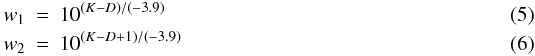 where the D magnitude is equal to 19.4 for the LMC and to 21.1 for the SMC. These windows were selected to have intermediate length between the short period and LSP (see Sect. 6 for discussion of these periods). As both periods depend on mean stellar brightness K, so do our window widths. The slope of − 3.9 corresponds to a border line between the short period sequences and the LSP sequence in the period-luminosity (P − L) diagram (Ita et al. 2004b; Soszynski et al. 2004a). As this area is virtually devoid of stars, its exact value is of no consequence for the current considerations.
We found that a light curve smoothed with two moving medians reveal LSP more clearly than when smoothed only once. Any short-period variations are filtered out. The high pass curve was obtained by subtracting the low pass one from the raw data. Only short time variations are left in the high-pass light curve. Sample light curves are plotted in Fig. 1. A similar procedure was employed by Wood et al. (2004) except that we did not use the short period as the parameter determining filter window to avoid confusion for multi-periodic/irregular red giants (Soszynski et al. 2004a). For EROS and MACHO colours (V − I)EROS, (V − R)MACHO were calculated for each time point. Subsequently we filtered colours similarly to how magnitudes are filtered. In this way we got the colour variation for raw data, LSP, and short time scale variations separately. For OGLE the number of V observations was too small to filter.
3.3. Analysis of colour variations
In further analyses we considered variations in colour against magnitude, for all possible combinations of light curves (raw, long-, and short-time scale colours against raw, long- and short-time scale V and I magnitudes). Sample plots are presented in Fig. 2. Next we fitted by the least squares the regression lines,  where aV and aI denote the slope of the corresponding colour–magnitude relation. This kind of linear equation was fitted for EROS, OGLE and MACHO data.
To verify the quality of our slope parameter, we calculated the correlation coefficient ρ and the statistic t in the following way: ![\begin{eqnarray} \label{e4.1} \rho &=& \frac{Cov\{V,V-I\}}{\sigma_{V}\sigma_{V-I}} \\ \label{e4.2} t &=& \frac{\rho}{\sqrt{1-\rho^2}}\sqrt{n-2} \mbox{~~~where}\\ \label{e4.0} Cov\{V,V-I\} &=& \frac{1}{n}\sum_{i}^{n}(V-\overline{V})\left[V-I-\overline{(V-I)}\right]. \end{eqnarray}](/articles/aa/full_html/2011/06/aa14319-10/aa14319-10-eq51.png) Results are shown in Fig. 3. For the null hypothesis H0 assuming no correlation, i.e. ρ = 0, a t statistic obeys the Student distribution with n − 2 degrees of freedom, where n is number of points per star (Fisz 1963). For a probability of 0.995, t is equal to 2.6. For most stars the correlation coefficient is greater than 0.5, and t is as significant as 15 or more.
Results are shown in Fig. 3. For the null hypothesis H0 assuming no correlation, i.e. ρ = 0, a t statistic obeys the Student distribution with n − 2 degrees of freedom, where n is number of points per star (Fisz 1963). For a probability of 0.995, t is equal to 2.6. For most stars the correlation coefficient is greater than 0.5, and t is as significant as 15 or more.
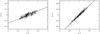 |
Fig. 2 Sample plot of raw colour and magnitude variations for the same 2 stars as in Fig. 1. We also plot the regression lines. Their inclination parameter is aV, discussed in the text. |
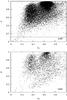 |
Fig. 3 Plot of the colour–magnitude correlation coefficient against the slope of magnitude-colour relation, for EROS LMC and SMC data. The correlation coefficient serves as a measure of quality of the slope av. The horizontal lines correspond to probability 0.995 of the null hypothesis H0, i.e. points lying above correspond to statistically significant correlation. |
3.4. Analysis of amplitude variations
The amplitude of the luminosity variation was calculated from the distance of the maximum and minimum in the corresponding, possibly filtered light curve. We derived the amplitude of the colour variation as the distance between points on these lines corresponding to extreme magnitudes. In this way we diminished the influence of individual colour errors on the colour amplitude. These amplitudes were calculated for each filter, and raw, long-, and short time-scale data.
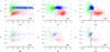 |
Fig. 4 Plots depicting three methods of distinguishing O- and C-rich variable stars (from left to right): slope-colour amplitude aV(ampVI), slope-K magnitude aV(K) and slope-J − K colour aV(J − K), for EROS LMC (top) and SMC (bottom) data. Vertical lines indicate adopted TRGB dividing RGB and AGB stars. See text for a detailed description of the methods and parameters of the boundaries. Black, dark grey, and light grey dots (blue, red, and green in electronic edition) respectively mark O- and C-rich AGB stars and O-rich RGB ones, classified using K magnitudes for AGB/RGB and leftmost panels for O/C content. |
4. Photometric chemical classification of red variable stars
4.1. The slope-amplitude diagram
Wood et al. (2004) have introduced the variability slope parameter aR. They note it has no obvious relation to any other property of red variable stars. Noticing that red giants have greater amplitude in the blue filter results in better accuracy for the slope estimates. We adopted the aV slope parameter as a better substitute. In the left panels of Fig. 4 we plot the slope aV of the colour–blue magnitude relation against amplitude, for all EROS red variable stars in the LMC and SMC. For completness we also plot aV against the near infrared magnitude and colour in the middle and right panels. In the rest of the present section, we investigate our slope parameter aV as a tool for the chemical and/or evolutionary status classification of red variable stars. We defer a discussion of the classification corresponding to the middle and right panels until Sects. 4.3 and 4.4. Anticipating our result, we adopted in Fig. 4 different colour coding for O-rich RGB stars, O-rich, and C-rich AGB stars as green(light grey), blue(black), and red(dark grey) dots, respectively. The colour-coded selection, for all diagrams, comes from the third method presented in the right panels.
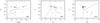 |
Fig. 6 Similar plots as in Fig. 4 for C-rich, O-rich, and intermediate stars of Cioni et al. (2001), of respective spectral types C (triangles), M (circles), and S (squares). |
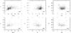 |
Fig. 7 C-rich stars in LMC (upper panels) from Kontizas et al. (2001) and Groenewegen (2004) and in SMC (lower panels) from Rebeirot et al. (1993) and Morgan & Hatzidimitriou (1995). Colour-slope parameter aV in function of: amplitude of colour change ampVI (left panels); K 2MASS magnitude (middle panels); J − K colour (right panels). |
The left panels in Fig. 4 display plots of the slope aV against the colour amplitude ampVI for EROS LMC and SMC data, respectively. Note the conspicious two-modal distribution of aV suggesting separate clustering of C- and O-rich AGB stars. In these plots there are two distinct branches corresponding to steep and shallow slopes, i.e. for large and small aV. For both branches, the slope initially grows and then, for amplitudes over 0.3, saturates at the constant values of 0.65 and 0.3. These two groups can be separated by the curve with the equation  (12)The same border holds for both EROS LMC and SMC data. In the following sections we demonstrate by cross-checking in the catalogues that the stars above and below the curve are respectively O- and C-rich. Thus our Eq. (12) constitutes the new classification criterion for C- and O-rich stars. Its importance and novelty stem from using the visual photometry alone with no recourse to periods. Our criterion does work for an incomplete phase coverage and even for data spanning as small an interval as a typical Mira period. Moreover, at this point there are no obstacles to test the usefulness of our new method for the semi- and irregular red variables. Problems in using aI for low-amplitude variables are illustrated in Fig. 5. The two clusters merge for low amplitudes. In this way we confirm that the slope aV is indeed much more suitable for classification purposes than our aI and aR used by Wood et al. (2004).
In Sects. 4.2, and 4.6, we verify our classification against existing catalogues, while in Sects. 4.3–4.5 we discuss alternative photometric systems.
4.2. Photometric properties of C-rich and O-rich stars
Of the 50 stars assigned by Cioni et al. (2001) spectral types C, M, and S, 30 lie in our fields and have entries in 2MASS. In Fig. 6 we plot them in the same way as in Fig. 4. Spectroscopic and photometric grouping is consistent in general and that in particular the S-stars lie on the border between C and M stars, as expected. Clear separation of C and M stars in the left panels constitutes the most reliable test of our method. More extensive tests follow from cross-identifying of the stars from EROS, OGLE, and MACHO with the spectroscopic catalogues of C-rich stars by Kontizas et al. (2001) and Groenewegen (2004) for the LMC and by Rebeirot et al. (1993) and Morgan & Hatzidimitriou (1995) for the SMC (Sect. 2.5). For this purpose the optical (V, I) magnitudes were obtained from EROS, OGLE, and MACHO photometry, while infrared (J, K) magnitudes were obtained by cross-reference with 2MASS (Sects. 3.1, 2.2–2.4). In Fig. 7 we plot all identified C-rich stars in tha same fashion as in Fig. 4. The border lines in Fig. 7 are plotted for correspondence with Fig. 4. All previous succesful photometric criteria were based on the infrared colours (cf. middle and right panels, e.g. Soszyñski et al. 2009).
Some confusion in the distribution may be caused by presence of the intermediate S type stars with the number of O-atoms equal to that of C-atoms. This confusion arises from the difficulty of classifying the S stars using the low-resolution spectra obtained for the catalogues employed in this section.
4.3. The slope-luminosity diagram
Infrared colour and luminosity may be employed to additionally split red stars according to their evolutionary status. In the middle panels in Fig. 4 we plot slope aV against K luminosity for EROS LMC and SMC, respectively. The separation of the C- and O-star sequences is as clearly visible as before, yet the O-sequence terminates abruptly near the K magnitude of the TRGB of 12 and 12.7 for the LMC and SMC, respectively (Cioni et al. 2000c). The difference in magnitudes corresponds to the difference in distance moduli of the LMC and SMC. The horizontal line at aV = 0.52 corresponds to the criterion of Sect. 4.1. The manifestation of the TRGB here clarifies somewhat the behaviour observed in Sect. 4.1. For the O-rich RGB stars below the TRGB the slope aV grows with K magnitude. As soon as they reach the AGB, the slope saturates. The skew separation lines plotted in the figures correspond to the equations  for the LMC and
  for the SMC. In the plots discussed in the present section, stars group in three clusters corresponding to the RGB and O- or C- AGB, but the K luminosity of the AGB and RGB stars overlaps to some extent. A fraction of the AGB stars exists with luminosity below that of the TRGB. Since the RGB and O-rich AGB stars have similar slopes, the RGB region is tainted with some O-rich AGB stars. In the above, we only employ K magnitudes for morphological purposes to separate stars on the colour diagrams. For stars with dust shells, the K magnitude fails as a bolometric luminosity indicator; however, in the present paper we concentrate on optical photometry, and for the detailed discussion of IR properties the reader is referred to the original papers.
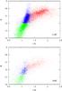 |
Fig. 8 K − J − K diagram for LMC and SMC red variables. |
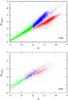 |
Fig. 9 EROS Wesenheit index vs. K magnitude, for LMC and SMC red variables. Wesenheit index is derived from EROS R and B magnitudes. |
4.4. The slope-J − K colour diagram
In the infrared, the C-rich stars appear systematically redder (J − K > 1.4) than O-rich stars (Frogel et al. 1990; Costa & Frogel 1996; Cioni et al. 2000a; Soszynski et al. 2005); however, in K vs. J − K diagrams (Fig. 8) there is some overlap between the C and O regions. The efficient way to separate the C and O stars is to combine the slope aV with the J − K colour. In the right panels of Fig. 4 we plot slope aV against J − K. Now separate clustering of C- and O-rich stars becomes more obvious. Based on this we propose the following criterion for C-rich stars:  (17)This criterion corresponds to the colour coding of stars in all panels in Fig. 4. Oxygen stars were separated from RGB and AGB using TRGB.
The Z-like shape of the distribution of stars in the aV − (J − K) panels in Fig. 4 represent the evolutionary sequence from O-rich RGB (top left) through O-rich AGB (right) down to C-rich AGB objects. For O-rich RGB stars, amplitudes tend to be low (left panels in Fig. 4) and slope parameter aV is poorly constrained. For higher luminosity O stars beyond TRGB, the slopes are better determined and stars concentrate around aV = 0.65 and J − K = 1.2. When TP-AGB begins and C-rich matter shows on the surface, the star migrates towards the inclined border line where there are stars with intermediate MS, S, and SC types. Eventually after crossing the border, it lands in the C-rich AGB star cluster. There is no appreciable difference between diagrams for the LMC and SMC. Using aV, K, and J − K we cannot only classify stars but also we could roughly determine its evolutionary stage. No such direct evolutionary interpretation was available for our slope parameter diagrams; however, this was made by resorting to cross identification of stars in the infrared and optical catalogues, and looking for which slope diagram concentrations correspond to the concentrations in the IR diagram.
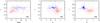 |
Fig. 10 Separation of C-rich, O-rich AGB, and red variables below the TRGB for LMC from OGLE LPV I and V photometry (Soszynski et al. 2005). The colour slope parameter aV vs. the amplitude of colour change (left panel). The colour slope parameter aV vs. K 2MASS magnitude (middle panel). Colour slope parameter vs. J − K colour (right panel). |
4.5. The Wesenheit index-luminosity relation
The Wesenheit index is a reddening-free parameter defined by a linear combination of stellar magnitudes. For EROS bands it could be calculated from the following equation (e.g. Tanvir 1997, and references there):  (18)where IEROS and VEROS are light curve average magnitudes (Sect. 3.1). For EROS, observations in both filters are simultaneous so time sampling yields no big uncertainty in colours.
Plots of WiEROS against the K magnitude for EROS LMC and SMC are presented in Fig. 9. Separation of C- and O-stars becomes particularly clear for the LMC. The location of three groups of stars with respect to the TRGB is visible in these plots. Similar diagrams for the Wesenheit index were already presented by Noda et al. (2002) and Soszyñski et al. (2009), but our filter bands and fields are rather different. In particular the accuracy of the estimation of the Wesenheit index is sensitive to the quality of the two-band coverage. For EROS the advantage stems from the simultaneous observation in two bands.
As the Wesenheit index is well correlated with K magnitude, it is in principle possible to implement the method of Sect. 4.3 by relying purely on EROS visual observations. In particular the Wesenheit index would be helpful to separate the RGB and AGB stars; however, such a classification would be less precise than than the one based on K luminosity. The gap on TRGB, clearly visible in K distribution, is hard to find in Wi. We can also separate RGB from AGB stars using the I-band. The TRGB appear at I = 14.54 in the LMC and I = 14.95 in the SMC (Cioni et al. 2000b).
4.6. OGLE
The bands employed by the EROS survey were non-standard. In this respect it is desirable to verify our results with OGLE observations obtained in the standard I and V bands. For the OGLE light curves, we performed the calculations similar to those for EROS. In this way we obtained values of the corresponding slope aV. The results for OGLE are presented in Fig. 10. We only plot LPV selected by Soszynski et al. (2005), who reject low-amplitude variables. Thus the number of stars with low colour amplitude and low K luminosity is lower than for EROS LMC.
Nevertheless, features revealed in Fig. 4 are present in Fig. 10. It is remarkable that, despite the small number of V observations and the interpolation of I magnitudes, separation of stars into respective classes is clear.
Soszynski et al. (2005) suggest that this sample should only contain the LPV AGB stars. We found that below the TRGB their stars follow the relation corresponding to the RGB stars. This may indicate that these stars belong to the AGB or at least that they follow the same relation as the RGB. These authors introduced the Period-Wesenheit index plots for a new method to differentiate between the O- and C-rich stars. Our method introduced in Sect. 4 is complementary as we use no information on periods. In this way our method is less demanding on time coverage of the light curves. Nevertheless, the two methods of selection of O- and C-rich stars are fairly consistent.
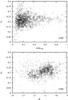 |
Fig. 11 Slope aV against V − R amplitude ampVR (top) and against 2MASS K magnitude, for MACHO LPV V and R photometry of the LMC. The C-rich stars are marked with circles. |
4.7. MACHO
The same procedure as for EROS was repeated for the MACHO data. MACHO uses non-standard filters fairly close to the standard V and R rather than V and I. In this way MACHO bands differ markedly from those of EROS and OGLE. This difference strongly affects our results for MACHO. The plots of the slope aV against either the colour amplitude for MACHO bands or the 2MASS K mag reveal no clear separation of the O- and C-rich stars in Fig. 11. This result seems consistent with the failure of the Wood et al. (2004) classification of the O- and C-rich stars based on similar filters. Thus our method only works for suitable photometric bands and is useless for MACHO photometry.
4.8. Maps of C/O ratio for Magellanic Clouds
In Table 1 we compared the three new methods described in Sects. 4.1, 4.3 and 4.4 with the well known method K(J − K) that uses J − K > 1.4 as a criterion for C-rich stars. Values in Table 1 were calculated only for variable stars. For all methods and for both Magellanic Clouds we found more C-rich stars than with the old method. The K(J − K) method yields the conclusion that the C/O ratio is much lower for the SMC than for the LMC. The aV(J − K) method yields the opposite result: the C/O ratio is greater in the SMC than in the LMC. Right panels of Fig. 4 shows that many C-rich stars lie between 1.15 and 1.4 on the J − K axis, especially for the LMC and aV(J − K) can separate stars without problem in this range of J − K. Different distributions of C-rich stars in the Magellanic Clouds probably depend on metallicity. Stars in the SMC are bluer than in the LMC for a similar stage of evolution.
Table 1 also contains results for aV(ampVI) and aV(K) methods. To compare aV(ampVI) with other methods, we divided O-rich stars to RGB and AGB stars using TRGB. Both methods are affected by overlapping O- and C-rich regions but still we found more C-rich stars than with the the K(J − K) method.
From our samples of O- and C-rich AGB stars from the aV(J − K) method, we calculated the C/O ratio in all cells belonging to a grid of 100′ × 100′ over the face of the LMC and grid of 45′ × 45′ over the face of the SMC. Figure 12 shows the ratios after boxcar average smoothing. A large hole in the central part of the SMC results from the lack of data in that sector. We retreive the same trends as described by Cioni & Habing (2003) in their Figs. 3 and 4: in the LMC the higher values of the C/O ratio are located in the outer regions, while the structure in the SMC is clumpier.
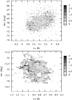 |
Fig. 12 Maps of the C/O ratio in the LMC (upper panel) and in the SMC (lower panel) obtained from EROS data using the aV(J − K) method described in Sect. 4.4. |
The C/O ratio for the MC’s from variable stars.
5. Clues to the underlying scenarios
Detailed modelling of the observed effect is beyond the scope of the present paper. As we pointed out above, modelling the late evolutionary stages is difficult and constitutes a whole branch of the theory. Worse, reconstruction of the synthetic spectra of C-rich AGB stars proved difficult and strongly relies on progress in the low-temperature opacities (Marigo et al. 2008). Simulation of the pulsations of the AGB stars is still more complex. The stellar atmosphere during pulses does not move uniformly up or down (Ireland et al. 2004b,a). Thus the non-linear pulsation model of a red giant is required to fit observations (Lebzelter & Wood 2005; Olivier & Wood 2005; Wood 2006).
However, it is possible that the effect demonstrated in Sect. 4 does not depend strongly on the details of the underlying physics. To demonstrate that we resorted to a crude and possibly non-physical model assuming that for all AGB stars during pulses dlog L /dlog Teff = const. and that the amplitude of variation in L and Teff remains the same for all stars. Thus any observed differences between stars would follow from a different response by their envelope to the same modulation. Next, we assume that the response of the upper envelope is quasi-static and may be determined by interpolation between different statics, i.e. non-pulsating, evolutionary models from different tracks but with the suitable L and Teff. This could be far from reality.
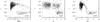 |
Fig. 13 Same as in Fig. 4 for the model slope parameter aV calculated for real LMC stars using Marigo et al. (2003) model sequences (see text for details). Our crude model yields a clear separation of O-rich RGB, O-rich AGB, and C-rich AGB stars. |
We employed the tracks calculated by Girardi & Marigo (2007) and available for download4 to interpolate properties of individual stars at their extreme luminosities. we take luminosity L, effective temperature Teff, absolute bolometric magnitude Mbol, absolute magnitudes in Johnson-Cousin-Glass UBVRIJHGK pass-bands, and surface carbon-to-oxygen number ratio C/O listed for the tracks. We interpolated these values to find how luminosities in filters vary with L and Teff during pulsation. In each track we identified the location of the RGB stars during TRGB and AGB phases of evolution. Next we perturbed their L and Teff to simulate the pulsation extreme phases. Using the corresponding filter magnitudes, we calculated slopes and amplitudes and plotted them in a similar way as for Fig. 4. By trial and error we found that a reasonable match with Fig. 4 is obtained for Δlog Teff = 0.042, Δlog L = 0.026, which leads to dlog L /dlog Teff = 0.614, but this works well for a wide range of both parameters. In this way we obtain Fig. 13 for the simulated data, where O- and C-rich stars separate in the slope-colour amplitude, slope-K luminosity and slope-colour J − K diagrams.
As our model is entirely artificial, we refrain from strong conclusions. However, this result should encourage theoreticians to reproduce our effect using fully realistic calculations (e.g. Marigo et al. 2008), and to use it to restrict the pulsation scenario.
6. Special properties of red variables
So far, our analysis has concerned the red variable stars with a modest amplitude (ampV < 1 mag), since they posed biggest classification problems. Also we payed no special attention to the multiperiodic variables in general and those with LSP in particular. Although our method for these stars does not explicitly account for their peculiarites, we briefly present results of its application hoping to provide additional clues missed in more specialised analyses.
6.1. Large-amplitude pulsations
In Fig. 14 we plot the slope- against colour amplitude for the whole range of amplitudes. This figure, which based on the raw data, corresponds exactly to the left column in Fig. 4, except for the extended amplitude scale. To illustrate here and in the next figure the relation of colour and luminosity amplitudes, ampVI and V, stars to the right of the line of inclination 0.6 passing through the origin are marked with different symbols. It appears that the pattern of the two populations of stars with small and large slopes discussed in Sect. 4 does extend to the large amplitudes, too. On a related plot of Wesenheit index vs. K luminosity, the large-amplitude C-rich stars appear redder, while the O-rich ones are bluer then the corresponding stars of small amplitude. We found no other peculiarities for the large-amplitude stars.
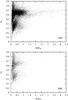 |
Fig. 14 Colour-slope parameter in function of amplitude of colour change for EROS LMC and SMC data. Crosses mark large-amplitude variables. |
6.2. Long secondary pulsations
Up to now we have analysed the raw data. However, many RGB variables reveal combinations of two periodic variations: a short one, presumably a radial pulsation, and a LSP. The corresponding periods form sequences B /B′ and D in the period- luminosity diagram (P-L). The nature of the LSP in RGB stars is still a mystery for interpretation (Soszyński (2007); Nicholls et al. (2009) and references therein). The D sequence periods are roughly ten times longer than the B ones and correspond to no known radial pulsation mode. The B sequence may correspond to a low-number overtone radial mode. LSP is observed among at least 25% of low mass RGB stars and typical red amplitudes ampR do not exceed 0.8 mag.
In this section we apply methods of Sect. 4 to the time-filtered light curves of all EROS LMC and SMC red variable stars, whether known to display an LSP or not. In the process we use the fact that our procedure does not require a known period. By employing the filters described in Sect. 3 we extracted separate light curves for fast and slow variations. The cut-off frequency of our filters depends on the mean magnitude to ensure a proper split of B and D sequences in systems known to display LSPs. Thus we obtain two different sets of amplitude and slope parameters ampV − short and ampV − long, aV − short and aV − long from respectively high- and low-pass filtered light curves.
In Fig. 15 we plot long-time amplitudes of variation of magnitude against short time ones, ampV − long vs. ampV − short for all EROS LMC and SMC data. Stars marked in Fig. 14 as possessing relatively large colour magnitude ampVI also exhibit absolutely large magnitudes ampV on at least one time scale. Although the amplitudes in Fig. 15 were estimated independently from two different light curves, they seem correlated. A consistent yet non-unique explanation would involve a similar mechanism for the short and long light variations.
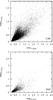 |
Fig. 15 Correlation between amplitudes of LSP and of shorter period variation for EROS LMC and SMC data. Crosses mark large-amplitude variables. |
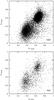 |
Fig. 16 Correlation between the colour slope parameter of LSPs and the shorter period for EROS LMC and SMC data. |
A stronger argument supporting the similarity of mechanisms of short and long time variations stems from the tight correlation of the short and long time scale slopes ashort and along revealed in Fig. 16. As discussed in Sect. 4 the two separate blobs in Fig. 16 correspond to C- and O-rich stars. The presence of just two such blobs rather than three or four at square vortices provides striking demonstration that short and long time scale variations both depend in the same way on surface chemical properties. Combined evidence from Figs. 15 and 16 indicates that both long and short time scale variations are due to the reaction of the stellar photosphere to similar kind of perturbations. We caution to not overinterpret this result. Firstly, our data contain both stars with and without known LSPs, and most light curves exhibit both periodic and irregular variations. However, it must be remembered that LSP amplitudes are not that small, and they are present in a sizable fraction of stars. If the LSP were produced away from the photosphere, one could expect to see some substructure within both C and O blobs in Fig. 16, so apparent lack of any internal structure in these blobs is consistent with LSPs being caused by the same kind of photosphere response as for the irregular variations and for the short period pulsations. In this context we stress that the EROS two-band observations are strictly simultaneous; hence our conclusions on photosphere evolution involve no interpolation or implicit light curve models.
7. Conclusions
A variable star during each cycle completes a closed loop on the colour-magnitude diagram. Non-periodic variables travel more involved routes. For each red variable star from the EROS survey, we derived a width and average slope of these figures, respectively ampVI and aV. In doing so, we benefitted from reliable colours obtained from EROS simultaneous two-band observations. In this way our analysis is less affected by variability and/or time sampling patterns. In particular, the gaps and aliasing pose no big problem for us as long as the data cover most of the pulsation period. This is a much less demanding requirement than a span of several cycles needed for reliable period analysis. The price paid in the process is a loss of any extra information; nevertheless, our analysis yields independent results that supplement more traditional period studies.
Our key method derived in Sect. 4.1 relies on the parameters aV and ampVI derived from pure visual observations. For its testing and verification we cross-referenced stellar positions from the EROS, OGLE and MACHO optical surveys with the infrared 2MASS catalogue. K magnitudes from the last catalogue were treated as indicators of stellar mean luminosity. Such a procedure is reliable for a known distance because it has little K band extinction and small bolometric correction for red variables. To completely free our optical luminosities from extinction, we employed the Wesenheit index. However, our key parameters result aV and ampVI are independent of distance and magnitude values. The range and correlation of two band magnitude changes are the only parameters that are important for us.
We demonstrated that in the aV and ampVI diagram, red variable stars form two well defined bands along aV = 0.4 and 0.65 lines. The bands occupied the same location for both the LMC and SMC stars. We argued that such a diagram constitutes a new method for differentiating of C- and O-rich RGB stars from purely visual observations. So far, effective photometric methods have relied on infrared observations. In fact, the dichotomy of C/O star distribution becomes even more prominent in the slope aV – K luminosity and slope – (J − K) colour diagrams for all stars from our sample. The clustering is particularly pronounced, both for LMC and SMC, in the slope-luminosity diagram. There the AGB and RGB stars separate well, apart from the usual C/O split of aV. In this particular diagram stellar evolutionary tracks RGB-TRGB-AGB(O)-AGB(C) are particularly well defined. While the detailed location of clusters in our diagnostic diagrams does depend on passbands, it is clearly manifested both for both EROS and OGLE two-band photometries. However, the bands employed by MACHO are not suitable to our classification method.
The final proof of the physical meaning of the clustering observed in our diagrams stems from the cross-check with catalogues of C-rich stars. The overwhelming majority of C-rich stars from catalogues by Kontizas et al. (2001), Groenewegen (2004), Rebeirot et al. (1993), Morgan & Hatzidimitriou (1995), for LMC and SMC, belongs to the low-aV slope cluster. Thus it appears that indeed the C- and O-rich stars belong to separate clusters in our aV vs. ampVI diagnostic diagram. In this way we discovered and verified a new method of distinguishing between C- and O-rich stars. Our method works for sparse coverage in two-colour light curves in the bands resembling V and I. Since we rely on colours, the measurements in both filters should be (nearly) simultaneous. Our method was tested successfully for EROS-2 LMC and SMC observations and also for OGLE data. It does not seem to suffer from any metallicity effect as cluster locations for the LMC and SMC were identical. Using simple simulations based on realistic evolutionary models of RGB, we demonstrated plausible cause of the effect revealed by our method; however, for as broad filters as those used by MACHO our method fails. One future application of our diagrams is to test the pulsation evolutionary models on a large population of RGB and AGB stars.
Using our method of differentiating the O- and C-rich stars we were able to derive the population C/O star ratio, an indicator of the mean metallicity of a stellar population, as well as a tracer of the history of stellar formation (Cioni et al. 2006). Our selection can recognise more C-rich stars than using J − K > 1.4 criterion, and it yields higher values of C/O ratio. Thus we were able to produce C/O maps for the LMC and SMC.
We payed some attention to colour correlation properties of the LSP compared to the short primary pulsation (SPP). Our results provide some evidence favouring origin of both LSP and SPP in the stellar photosphere. This follows from the correlation of colour-magnitude slopes and separately from correlation of amplitudes for the LSP and SPP. In other words, both SPP and LSP depend on the chemical (C/O) properties of the photosphere. The colour variations would be consistent with modulation of the effective temperature. This seems to exclude any aspect effects, e.g. eclipses, as a cause of LSP; however, using our purely photometric observations it would be premature to conclude that both SPP and LSP clocks are due to pulsation. However, both clocks should somehow affect the photosphere in similar ways.
Acknowledgments
We would like to thank Jim Rich for his careful reading of the manuscript and the anonymous referee for helpful comments. This work made use of EROS-2 data, which were kindly provided by the EROS collaboration. The EROS (Expérience de Recherche d’Objets Sombres) project was funded by the CEA and the IN2P3 and INSU CNRS institutes. We acknowledge use of data the Two Micron All Sky Survey, which is a joint project of the University of Massachusetts and the Infrared Processing and Analysis Center/California Institute of Technology, funded by the National Aeronautics and Space Administration and the National Science Foundation. This work was carried out, for A.S.C., J.P.B., J.B.M., and M.W., within the framework of the European Associated Laboratory “Astrophysics Poland-France”. A.S.C. acknowledges support by the Polish grant MNiSW N N203 3020 35.
References
- Afonso, C., Albert, J. N., Alard, C., et al. 2003, A&A, 404, 145 [NASA ADS] [CrossRef] [EDP Sciences] [Google Scholar]
- Alard, C., Blommaert, J. A. D. L., Cesarsky, C., et al. 2001, ApJ, 552, 289 [NASA ADS] [CrossRef] [Google Scholar]
- Alcock, C., Allsman, R. A., Alves, D., et al. 1997, ApJ, 486, 697 [NASA ADS] [CrossRef] [Google Scholar]
- Alcock, C., Allsman, R., Alves, D., et al. 2003, VizieR Online Data Catalog, 2247, [Google Scholar]
- Ansari, R. 1996, Vistas in Astronomy, 40, 519 [Google Scholar]
- Aubourg, E., Bareyre, P., Brehin, S., et al. 1995, A&A, 301, 1 [NASA ADS] [Google Scholar]
- Bergeat, J., Knapik, A., & Rutily, B. 2001, A&A, 369, 178 [NASA ADS] [CrossRef] [EDP Sciences] [Google Scholar]
- Bond, I. A., Abe, F., Dodd, R. J., et al. 2001, MNRAS, 327, 868 [NASA ADS] [CrossRef] [Google Scholar]
- Bowen, G. H., & Willson, L. A. 1991, ApJ, 375, L53 [NASA ADS] [CrossRef] [Google Scholar]
- Bressan, A., Chiosi, C., & Tantalo, R. 1996, A&A, 311, 425 [NASA ADS] [Google Scholar]
- Bruzual, G., & Charlot, S. 2003, MNRAS, 344, 1000 [NASA ADS] [CrossRef] [Google Scholar]
- Cioni, M.-R. L., & Habing, H. J. 2003, A&A, 402, 133 [NASA ADS] [CrossRef] [EDP Sciences] [Google Scholar]
- Cioni, M.-R., Loup, C., Habing, H. J., et al. 2000a, A&AS, 144, 235 [NASA ADS] [CrossRef] [EDP Sciences] [Google Scholar]
- Cioni, M.-R. L., Habing, H. J., & Israel, F. P. 2000b, A&A, 358, L9 [NASA ADS] [Google Scholar]
- Cioni, M.-R. L., van der Marel, R. P., Loup, C., & Habing, H. J. 2000c, A&A, 359, 601 [NASA ADS] [Google Scholar]
- Cioni, M.-R. L., Marquette, J.-B., Loup, C., et al. 2001, A&A, 377, 945 [NASA ADS] [CrossRef] [EDP Sciences] [Google Scholar]
- Cioni, M.-R. L., Blommaert, J. A. D. L., Groenewegen, M. A. T., et al. 2003, A&A, 406, 51 [Google Scholar]
- Cioni, M.-R. L., Girardi, L., Marigo, P., & Habing, H. J. 2006, A&A, 448, 77 [NASA ADS] [CrossRef] [EDP Sciences] [Google Scholar]
- Costa, E., & Frogel, J. A. 1996, AJ, 112, 2607 [NASA ADS] [CrossRef] [Google Scholar]
- Derekas, A., Kiss, L. L., Bedding, T. R., et al. 2006, ApJ, 650, L55 [NASA ADS] [CrossRef] [Google Scholar]
- Derue, F., Marquette, J.-B., Lupone, S., et al. 2002, A&A, 389, 149 [NASA ADS] [CrossRef] [EDP Sciences] [Google Scholar]
- Feast, M. W., Glass, I. S., Whitelock, P. A., & Catchpole, R. M. 1989, MNRAS, 241, 375 [NASA ADS] [CrossRef] [Google Scholar]
- Fisz, M. 1963, Probability Theory and Mathematical Statistics (New York: Wiley) [Google Scholar]
- Fraser, O. J., Hawley, S. L., Cook, K. H., & Keller, S. C. 2005, AJ, 129, 768 [NASA ADS] [CrossRef] [Google Scholar]
- Frogel, J. A., Mould, J., & Blanco, V. M. 1990, ApJ, 352, 96 [NASA ADS] [CrossRef] [Google Scholar]
- Girardi, L., & Marigo, P. 2007, in Why Galaxies Care About AGB Stars: Their Importance as Actors and Probes, ed. F. Kerschbaum, C. Charbonnel, & R. F. Wing, ASP Conf. Ser., 378, 20 [Google Scholar]
- Groenewegen, M. A. T. 2004, A&A, 425, 595 [NASA ADS] [CrossRef] [EDP Sciences] [Google Scholar]
- Groenewegen, M. A. T., & de Jong, T. 1993, A&A, 267, 410 [NASA ADS] [Google Scholar]
- Hoefner, S., Fleischer, A. J., Gauger, A., et al. 1996, A&A, 314, 204 [NASA ADS] [Google Scholar]
- Iben, Jr., I. 1981, ApJ, 246, 278 [NASA ADS] [CrossRef] [Google Scholar]
- Iben, Jr., I., & Renzini, A. 1983, ARA&A, 21, 271 [NASA ADS] [CrossRef] [Google Scholar]
- Ireland, M. J., Scholz, M., Tuthill, P. G., & Wood, P. R. 2004a, MNRAS, 355, 444 [NASA ADS] [CrossRef] [Google Scholar]
- Ireland, M. J., Scholz, M., & Wood, P. R. 2004b, MNRAS, 352, 318 [NASA ADS] [CrossRef] [Google Scholar]
- Ita, Y., Tanabé, T., Matsunaga, N., et al. 2004a, MNRAS, 353, 705 [NASA ADS] [CrossRef] [Google Scholar]
- Ita, Y., Tanabé, T., Matsunaga, N., et al. 2004b, MNRAS, 347, 720 [NASA ADS] [CrossRef] [Google Scholar]
- Izzard, R. G., Tout, C. A., Karakas, A. I., & Pols, O. R. 2004, MNRAS, 350, 407 [NASA ADS] [CrossRef] [Google Scholar]
- Kiss, L. L., & Bedding, T. R. 2003, MNRAS, 343, L79 [NASA ADS] [CrossRef] [Google Scholar]
- Kiss, L. L., & Bedding, T. R. 2004, MNRAS, 347, L83 [NASA ADS] [CrossRef] [Google Scholar]
- Kontizas, E., Dapergolas, A., Morgan, D. H., & Kontizas, M. 2001, A&A, 369, 932 [NASA ADS] [CrossRef] [EDP Sciences] [Google Scholar]
- Lançon, A., & Mouhcine, M. 2002, A&A, 393, 167 [NASA ADS] [CrossRef] [EDP Sciences] [Google Scholar]
- Lasserre, T., Afonso, C., Albert, J. N., et al. 2000, A&A, 355, L39 [NASA ADS] [Google Scholar]
- Lebzelter, T., & Hinkle, K. H. 2002, A&A, 393, 563 [NASA ADS] [CrossRef] [EDP Sciences] [Google Scholar]
- Lebzelter, T., & Wood, P. R. 2005, A&A, 441, 1117 [NASA ADS] [CrossRef] [EDP Sciences] [Google Scholar]
- Maraston, C. 1998, MNRAS, 300, 872 [NASA ADS] [CrossRef] [Google Scholar]
- Maraston, C. 2005, MNRAS, 362, 799 [NASA ADS] [CrossRef] [Google Scholar]
- Marigo, P., Girardi, L., & Bressan, A. 1999, A&A, 344, 123 [NASA ADS] [Google Scholar]
- Marigo, P., Girardi, L., & Chiosi, C. 2003, A&A, 403, 225 [NASA ADS] [CrossRef] [EDP Sciences] [Google Scholar]
- Marigo, P., Girardi, L., Bressan, A., et al. 2008, A&A, 482, 883 [NASA ADS] [CrossRef] [EDP Sciences] [Google Scholar]
- Matsunaga, N., Fukushi, H., & Nakada, Y. 2005, MNRAS, 364, 117 [NASA ADS] [CrossRef] [Google Scholar]
- Morgan, D. H., & Hatzidimitriou, D. 1995, A&AS, 113, 539 [NASA ADS] [Google Scholar]
- Mouhcine, M. 2002, A&A, 394, 125 [NASA ADS] [CrossRef] [EDP Sciences] [Google Scholar]
- Mouhcine, M., & Lançon, A. 2002, A&A, 393, 149 [NASA ADS] [CrossRef] [EDP Sciences] [Google Scholar]
- Mouhcine, M., & Lançon, A. 2003, MNRAS, 338, 572 [NASA ADS] [CrossRef] [Google Scholar]
- Nicholls, C. P., Wood, P. R., Cioni, M., & Soszyński, I. 2009, MNRAS, 399, 2063 [NASA ADS] [CrossRef] [Google Scholar]
- Noda, S., Takeuti, M., Abe, F., et al. 2002, MNRAS, 330, 137 [NASA ADS] [CrossRef] [Google Scholar]
- Noda, S., Takeuti, M., Abe, F., et al. 2004, MNRAS, 348, 1120 [NASA ADS] [CrossRef] [Google Scholar]
- Olivier, E. A., & Wood, P. R. 2005, MNRAS, 362, 1396 [NASA ADS] [CrossRef] [Google Scholar]
- Paczynski, B., Stanek, K. Z., Udalski, A., et al. 1994, unpublished [arXiv:astro-ph/9411004] [Google Scholar]
- Palanque-Delabrouille, N., Afonso, C., Albert, J. N., et al. 1998, A&A, 332, 1 [NASA ADS] [Google Scholar]
- Raimondo, G., Cioni, M.-R. L., Rejkuba, M., & Silva, D. R. 2005, A&A, 438, 521 [NASA ADS] [CrossRef] [EDP Sciences] [Google Scholar]
- Rebeirot, E., Azzopardi, M., & Westerlund, B. E. 1993, A&AS, 97, 603 [NASA ADS] [Google Scholar]
- Renzini, A., & Buzzoni, A. 1986, in Spectral evolution of galaxies, 195 [Google Scholar]
- Soszyński, I. 2007, ApJ, 660, 1486 [NASA ADS] [CrossRef] [Google Scholar]
- Soszynski, I., Udalski, A., Kubiak, M., et al. 2004a, Acta Astron., 54, 129 [NASA ADS] [Google Scholar]
- Soszynski, I., Udalski, A., Kubiak, M., et al. 2004b, Acta Astron., 54, 347 [NASA ADS] [CrossRef] [Google Scholar]
- Soszynski, I., Udalski, A., Kubiak, M., et al. 2005, Acta Astron., 55, 331 [NASA ADS] [Google Scholar]
- Soszyñski, I., Udalski, A., Szymañski, M. K., et al. 2009, Acta Astron., 59, 239 [NASA ADS] [Google Scholar]
- Tanvir, N. R. 1997, in The Extragalactic Distance Scale, ed. M. Livio, M. Donahue, & N. Panagia, 91 [Google Scholar]
- Tisserand, P., Le Guillou, L., Afonso, C., et al. 2007, A&A, 469, 387 [NASA ADS] [CrossRef] [EDP Sciences] [Google Scholar]
- Udalski, A., Kubiak, M., & Szymanski, M. 1997, Acta Astron., 47, 319 [NASA ADS] [Google Scholar]
- Wood, P. R. 1979, ApJ, 227, 220 [NASA ADS] [CrossRef] [Google Scholar]
- Wood, P. R. 2000, Pub. Astron. Soc. Austral., 17, 18 [Google Scholar]
- Wood, P. R. 2006, Mem. Soc. Astron. Ital., 77, 76 [NASA ADS] [Google Scholar]
- Wood, P. R., Alcock, C., Allsman, R. A., et al. 1999, in Asymptotic Giant Branch Stars, ed. T. Le Bertre, A. Lebre, & C. Waelkens, IAU Symp., 191, 151 [Google Scholar]
- Wood, P. R., Olivier, E. A., & Kawaler, S. D. 2004, ApJ, 604, 800 [NASA ADS] [CrossRef] [Google Scholar]
- Zebrun, K., Soszynski, I., Wozniak, P. R., et al. 2001, Acta Astron., 51, 317 [NASA ADS] [Google Scholar]
All Tables
All Figures
|
Fig. 1 Sample EROS light curves for two stars with spectral types assigned by Cioni et al. (2001): DCMC J052618.12-694100.0 of type C (top row) and DCMC J052446.91-694949.9 of type M (bottom row). The left, middle, and right panels present the raw, low-pass, and high-pass light curves, respectively. For details of filtering see Sect. 3.2 |
| In the text | |
|
Fig. 2 Sample plot of raw colour and magnitude variations for the same 2 stars as in Fig. 1. We also plot the regression lines. Their inclination parameter is aV, discussed in the text. |
| In the text | |
|
Fig. 3 Plot of the colour–magnitude correlation coefficient against the slope of magnitude-colour relation, for EROS LMC and SMC data. The correlation coefficient serves as a measure of quality of the slope av. The horizontal lines correspond to probability 0.995 of the null hypothesis H0, i.e. points lying above correspond to statistically significant correlation. |
| In the text | |
|
Fig. 4 Plots depicting three methods of distinguishing O- and C-rich variable stars (from left to right): slope-colour amplitude aV(ampVI), slope-K magnitude aV(K) and slope-J − K colour aV(J − K), for EROS LMC (top) and SMC (bottom) data. Vertical lines indicate adopted TRGB dividing RGB and AGB stars. See text for a detailed description of the methods and parameters of the boundaries. Black, dark grey, and light grey dots (blue, red, and green in electronic edition) respectively mark O- and C-rich AGB stars and O-rich RGB ones, classified using K magnitudes for AGB/RGB and leftmost panels for O/C content. |
| In the text | |
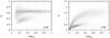 |
Fig. 5 Comparision of aV plot in Fig. 4 with that for aI. |
| In the text | |
|
Fig. 6 Similar plots as in Fig. 4 for C-rich, O-rich, and intermediate stars of Cioni et al. (2001), of respective spectral types C (triangles), M (circles), and S (squares). |
| In the text | |
|
Fig. 7 C-rich stars in LMC (upper panels) from Kontizas et al. (2001) and Groenewegen (2004) and in SMC (lower panels) from Rebeirot et al. (1993) and Morgan & Hatzidimitriou (1995). Colour-slope parameter aV in function of: amplitude of colour change ampVI (left panels); K 2MASS magnitude (middle panels); J − K colour (right panels). |
| In the text | |
|
Fig. 8 K − J − K diagram for LMC and SMC red variables. |
| In the text | |
|
Fig. 9 EROS Wesenheit index vs. K magnitude, for LMC and SMC red variables. Wesenheit index is derived from EROS R and B magnitudes. |
| In the text | |
|
Fig. 10 Separation of C-rich, O-rich AGB, and red variables below the TRGB for LMC from OGLE LPV I and V photometry (Soszynski et al. 2005). The colour slope parameter aV vs. the amplitude of colour change (left panel). The colour slope parameter aV vs. K 2MASS magnitude (middle panel). Colour slope parameter vs. J − K colour (right panel). |
| In the text | |
|
Fig. 11 Slope aV against V − R amplitude ampVR (top) and against 2MASS K magnitude, for MACHO LPV V and R photometry of the LMC. The C-rich stars are marked with circles. |
| In the text | |
|
Fig. 12 Maps of the C/O ratio in the LMC (upper panel) and in the SMC (lower panel) obtained from EROS data using the aV(J − K) method described in Sect. 4.4. |
| In the text | |
|
Fig. 13 Same as in Fig. 4 for the model slope parameter aV calculated for real LMC stars using Marigo et al. (2003) model sequences (see text for details). Our crude model yields a clear separation of O-rich RGB, O-rich AGB, and C-rich AGB stars. |
| In the text | |
|
Fig. 14 Colour-slope parameter in function of amplitude of colour change for EROS LMC and SMC data. Crosses mark large-amplitude variables. |
| In the text | |
|
Fig. 15 Correlation between amplitudes of LSP and of shorter period variation for EROS LMC and SMC data. Crosses mark large-amplitude variables. |
| In the text | |
|
Fig. 16 Correlation between the colour slope parameter of LSPs and the shorter period for EROS LMC and SMC data. |
| In the text | |
Current usage metrics show cumulative count of Article Views (full-text article views including HTML views, PDF and ePub downloads, according to the available data) and Abstracts Views on Vision4Press platform.
Data correspond to usage on the plateform after 2015. The current usage metrics is available 48-96 hours after online publication and is updated daily on week days.
Initial download of the metrics may take a while.