| Issue |
A&A
Volume 529, May 2011
|
|
|---|---|---|
| Article Number | A57 | |
| Number of page(s) | 5 | |
| Section | Astronomical instrumentation | |
| DOI | https://doi.org/10.1051/0004-6361/201116566 | |
| Published online | 01 April 2011 | |
Research Note
Characterisation of the CAFOS linear spectropolarimeter⋆
1 European Organization for Astronomical Research in the Southern Hemisphere (ESO), Karl-Schwarzschild-Str. 2, 85748, Garching b. München, Germany
e-mail: This email address is being protected from spambots. You need JavaScript enabled to view it.
2 Max-Planck-Institut für Astrophysik, Karl-Schwarzschild-Str. 1, 85741 Garching b. München, Germany
Received: 24 January 2011
Accepted: 9 February 2011
Abstract
Aims. We present a full analysis of the CAFOS polarimeter mounted at the Calar Alto 2.2 m telescope. This provides future users of this mode with all necessary information to properly correct for instrumental effects in polarization data obtained with this instrument.
Methods. The standard stars BD+59d389 (polarized) and HD 14069 (unpolarized) were observed with CAFOS in November, 2010, using 16 half-wave plate angles. The linear spectropolarimetric properties of CAFOS were studied using a Fourier analysis of the resulting data.
Results. CAFOS shows a roughly constant instrumental polarization at the level of ~0.3% between 4000 Å and 8600 Å. Below 4000 Å, the spurious polarization grows to reach ~0.7% at 3600 Å. This instrumental effect is most likely produced by the telescope optics, and appears to be additive. The Wollaston prism clearly operates less than ideally. However, the problem is largely removed by using at least four retarder plate angles. The chromatism of the half-wave plate causes a peak-to-peak oscillation of ~11 degrees in the polarization angle. This can be effectively corrected using the tabulated values presented in this paper. The Fourier analysis shows that the k ≠ 0,4 harmonics are practically negligible between 3800 and 7400 Å.
Conclusions. After correcting for instrumental polarization and retarder plate chromatism, with four half-wave plate angles CAFOS can reach an rms linear polarization accuracy of about 0.1%.
Key words: techniques: polarimetric / instrumentation: polarimeters
Based on observations collected at the German-Spanish Astronomical Center, Calar Alto, jointly operated by the Max-Planck-Institut für Astronomie Heidelberg and the Instituto de Astrofisica de Andalucia (CSIC).
© ESO, 2011
1. Introduction
While observing the bright supernova 2010jl, we obtained spectropolarimetry of this object using the Calar Alto Faint Object Spectrograph (CAFOS), mounted at the 2.2 m telescope in Calar Alto, Spain (Meisenheimer 1998). The results were published in Patat et al. (2010). The polarimetric mode of CAFOS has not been used extensively, and mostly in imaging mode (see Greiner et al. 2003, for an example). As we could not find a proper characterisation of the instrumental effects in the literature, during the campaign on SN 2010jl we ran a full analysis of the instrument. This is presented here with the aim of making it available to a wider community, who might find it useful for future spectropolarimetric observations with this instrument.
Dual-beam polarimeters such as CAFOS are composed of a half-wave retarder plate (HWP) followed by an analyzer, which is a Wollaston prism (WP) producing two beams with orthogonal directions of polarization, usually indicated as ordinary (O) and extraordinary (E) beams. With this instrumental setup, the Stokes parameters Q and U are derived by measuring the intensities in the O and E beams (fO,i, fE,i) at a given set of HWP angles θi (for a general overview, see Patat & Romaniello 2006 and references therein).
This is typically achieved through the normalized flux differences Fi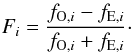 For an ideal polarimeter, the normalized flux differences obey the relation: Fi = Pcos(4θi − 2χ), where
  is the polarization degree and
  is the polarization position angle. Although any set of angles θi is in principle suitable for obtaining Q and U, the optimal choice is
  . In these conditions, one has that
where N is the number of HWP angles. Since Fi can be regarded as a co-sinusoidal signal modulated by the rotation of the HWP with a fundamental period 2π, these can be rewritten as a Fourier series (see Fendt et al. 1996): ![Mathematical equation: \begin{equation} F_i = a_0 + \sum_{k=1}^{N/2} \left [ a_k \cos \left( k \frac{2\pi i}{N}\right) + b_k \sin \left( k \frac{2\pi i}{N}\right) \right], \end{equation}](/articles/aa/full_html/2011/05/aa16566-11/aa16566-11-eq18.png) (1)where ak and bk are the Fourier coefficients. The Fourier analysis is particularly useful when N = 16; under these circumstances, the polarization signal is carried by the k = 4 component. In an ideal system, all other components are zero. Therefore, non-null Fourier coefficients for k ≠ 4 signal possible problems in the polarimeter. For the meaning of the various components the reader is referred to Fendt et al. (1996).
(1)where ak and bk are the Fourier coefficients. The Fourier analysis is particularly useful when N = 16; under these circumstances, the polarization signal is carried by the k = 4 component. In an ideal system, all other components are zero. Therefore, non-null Fourier coefficients for k ≠ 4 signal possible problems in the polarimeter. For the meaning of the various components the reader is referred to Fendt et al. (1996).
2. Observations and data reduction
The observations were carried out with CAFOS (Meisenheimer 1998). For this multi-mode instrument equipped with a 2K × 2K SITe-1d CCD (24 μm pixels, 0.53 arcsec/pixel), polarimetry is performed by introducing into the optical path a WP (18′′ throw) and a super-achromatic HWP, between the collimator and the grism. For our study, we observed the polarized star BD+59d389 (P(V) = 6.70 ± 0.02%, χ = 98.1 degrees; Schmidt et al. 1992) and the unpolarized star HD 14069 (P(V) = 0.02 ± 0.02%; Schmidt et al. 1992) on 2010, November 18.8 UT. All spectra were obtained with the low-resolution B200 grism coupled with a 1.0 arcsec slit, giving a spectral range 3300 − 8900 Å, a dispersion of ~ 4.7 Å px-1, and a FWHM resolution of 14.0 Å. The slit was aligned along the N-S direction. To enable the Fourier analysis up to the eight harmonic, we used N = 16 half-wave plate angles (0, 22.5, ..., 337.5). The exposure times were 180 s per HWP angle for both standard stars.
Data were bias and flat-field corrected, and wavelength calibrated using standard tasks within IRAF1. The Fourier analysis was carried out using specific routines written by ourselves.
3. Instrumental polarization
To characterize the instrumental polarization of CAFOS, we first analyzed the data obtained for the unpolarized standard star. The result of the Fourier analysis is presented in Fig. 1 for a 200 Å wide bin centered on 5500 Å. The normalized flux differences show a marked modulation (upper panel), which is closely reproduced by a sinusoidal function. The power spectrum (lower panel) displays a distinctive peak at the k = 4 overtone, corresponding to a linear polarization signal (see Sect. 1), reaching P = 0.26% (the k = 0 term is also non-null, but we discuss this in Sect. 4). The fact that the signal is modulated by the retarder plate rotation implies that the source of instrumental polarization precedes the HWP along the optical path. Therefore, the observed polarization most likely arises within the collimator and/or the telescope mirrors. For instance, inhomogeneities in the mirror coatings can break the circular symmetry, leading to an incomplete cancellation of the linear polarization generated by reflections (see Tinbergen 1996 and Leroy 2000 for general introductions to the subject). Such a system would behave as a partial polarizer, characterized by a certain position angle (χins) that does not depend on wavelength, but only on the geometry of the system asymmetry. In general, the effect of the instrumental polarization depends on the Stokes vector that characterizes the input signal, which makes the correction of instrumental polarization particularly difficult. However, when the instrumental polarization is much smaller than 1, the effect is additive, and the spurious signal can be removed by subtracting it vectorially from the measured one (see for instance Patat & Romaniello 2006 for the case of VLT-FORS1).
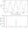 |
Fig. 1 Fourier analysis applied to the unpolarized standard star HD 14069 at 5500 Å (200 Å bin). Top: normalized flux differences. The curves trace the partial reconstruction using eight harmonics (solid) and the fourth harmonic only (dotted). The dashed horizontal line is placed at the average of the F values (a0). Bottom: harmonics power spectrum. The dashed line indicates the 5-σ level of the uncertainty. |
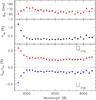 |
Fig. 2 CAFOS instrumental polarization. Upper panel: instrumental polarization position angle. The dashed line indicates the average value. Mid panel: instrumental polarization degree. Lower panel: instrumental Stokes parameters. The dashed lines indicate the average value of Q and U in the wavelength range 4000–8600 Å, while the dotted lines mark the ± 0.05% deviations from the average value. |
A constant position angle is confirmed by the Fourier analysis applied across the whole wavelength range covered by our observations. In Fig. 2, we present the values of Qins and Uins derived within 200 Å wide bins between 3400 and 8600 Å (lower panel), and the implied position angle χins (upper panel). The average value of χins is 166.3 degrees, and the rms deviation of the single measurements is 3.6 degrees. The smooth oscillation seen in the position angle is related to the chromatism of the HWP retardance (see Sect. 5). As far as the polarization is concerned, this reaches 0.74 ± 0.08% at 3400 Å, and rapidly decreases to 0.33 ± 0.01% at 4000 Å, remaining constant to within 0.05% up to 8600 Å. The reason for the marked increase seen bluewards of 4000 Å is unclear, but it might be related to the decrease in the efficiency of the anti-reflexion coatings of the collimator lenses.
The average values of the instrumental Stokes parameters above 4000 Å are ⟨ Qins ⟩ = + 0.25 ± 0.03%, and ⟨ Uins ⟩ = −0.13 ± 0.03%, leading to an average polarization of Pins = 0.28 ± 0.03%. The wavelength range below 3800 Å is affected by other instrumental problems that make it hardly usable with the typical set of four HWP angles (see next section). Therefore, this constant correction is sufficient to guarantee the removal of the instrumental polarization with a maximum error of 0.05%, which is comparable to the maximum accuracy one can reach with CAFOS with four HWP angles (see next section).
We note that the instrumental polarization correction derived here is strictly valid only for an object placed on the CAFOS reference pixel used for the acquisition onto the 1.0 arcsec slit. With the present analysis, we cannot exclude position-dependent effects, as is also the case for the FORS instruments (Patat & Romaniello 2006).
4. Fourier analysis
For the Fourier analysis of the CAFOS polarimetric performances, we have used the data obtained for the polarized standard star. Figure 3 shows an example for a 200 Å wide bin centered on 5500 Å. The only components with statistically significant power are k = 0 and k = 4; there is a hint of a non-null k = 2 component, which is related to the so-called pleochroism (Fendt et al. 1996; Patat & Romaniello 2006), but this is only marginally significant at the 5-σ level. The original signal can be reconstructed using only the k = 4 harmonic, with maximum residuals ΔFi of ~ 0.1%. This implies that four HWP angles are sufficient to the derive Stokes parameters with a maximum error of this order. The polarization degree derived using 16 HWP angles at 5500 Å is 6.43 ± 0.01%. After applying the instrumental polarization correction described in the previous section, this value becomes 6.6 ± 0.1%. This is fully consistent with the reference value 6.70 ± 0.02% measured in the V passband (Schmidt et al. 1992).
In the example illustrated in Fig. 3, we find that a0 = 1.88 ± 0.01% (the corresponding value derived from the unpolarized standard is 1.93 ± 0.01%; see also Fig. 1, upper panel). This indicates that the WP deviates from the ideal case, in that an unpolarized incoming beam is not divided precisely into two identical fractions (see Patat & Romaniello 2006, their Sect. 7). As a consequence, using only two HWP angles (which is the minimum set needed to fully reconstruct the Stokes vector) would lead to a very significant error in the final result.
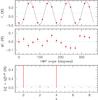 |
Fig. 3 Fourier analysis applied to the polarized standard star BD+59d389 at 5500 Å (200 Å bin). Top: normalized flux differences. The curves trace the partial reconstruction using eight harmonics (solid) and the fourth harmonic only (dotted). The dashed horizontal line is placed at the average of the F values (a0). Middle: residuals from the reconstruction using the k = 4 harmonic. Bottom: harmonics power spectrum. The dashed line indicates the 5-σ level uncertainty. |
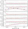 |
Fig. 4 Power spectrum of the first six harmonics as a function of wavelength (ordinate scale is in %). The solid thin lines trace the 5-σ confidence level. The filled squares in the k = 4 plot are the broad-band polarization measurements by Schmidt et al. (1992). |
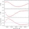 |
Fig. 5 Instrumental polarization corrected Stokes parameters Q (top panel) and U (mid panel) for BD+59d389. The bottom panel shows the phase retardance variation as a function of wavelength. |
To study the instrumental performance as a function of wavelength, we ran the same analysis within 200 Å wide bins between 3400 and 8600 Å. The result for the first six harmonics is shown in Fig. 4. The k = 0 component is always significant, exceeding ~3% at 7500 Å, but this is fairly well corrected if the data set includes at least four HWP positions. As for components k = 1 and 2, these are detected at a significant level below 3800 Å and above 7000 Å. At 3600 Å, the usage of four HWP angles leads to errors larger than 0.3%, making data bluewards of 3800 Å hardly usable. At the red edge, deviations are smaller than 0.2% bluewards of 7400 Å, while they can exceed 0.3% above 8200 Å.
As the k = 4 component of the power spectrum is the linear polarization degree, its wavelength dependence can be directly compared to the broad-band values available in the literature (Schmidt et al. 1992). These are overplotted in the k = 4 panel of Fig. 4 (filled squares). As expected based on the estimates of the instrumental polarization (see Sect. 3), there is a difference of about 0.3% above 4000 Å. The value corresponding to the U passband shows a larger deviation (0.7%), which is consistent with the increase in the instrumental polarization seen below 4000 Å (see Fig. 2). We note that, as the polarization signals of the star and the instrument are close to orthogonal, the corrected value is higher than the measured one.
5. HWP chromatism
Although the retarder plate deployed in CAFOS is super-achromatic, the phase retardance is expected to deviate from an ideal behavior as a function of wavelength. To quantify this effect, we used the polarized standard as reference. For this star, the polarization position angle is constant to within 0.1 degrees in the UBVRI domain, the average value being χ0 = 98.2 ± 0.1 degrees (Schmidt et al. 1992). Therefore, if Qobs and Uobs are the measured Stokes parameters, the phase retardance variation across the wavelength range can be computed as Δχ = χ − χ0, where ![Mathematical equation: \hbox{$\chi=\frac{1}{2}\arctan [(U_{\rm obs}-U_{\rm ins})/(Q_{\rm obs}-Q_{\rm ins})]$}](/articles/aa/full_html/2011/05/aa16566-11/aa16566-11-eq57.png) . The result is plotted in Fig. 5, and the values listed in Table 1.
. The result is plotted in Fig. 5, and the values listed in Table 1.
With these values at hand, the corrected Stokes parameters Qc and Uc can be obtained by the rotation:  where Q and U are the instrumental polarization-corrected Stokes parameters. Alternatively, the position angle obtained from Q and U can be corrected by subtracting Δχ.
The zero-point of the HWP angle is usually set so that θ = 0 corresponds to a null astronomical position angle in the plane of the sky around the central wavelength. This is not the case in CAFOS, as the deviation at 6000 Å is about 5.5 degrees, and is never zero between 3600 and 8600 Å (Fig. 5, bottom panel). However, given the way we computed Δχ, this correction provides position angles in the plane of the sky, where χ = 0 corresponds to the N-S direction.
6. Conclusions
We have presented a full analysis of the linear polarization properties of CAFOS. Although the instrument appears to be affected by a significant spurious polarization, this can be removed to within ~0.1%. The effect appears to be additive, and can therefore be easily corrected by vectorially subtracting the instrumental component in the Stokes Q,U plane.
As is typical of other dual-beam polarimeters (see for instance the case of FORS1, Patat & Romaniello 2006), the Wollaston prism is found to depart from the ideal case. In the worst case, the fraction of light in the ordinary and extraordinary beams for an unpolarized incoming signal deviates by ~2% from the theoretical 50/50 ratio. However, this defect is largely removed by the adoption of four retarder plate angles during the observations. Using the minimum set (two HWP angles) leads to large errors, especially in the case of low polarizations (~1%), and is therefore strongly discouraged.
The Fourier analysis shows that all harmonics with k ≠ 0, 4 are negligible in the wavelength range 3800–7400 Å, where a rms accuracy of 0.1% can be reached with a sufficient signal-to-noise ratio. This can be considered as the instrumental limit attainable with CAFOS with four HWP angles, within this spectral range. Below 3800 Å, the polarimetric properties rapidly degrade, requiring a larger number of HWP angles. The same applies, though to a smaller extent, to the region redwards of 8200 Å.
HWP retardance variation as a function of wavelength.
In this work, we have used data obtained with the B200 grism. Because of its tilted surfaces, the grism can act as a poor linear polarizer. Since in CAFOS this is placed after the analyzer, the spurious polarization produced by transmission is not modulated by the HWP rotation, and hence is effectively removed by the redundancy in the retarder-plate positions (see Patat & Romaniello 2006). The precise effect produced by the grism depends on its properties. However, the conclusions reached in this paper do not depend on the grism, provided that the data are obtained using at least four HWP angles.
In general, CAFOS appears to be perfectly suitable for linear polarization studies aiming at accuracies of a few 0.1%, making it a valid instrument for bright objects. As a term of reference, an accuracy of ~0.1% per resolution element (~50 Å) was reached for SN 2010jl (V ~ 13.5), with four exposures of 40 min each (Patat et al. 2010).
IRAF is distributed by the National Optical Astronomy Observatories, which are operated by the Association of Universities for Research in Astronomy, under contract with the National Science Foundation.
Acknowledgments
We wish to thank the personnel at Calar Alto Observatory for obtaining the extra calibrations required for the full polarimetric characterisation of CAFOS. This work has been done in the framework of the European
Large Collaboration Supernova Variety and Nucleosynthesis Yields (http://graspa.oapd.inaf.it/), whose members are acknowledged.
References
- Fendt, C., Beck, R., Lesch, H., & Neninger, N. 1996, A&A, 308, 713 [NASA ADS] [Google Scholar]
- Greiner, J., Klose, S., Reinsch, K., et al. 2003, Nature 426, 157 [NASA ADS] [CrossRef] [PubMed] [Google Scholar]
- Leroy, J. L. 2000, Polarization of light and astronomical observations (Singapore: Gordon & Breach) [Google Scholar]
- Meisenheimer, K. 1998, User Guide to the CAFOS 2.2 [Google Scholar]
- Patat, F., & Romaniello, M. 2006, PASP, 118, 146 [NASA ADS] [CrossRef] [Google Scholar]
- Patat, F., Taubenberger, S., Benetti, S., Pastorello, A., & Haryutyunian, A. 2010, A&A, 526, L6 [Google Scholar]
- Schmidt, G. D., Elston, R., & Lupie, O. L. 1992, AJ, 104, 1563 [NASA ADS] [CrossRef] [Google Scholar]
- Tinbergen, J. 1996, Astronomical polarimetry (Cambridge: Cambridge Univ. Press) [Google Scholar]
All Tables
All Figures
|
Fig. 1 Fourier analysis applied to the unpolarized standard star HD 14069 at 5500 Å (200 Å bin). Top: normalized flux differences. The curves trace the partial reconstruction using eight harmonics (solid) and the fourth harmonic only (dotted). The dashed horizontal line is placed at the average of the F values (a0). Bottom: harmonics power spectrum. The dashed line indicates the 5-σ level of the uncertainty. |
| In the text | |
|
Fig. 2 CAFOS instrumental polarization. Upper panel: instrumental polarization position angle. The dashed line indicates the average value. Mid panel: instrumental polarization degree. Lower panel: instrumental Stokes parameters. The dashed lines indicate the average value of Q and U in the wavelength range 4000–8600 Å, while the dotted lines mark the ± 0.05% deviations from the average value. |
| In the text | |
|
Fig. 3 Fourier analysis applied to the polarized standard star BD+59d389 at 5500 Å (200 Å bin). Top: normalized flux differences. The curves trace the partial reconstruction using eight harmonics (solid) and the fourth harmonic only (dotted). The dashed horizontal line is placed at the average of the F values (a0). Middle: residuals from the reconstruction using the k = 4 harmonic. Bottom: harmonics power spectrum. The dashed line indicates the 5-σ level uncertainty. |
| In the text | |
|
Fig. 4 Power spectrum of the first six harmonics as a function of wavelength (ordinate scale is in %). The solid thin lines trace the 5-σ confidence level. The filled squares in the k = 4 plot are the broad-band polarization measurements by Schmidt et al. (1992). |
| In the text | |
|
Fig. 5 Instrumental polarization corrected Stokes parameters Q (top panel) and U (mid panel) for BD+59d389. The bottom panel shows the phase retardance variation as a function of wavelength. |
| In the text | |
Current usage metrics show cumulative count of Article Views (full-text article views including HTML views, PDF and ePub downloads, according to the available data) and Abstracts Views on Vision4Press platform.
Data correspond to usage on the plateform after 2015. The current usage metrics is available 48-96 hours after online publication and is updated daily on week days.
Initial download of the metrics may take a while.