| Issue |
A&A
Volume 529, May 2011
|
|
|---|---|---|
| Article Number | A146 | |
| Number of page(s) | 16 | |
| Section | Interstellar and circumstellar matter | |
| DOI | https://doi.org/10.1051/0004-6361/201016228 | |
| Published online | 21 April 2011 | |
Ion irradiation of carbonaceous interstellar analogues
Effects of cosmic rays on the 3.4 μm interstellar absorption band
1
Institut d’Astrophysique Spatiale (IAS, UMR8617), CNRS; Univ
Paris-Sud,
bât. 121,
91405
Orsay,
France
e-mail: This email address is being protected from spambots. You need JavaScript enabled to view it.
2
Institut des Sciences Moléculaires d’Orsay (ISMO, UMR8214), CNRS;
Univ Paris-Sud, bât.
210, 91405
Orsay,
France
3
Institut de Physique Nucléaire d’Orsay (IPN, UMR8608), CNRS; Univ
Paris-Sud, bât.
102, 91405
Orsay,
France
4
Centre de Spectrométrie Nucléaire et de Spectrométrie de Masse
(CSNSM, UMR8609), CNRS; Univ Paris-Sud, bât. 104, 91405
Orsay,
France
Received:
29
November
2010
Accepted:
17
March
2011
Abstract
Context. A 3.4 μm absorption band (around 2900 cm-1), assigned to aliphatic C-H stretching modes of hydrogenated amorphous carbons (a-C:H), is widely observed in the diffuse interstellar medium, but disappears or is modified in dense clouds. This spectral difference between different phases of the interstellar medium reflects the processing of dust in different environments. Cosmic ray bombardment is one of the interstellar processes that make carbonaceous dust evolve.
Aims. We investigate the effects of cosmic rays on the interstellar 3.4 μm absorption band carriers.
Methods. Samples of carbonaceous interstellar analogues (a-C:H and soot) were irradiated at room temperature by swift ions with energy in the MeV range (from 0.2 to 160 MeV). The dehydrogenation and chemical bonding modifications that occurred during irradiation were studied with IR spectroscopy.
Results. For all samples and all ions/energies used, we observed a decrease of the aliphatic C-H absorption bands intensity with the ion fluence. This evolution agrees with a model that describes the hydrogen loss as caused by the molecular recombination of two free H atoms created by the breaking of C-H bonds by the impinging ions. The corresponding destruction cross section and asymptotic hydrogen content are obtained for each experiment and their behaviour over a large range of ion stopping powers are inferred. Using elemental abundances and energy distributions of galactic cosmic rays, we investigated the implications of these results in different astrophysical environments. The results are compared to the processing by UV photons and H atoms in different regions of the interstellar medium.
Conclusions. The destruction of aliphatic C-H bonds by cosmic rays occurs in characteristic times of a few 108 years, and it appears that even at longer time scales, cosmic rays alone cannot explain the observed disappearance of this spectral signature in dense regions. In diffuse interstellar medium, the formation by atomic hydrogen prevails over the destruction by UV photons (destruction by cosmic rays is negligible in these regions). Only the cosmic rays can penetrate into dense clouds and process the corresponding dust. However, they are not efficient enough to completely dehydrogenate the 3.4 μm carriers during the cloud lifetime. This interstellar component should be destroyed in interfaces between diffuse and dense interstellar regions where photons still penetrate but hydrogen is in molecular form.
Key words: cosmic rays / dust, extinction / evolution / methods: laboratory / infrared: ISM / ISM: lines and bands
Present address: Laboratory Astrophysics Group of the Max Planck Institute for Astronomy at the Friedrich Schiller University Jena, Institute of Solid State Physics, Helmholtzweg 3, 07743 Jena, Germany.
© ESO, 2011
1. Introduction
Interstellar dust continuously interacts with its surrounding environment. Its chemical and physical composition is determined by processes active in space, such as exposure to heat, shocks, H atoms, UV photons, and cosmic rays. The equilibrium between formation and destruction processes varies within each phase of the interstellar medium (ISM). Laboratory simulations of dust processing in conditions close to those of the interstellar medium may help to understand the evolution of carbonaceous interstellar matter components and to investigate the continuous cycle of organic matter between diffuse and dense regions of the interstellar medium. Infrared spectroscopy is a powerful tool to probe the transformations that are undergone in the different environments of the ISM.
The 3.4 μm absorption band (around 2900 cm-1) is one of the primary carbonaceous dust IR signatures observed in the ISM. This band corresponds to the C-H bond vibrations, and in particular to the stretching modes in the methyl (CH3) and methylene (CH2) groups. It is associated with the corresponding bending modes at 6.85 μm (1460 cm-1) and 7.25 μm (1380 cm-1). These aliphatic C-H IR absorption bands are widely observed in diffuse interstellar medium in the Milky Way and other galaxies (Wickramasinghe & Allen 1980; Adamson et al. 1990; Sandford et al. 1991; Pendleton et al. 1994; Whittet et al. 1997; Pendleton & Allamandola 2002; Spoon et al. 2004; Dartois et al. 2007). Hydrogenated amorphous carbons (a-C:H, also known as HAC in the astrophysical literature) have proven to be good analogues for this aliphatic interstellar dust component through identical IR spectral signatures (Dartois et al. 2005; Chiar et al. 2000).
Although dust is cycling between the different phases of the ISM and although this aliphatic hydrocarbon component is ubiquitous in diffuse ISM, the only absorption observed in this range in dense clouds is a large featureless band at 3.47 μm whose shape is different from the 3.4 μm band observed in diffuse ISM. This 3.47 μm band correlates with water ice. Its origin and attribution is still debated (Allamandola et al. 1993; Chiar et al. 1996; Brooke et al. 1999; Dartois & d’Hendecourt 2001; Dartois et al. 2002; Mennella 2010). The recent work of Bottinelli et al. (2010) seems to confirm that this band could coincide with the presence of ammonia hydrate in ice. The widespread distribution of the 3.4 μm band in the diffuse interstellar medium and its apparent disappearance or modification in dense clouds give constraints for understanding the formation and evolution of the interstellar aliphatic component. The effects of interstellar processing on this important carbonaceous dust component need to be investigated.
Irradiation by galactic cosmic rays (CR) is one of the interstellar processes known to destroy aliphatic C-H bonds, and this induces a decrease of the 3.4 μm band intensity. Cosmic rays are composed of highly energetic ions and electrons. Numerous works have been devoted to the study of energetic ions effect on hydrogenated carbonaceous matter by different diagnostic tools such as infrared or Raman spectroscopy, or techniques allowing one to measure the hydrogen content (e.g., Baumann et al. 1987; Prawer et al. 1987; González-Hernández et al. 1988; Fujimoto et al. 1988; Ingram & McCormick 1988; Zou et al. 1988; Adel et al. 1989; Marée et al. 1996; Pawlak et al. 1997; Som et al. 1999; Baptista et al. 2004; Som et al. 2005; Brunetto et al. 2009). It is observed that the irradiation of these materials results in a decrease of the aliphatic C-H spectral signatures and of the hydrogen content. The astrophysical implications of these laboratory simulations of hydrogenated carbon dust have been investigated by Mennella et al. (2003). The experiments were performed using 30 keV He+ ions. The effects of other ions and energies (in particular higher energies that are more similar to those of CR) have only been extrapolated. The authors have only considered protons of 1 MeV energy to represent the whole cosmic ray elements and energies (i.e., the approximation of 1 MeV monoenergetic protons). With the present work, we aim at performing a comprehensive study of the effect of cosmic rays on the interstellar aliphatic C-H features by combining the results of experiments conducted with a wide range of swift (i.e., energetic) ions and the use of a model describing the effective dehydrogenation of the irradiated material.
We report laboratory experiments aimed at studying energetic ion irradiation of interstellar dust analogues. The different hydrogenated carbonaceous analogue samples are presented in Sect. 2, followed by a description of the irradiation set-up. The experimental results are presented in Sect. 3. They are then implemented in an astrophysical context and discussed in Sect. 4. The conclusions are summarised in Sect. 5.
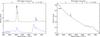 |
Fig. 1 Infrared spectra (before irradiation) of the different a-C:H and soot samples: IR spectra of samples a-C:H 1 (thickness d ≈ 10 μm) and a-C:H 2 (d ≈ 7 μm) are in the left panel and the soot IR spectrum is in the right panel (d ≈ 5 μm). Spectrum of a-C:H 1 is offset by 1.5 for a better clarity. |
2. Experiments
2.1. Samples production
Two different types of analogues of carbonaceous interstellar matter are produced for this study: hydrogenated amorphous carbons (a-C:H or HAC) and carbon soots.
The a-C:H samples were produced at the Institut d’Astrophysique Spatiale (Orsay, France) using a plasma-enhanced chemical vapour deposition (PECVD) system: a microwave-induced plasma of hydrocarbon precursor gas is created in a vacuum chamber (pressure maintained at approximatively 10-2 mbar) via an Evenson cavity coupled to a 2.45 GHz radio-frequency microwave generator. The precursor gas used is either methane or butadiene. The radicals and ions from the plasma are deposited on a substrate (KBr or KCl), which is located a few centimetres from the plasma, during a few minutes to approximately one hour depending on the experimental conditions. The few micrometer thick a-C:H film obtained can then be analysed ex situ.
The experiment “Nanograins” of the Institut des Sciences Moléculaires d’Orsay (France) allows us to produce the second kind of carbonaceous materials, hereafter named soot. Incomplete combustion reactions in a fuel-rich, premixed and low pressure (70 mbar) flame nucleate many polycyclic aromatic hydrocarbons and three dimensional soots. For a more detailed description, see Pino et al. (2008). A KBr substrate is placed in front of the flame extraction cone to retrieve the condensable phase. As a result, we obtain a homogenous few micrometer thick sample that can be analysed ex situ.
For both material families, a wide variety of materials can be produced by varying the experimental production conditions (pressure, gas mixture, etc.). Two different types of a-C:H and one type of soot are studied here. The a-C:H type called a-C:H 1 is produced with methane as precursor gas, while a-C:H 2 is synthesised from a plasma of butadiene with addition of argon. Samples of a-C:H 1 and a-C:H 2 are yellow and orange-brown coloured, respectively. The soot is obtained by burning propylene with dioxygen. Soot samples are dark black. In the following, we use a H/C ratio of 1.0 and 0.01, a density of 1.2 and 1.8 g cm-3, and a refractive index of 1.4 (Godard & Dartois 2010) and 1.7 (Bond & Bergstrom 2006), for a-C:H and soot samples, respectively.
The structure differences between the different kinds of samples (a-C:H 1, a-C:H 2, and soot) result in different IR transmission spectra as seen in Fig. 1. The C-H bonds have stretching modes between 2800 and 3100 cm-1, and bending modes between 1300 and 1500 cm-1. The region around 1600 cm-1 corresponds to the C=C (sp2) stretching modes, that between 1000 and 1500 cm-1 to the C-C (sp3) stretching motions with some contributions of sp2 C=C modes, and that below 1000 cm-1 to the C-H “out-of-plane” bending. Small oxygen contamination (either when the sample is produced or when it is analysed ex situ) can be observed through the C=O around 1700 cm-1. The a-C:H 1 samples are highly hydrogenated and they constitute aliphatic materials that reproduce the IR bands observed in the diffuse interstellar medium very well. The type 2 of a-C:H has a different structure with more olefinic bonds, a higher sp2/sp3 hybridisation fraction, a lower hydrogen content, and a lower optical gap than type 1. The two materials also differ by their photoluminescence properties (see a more detailed characterisation of the produced a-C:H in Godard & Dartois 2010). The soot samples are analogues aiming at reproducing a more aromatic PAH-like carbonaceous phase of interstellar dust. They are far less hydrogenated materials, composed of polyaromatic units linked by aliphatic bridges. The sp2 domains dominate largely the carbon skeleton. As seen in Fig. 1, the soot samples have an absorption continuum owing to electronic transitions, but the a-C:H samples do not.
2.2. Ion irradiation
Ion irradiations of these samples were performed at room temperature with different ions and energies at the Tandem accelerator of the Institut de Physique Nucléaire in Orsay (France) in March 2009 (with 10 MeV H+, 50 MeV C5+, 85 MeV Si7+, and 100 MeV Ni9+) and in February 2010 (with 20 MeV He2+, 91 MeV C6+, and 160 MeV I12+). A lower energy irradiation series was conducted at the Laboratory for Experimental Astrophysics (INAF-Catania, Italy) in October 2007 and February 2009 (with 200 keV H+, 200 keV He+, and 400 keV Ar2+). The samples were irradiated on a diameter of 5 mm and 1.5 cm in Orsay and in Catania, respectively.
For the irradiation experiments at the Tandem facility, the samples were placed in a vacuum chamber (few 10-7 mbar) that faced the ion beam. The IR transmission spectrum of the samples was recorded during irradiation by a Bruker vector 22 FTIR spectrometer, between 6000 and 600 cm-1 with a resolution of 2 cm-1. The acquisition time for one IR transmission spectrum was between 5 and 10 min. The IR beam formed an angle of 45° with the normal of the sample.
The configuration for the irradiation experiments in Catania was similar, but with the ion and IR beams both at 45° of the sample surface (Strazzulla et al. 2001). The irradiation occurred at a typical pressure of 10-7 mbar. The IR spectra were recorded between 8000 and 400 cm-1 with a resolution of 1 cm-1.
The different ions/energies allow us to explore a wide range of stopping cross sections S = Se + Sn, where Se and Sn are the electronic and nuclear stopping cross section, respectively. The electronic stopping cross section Se is the electronic stopping power dE/dx (i.e. the energy deposited by the ion to the target electrons per unit path length as it moves through the sample) divided by the target density. The electronic stopping power dominates over the nuclear stopping power at high ion speeds (that is the case for cosmic rays). For each experiment, these variables are calculated using the SRIM code (the Stopping and Range of Ions in Matter) (Ziegler et al. 2010) and reported in Table 1.
In this table we also report the ion flux ΦI (the ion flux was carefully monitored all along the experiments) and the maximum ion fluence FI,max (from 1012 to 1016 ions cm-2) that was reached within a few hours of irradiation. The corresponding energy flux ΦE and maximum deposited energy FE,max are calculated by multiplying ΦI and FI,max by Se. Each sample received from a few 109 to a few 1012 MeV mg-1 s-1 and a total energy ranging from 1014 MeV mg-1 to 1016 MeV mg-1. The flux of ions was between 108 and 1012 ions cm-2 s-1, but most of these experiments was done with fluxes of a few 1010 ions cm-2 s-1.
Ion irradiation experiments of interstellar matter analogues.
In the interstellar medium, cosmic ray fluxes are very low1. We avoided excessively high fluxes to prevent the heating of the samples. Brunetto et al. (2004) estimate that the temperature increase caused by ion irradiation of diamond samples with fluxes of 1013 ions cm-2 s-1 (i.e. at least one order of magnitude higher than those we used) is only 5−10 K. We did not observe different regimes in the reduction of the C-H bands when different fluxes were explored for the irradiation of a same sample. During irradiation by 10 MeV H ions, we did not observe any difference in the hydrogen loss behaviour between fluxes of 1011 and 1012 ions cm-2 s-1. In the experiment with 91 MeV carbon ions, the irradiation of a-C:H 1 sample was stopped for few hours and then restarted without any remarkable discontinuity in the evolution.
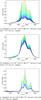 |
Fig. 2 Examples of the destruction of the aliphatic C-H stretching IR absorption feature around 2900 cm-1 during ion irradiation of a-C:H 1 a), a-C:H 2 b), and soot c). The upper (red) line is the initial spectrum, before irradiation. The optical depth decreases (from green to purple lines in the online coloured version) as the fluence rises. The fluence between two spectra is of the order of few 1012 and few 1013 ions cm-2 for the Si7+ and C6+ irradiations, respectively. |
Because in the astrophysical context the cosmic ray stopping powers are mostly electronic, we checked that the same is true in the irradiation experiments and that the ions are not implanted in the samples. We thus need to calculate the samples thicknesses d. When the interference pattern is visible in the IR spectra, the interfringe Δσ is measured and the sample thicknesses d are calculated using the formula d = 1/(2 n Δσ cos(αIR)), with n the refractive index of the sample, and αIR the angle of the IR beam incidence with the normal of the sample (αIR = 45°). When this pattern is not visible, the sample thicknesses are estimated from the continuum absorbance for soot, and from the 3.4 μm absorbance for a-C:H. The values are given in Table 1. These estimated thicknesses show that for most of the samples, the ions are implanted in the substrate, located behind the sample (the projected ranges Rp calculated with SRIM, i.e. the length the ion covers in the target material before stopping, are greater than the samples thicknesses), and the irradiation beam can be considered mono-energetic within the sample (i.e. ΔE/E ≪ 1, with ΔE the ion energy difference between each of the two sample surfaces). However, this is not the case anymore for 400 keV Ar2+ ions in a-C:H, and 200 keV H+ ions in soot, where the ions are implanted in the sample and the nuclear part of the interaction at the track end becomes substantial. Among the experiments performed in Catania, only the projected range of the 200 keV H+ ions in the a-C:H sample is clearly greater than the sample thickness. Therefore, we will not use the results of these ions with Rp/d ≤ 1, which show different behaviours compared to the other irradiation experiments.
We observed no significant modification of the sample thickness (through the interfringe) during irradiation. Therefore, the sputtering that occurs at the sample surface reduces the thickness by only a few percents at most. We do not consider this effect in the following.
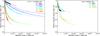 |
Fig. 3 Examples of evolution of the relative integrated optical depth of the aliphatic C-H stretching band with the energy deposited by the ions and the associated fits (recombination model). The deposited energy is calculated from the ion fluence: FE = FI·Se. The a-C:H and soot samples are represented on the left and on the right, respectively. |
3. Results
For all carbonaceous samples, the different irradiations result in an effective2 destruction of the aliphatic C-H component. The optical depths of the sp3 methyl and methylene C-H stretching (around 3.4 μm or 2900 cm-1) and bending modes (6.85 and 7.25 μm, 1460 and 1380 cm-1 respectively) are decreasing during the irradiation (see Fig. 2). The evolution of the optical depth integrated over the aliphatic C-H stretch band (between 2760 and 3140 cm-1) as a function of the deposited energy for different ions/energies is represented in Fig. 3. The evolution of a-C:H 1 (left of Fig. 3) and that of a-C:H 2 (not represented on the figure) for a same ion and energy are very similar (see also Fig. 5).
Other bands appear or disappear with the ion dose as a consequence of the chemical structure modifications induced by ion irradiation. Here, we focus on the dehydrogenation of the material seen through the destruction of aliphatic C-H bonding.
3.1. Determination of the aliphatic C-H destruction parameters by ion irradiation: the recombination model
The integrated optical depth
A = ∫τ dσ of the
sp3 C-H stretching band around 3.4 μm (and bending bands
around 6.9 and 7.3 μm) decreases with the ion fluence, and thus with the
deposited energy (Fig. 3). This evolution can be
fitted by a function of the form 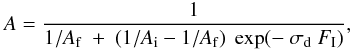 (1)where
FI is the ionic fluence (ion cm-2),
and σd the effective C-H destruction cross section
(cm2 ion-1).
Ai and Af are the initial and
asymptotic value at an infinite dose of the integrated optical depth, respectively. The
value of A is assumed to be proportional to the hydrogen
concentration ρ. The Eq. (1) results then of the equation
(1)where
FI is the ionic fluence (ion cm-2),
and σd the effective C-H destruction cross section
(cm2 ion-1).
Ai and Af are the initial and
asymptotic value at an infinite dose of the integrated optical depth, respectively. The
value of A is assumed to be proportional to the hydrogen
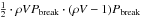
concentration ρ. The Eq. (1) results then of the equation 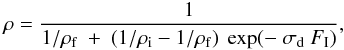 (2)where
ρi and ρf are the initial and
asymptotic value of the hydrogen concentration.
(2)where
ρi and ρf are the initial and
asymptotic value of the hydrogen concentration.
This function, which describes the hydrogen content evolution with ion fluence, results
from a model developed by Adel et al. (1989) and
Marée et al. (1996). This model is based on the
fact that hydrogen leaves the a-C:H films in molecular form (Wild & Koidl 1987; Möller
& Scherzer 1987). Therefore, the hydrogen evolution is based on a second
order kinetic process. In this approach, the recombination of two hydrogen atoms into
molecular hydrogen, which results from the breaking of two C-H bonds by the electronic
energy deposition of a passing ion occurs in the bulk of the irradiated material. The
resulting H2 molecule then rapidly diffuses to the surface and is lost from the
material without further interactions. When a C-H bond is broken, the hydrogen atom
diffuses within a characteristic distance l in the ion track before it is
either trapped by a reactive site in the irradiated material, or is recombined with
another free H atom. This distance defines a recombination volume V,
inside the track of radius r, in which two free hydrogen atoms that are
released by the energy deposition of the same ion can recombine as
a H2 molecule. The probability of breaking a C-H bond with one ion
is Pbreak and the probability of molecular recombination of
two H atoms diffusing in the volume V
is Prec. The number of possible pairs of H atoms that can be
formed by one ion in the volume V is
 . The number of
H atoms lost as H2 molecules per energetic ion in the volume V
is thus
. The number of
H atoms lost as H2 molecules per energetic ion in the volume V
is thus  . The differential
equation that describes the hydrogen depletion of the film with the ion
fluence FI is given by
. The differential
equation that describes the hydrogen depletion of the film with the ion
fluence FI is given by  (3)Equation (2) is the solution for this differential
equation with
(3)Equation (2) is the solution for this differential
equation with  and
ρf = 1/V. When only one hydrogen atom
remains in the recombination volume, then ρV = 1 and the H release via
hydrogen molecular recombination ceases or becomes very improbable. The latter explains
the link between V and the final hydrogen
density ρf. Equation (3) can be written as
and
ρf = 1/V. When only one hydrogen atom
remains in the recombination volume, then ρV = 1 and the H release via
hydrogen molecular recombination ceases or becomes very improbable. The latter explains
the link between V and the final hydrogen
density ρf. Equation (3) can be written as 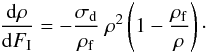 (4)Equation (4) is valid for an irradiation perpendicular to
the sample surface. Otherwise, the angle of incidence should be taken into account in the
section of the ion track. In the irradiation performed in Catania, the ion beam has a
direction of 45° with respect to the sample surface, σd in
previous equations becomes
(4)Equation (4) is valid for an irradiation perpendicular to
the sample surface. Otherwise, the angle of incidence should be taken into account in the
section of the ion track. In the irradiation performed in Catania, the ion beam has a
direction of 45° with respect to the sample surface, σd in
previous equations becomes  .
.
This model can explain the hydrogen depletion induced by ion irradiations in hydrogenated amorphous carbon films. It has been applied for such materials by Adel et al. (1989), Marée et al. (1996), Som et al. (1999), and Baptista et al. (2004), and also to other organic layers (e.g., in Adel et al. 1989; Marée et al. 1996; and Baptista et al. 2004).
We applied to our data fits corresponding to the recombination model, based on Eq. (2), using σd and ρf as adjustable parameters. The best-fit parameters and the associated errors are determined by a χ2 minimisation. The obtained destruction cross section σd, relative final hydrogen content Af/Ai, and corresponding recombination volume V = 1/ρf values for the different experiments are reported in Table 2 (for explanation about the estimation of V, see Sect. 3.3).
Alternatively, the hydrogen concentration decrease can also be fitted assuming a first-order kinetic process (Mennella et al. 2003; Pawlak et al. 1997), with an exponential function and an added constant representing the aliphatic feature residual intensity at high ion fluences. This fit is a simple phenomenological function. In the Appendix, we report the results obtained with this exponential fit and show that Eq. (2), which corresponds to the recombination model, fits our data better.
Results of ion irradiation experiments obtained with the recombination model fits.
3.2. Destruction cross section
We represent in Fig. 4 the different values of σd as a function of the electronic stopping cross section Se for the a-C:H and soot irradiation experiments. For a-C:H, the destruction cross section estimated from the aliphatic C-H bending bands are also plotted. These σd are, as expected, very similar to those determined through the stretching band. The fairly large error bars illustrate the strong dependence of σd on Af with Eq. (1). Effectively, the values of Af are not always well constrained in our data because we lack experimental points at higher fluence. These uncertainties largely depend on the asymptotic behaviour, which requires high ion fluence. The latter is strongly limited by the instantaneous fluxes that should not induce heating of the sample, and by the available time on the ion irradiation facility. The irradiation by 20 MeV helium ions (Se ≈ 0.2 MeV/(mg/cm2)) sets only an upper limit on the destruction cross section because a higher fluence is required. For low Se experiments, this high fluence was difficult to reach without obtaining excessively high ion fluxes.
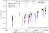 |
Fig. 4 Aliphatic C-H destruction cross section σd obtained with the recombination model as a function of the electronic cross section Se for the different ion/energy irradiation of our a-C:H (filled dots for a-C:H 1, and squares for a-C:H 2) and soot (black asterisks) samples. Cross sections calculated from data of different a-C:H irradiation studies are represented with blue diamonds (Adel et al. 1989; Baptista et al. 2004; Baumann et al. 1987; Fujimoto et al. 1988; González-Hernández et al. 1988; Ingram & McCormick 1988; Marée et al. 1996; Mennella et al. 2003; Pawlak et al. 1997; Prawer et al. 1987; Som et al. 2005, 1999; Zou et al. 1988). See text for details. |
3.2.1. Influence of the material irradiated
a-C:H 1 and a-C:H 2 have similar values of σd. It appears that, although the carbon skeleton and the hydrogen density of these two materials are slightly different, this does not have a strong influence on the destruction cross sections within the explored range. In the case of soots, the σd values are also comparable to those of a-C:H, within the experimental uncertainties (higher for soot than a-C:H). This similarity seems surprising because of the large difference in the H/C ratio, for instance. Soot and a-C:H strongly differ in their carbon skeleton and hydrogen density, the soot being mainly composed of polyaromatic units, poorly organised, and cross-linked by aliphatic bridges. It implies that the aliphatic domains are localised at the edge of the aromatic domains, and that the (aliphatic) hydrogen density is far from being homogeneous within the material. Thus, as long as the recombination volume is smaller than or comparable to the aliphatic domain extent, the hydrogen experiences an environment similar as in a-C:H. It may also indicate that this ionic irradiation does not create efficient reactive sites in the aromatic domains as suggested by the infrared spectra of the irradiated soot. These findings show that only the local environments experienced by the hydrogen atoms, which is identified as the recombination volume, determined the effective destruction cross section.
In Fig. 4 we also plotted the effective destruction cross section (seen through the aliphatic C-H stretch band) of previous a-C:H irradiation experiments (Adel et al. 1989; Baptista et al. 2004; Baumann et al. 1987; Fujimoto et al. 1988; González-Hernández et al. 1988; Ingram & McCormick 1988; Marée et al. 1996; Mennella et al. 2003; Pawlak et al. 1997; Prawer et al. 1987; Som et al. 2005, 1999; Zou et al. 1988). These cross sections were deduced from the available data and using Eq. (1). We did not represent in this figure the experiments where the nuclear cross section plays a role (Sn/Se > 0.5), or where implantation in the sample occurs (d/Rp > 0.9) in order to compare experiments pertaining to the same irradiation conditions. Even if it is difficult to compare results from different experiments, our results and those from previous works are, for most of them, on the same order of magnitude and show the same behaviour with Se. These materials span a wide range of hydrogen atomic concentration, from few to about fifty percents. Therefore, the measured destruction cross sections for aliphatic C-H bonds seem weakly dependent on the irradiated carbonaceous material and may be used as a general characteristic.
Below we will use only our results on a-C:H 1 because they were better explored and thus have lower uncertainties.
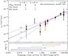 |
Fig. 5 Aliphatic C-H destruction cross section σd as function of the electronic cross section Se for the different ion/energy irradiation of the a-C:H samples. The values corresponding to the C-H stretching modes at 3.4 μm (in black), the CH2 bending mode at 6.85 μm (in red), and the CH3 bending mode at 7.25 μm (in green) are represented for both a-C:H 1 (filled dots) and a-C:H 2 (squares). The best fit and the fits with extreme values of α are plotted (the corresponding values of α are written). The coloured arrows represent the Se range of the few major cosmic ray elements. |
3.2.2. Dependence on the stopping power
The aliphatic C-H destruction cross section seems to vary as a power law
of Se. We fitted the results with:  (5)The
best and extreme fits for our a-C:H results obtained with the recombination model are
shown in Fig. 5. The parameters of this fit for
a-C:H and soot are given in Table 3
(for Se in MeV/(mg/cm2)
and σd in cm2).
(5)The
best and extreme fits for our a-C:H results obtained with the recombination model are
shown in Fig. 5. The parameters of this fit for
a-C:H and soot are given in Table 3
(for Se in MeV/(mg/cm2)
and σd in cm2).
The value of α is not completely determined and lies between 0.5 and 1.7, but the values matching the a-C:H and soot data are between 0.9 and 1.5. In the following, we will use α values of 1.0, 1.2 and 1.4 to show the consequences of different σd behaviours. Mennella et al. (2003) assume a power of 1 (i.e. proportionality between σd and Se), while Baptista et al. (2004) found a power of approximately 2. The model of Marée et al. (1996) not only explains the hydrogen release as a second-order kinetic process, but also explains the dependence of the release rate on the ion stopping power in the material. As they explained, the stopping power appears to be proportional to r2. We saw above that the recombination model predicts values of σd that are also proportional to r2. Thus, in the description given by the model developed by Marée et al. (1996), σd should be proportional to Se (i.e., α = 1). This is compatible with our experimental results.
To compare the stopping cross sections Se explored by our experiments with the Se of cosmic rays, we represented in Figs. 5 and 6 the Se range of a few major cosmic ray elements (coloured arrows in the bottom plots). These ranges are determined for each element, from the Se distribution as a function of the energy (calculated with the SRIM program for each projectile, for H/C ratio and density corresponding to our a-C:H target material) and the cosmic ray distribution of energy. The CR energy from 100 eV/nucleon up to 10 GeV/nucleon are considered because, below and above this energy range, the CR flux becomes either too low and/or the induced destruction is inefficient (cf. Sect. 4.1 and Fig. 8).
3.3. Residual H content and recombination volume
We found that the asymptotic values at infinite fluence of the integrated optical depth of the aliphatic C-H bands is not zero, and thus a fraction of the initial hydrogen content remains in the irradiated material. This residual H content is reached when the C-H bond concentration is low enough so that the free H atoms liberated by an ion are too far from each other to recombine (i.e. the mean distance between H atoms in the material is greater than the radius defined by the recombination volume), and cannot form H2 molecules. The hydrogen is captured by the material and does not escape. In Fig. 6 the parameters Af/Ai obtained from the recombination model fits of a-C:H are represented as a function of the electronic stopping cross section Se. The final hydrogen content decreases when the stopping cross section increases. For the experiments with the lowest stopping cross section (i.e. those with Se < 1 MeV/(mg/cm2)), the value of Af cannot be well determined and only upper limits are obtained.
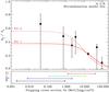 |
Fig. 6 Final relative integrated optical depth Af/Ai of C-H stretching modes, obtained after infinite irradiation as function of the electronic cross section Se for the different irradiation ion/energy of a-C:H 1 samples. Two different fits corresponding to the linear increase of the recombination volume V with Se (Eq. (6)) are plotted: the solid line (fit 1) is the best fit, and the dashed line (fit 2) represents an extreme fit for which the asymptotic Af/Ai are the highest for low Se. The coloured arrows represent the Se range of the few major cosmic ray elements. |
Assuming an initial hydrogen volumic concentration ρi around 5.6 × 10²² H at. cm-3 for a-C:H (estimated from the values of density and H/C ratio given in Sect. 2.1), we obtain ρf from Af/Ai. In the recombination model, the recombination volume V is the inverse of the hydrogen concentration ρf. The estimated values of V are given in Table 2. With the same method, we obtain an estimated mean hydrogen density for soot of 9.0 × 10²⁰ H at. cm-3. However, contrary to a-C:H, the aliphatic hydrogen density is not homogeneous in soot, and is higher in the aliphatic bridges that link the aromatic units. The V estimates for soot given in Table 2 are thus calculated with a local hydrogen density equal to the a-C:H ρi value. The obtained volumes are equivalent to volumes of spheres with angstrom-sized radii.
The diffusion volume values found by Marée et al. (1996) for a-C:H are similar (slightly higher) to ours for equivalent stopping powers. In the a-C:H ion irradiation literature, a residual hydrogen content is also observed at high fluence. These residual content seems compatible with our results. The corresponding diffusion volumes were not estimated because the hydrogen densities of the different samples may not always be homogeneous, and thus ρf cannot be correctly determined. In previous studies, different observations were made concerning the final hydrogen content variation with the stopping power. Adel et al. (1989) report that the final hydrogen content does not depend on the ion beam used in the analysis, and that this final value is approximately 5 at.%. This disagrees with the increase of the recombination volume with the stopping power observed by us and Marée et al. (1996). Baptista et al. (2004) found an opposite correlation, i.e., an increase of the final hydrogen content when the stopping cross section is raised. It should be noted, however, that some of the experiments in this study are driven by an important part of nuclear interactions, thus mixing different mechanisms at work in the interaction with ions.
3.3.1. Dependence on the stopping power
We found that the recombination volume V increases linearly
with Se. The corresponding equation for
a-C:H 1 recombination volume is approximately (V in Å3
and Se in MeV/(mg/cm2)) 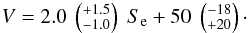 (6)The
best fit of Af/Ai
corresponding to Eq. (6), called
Fit 1 from now, is represented in Fig. 6 by the solid line. The dashed line represents an extreme fit, called
Fit 2, for which the
asymptotic Af/Ai are the
highest for low Se (see Eq. (6)). The fits are determined from the experimental data obtained with
a-C:H 1, but the results obtained with soot samples seem also compatible with both fits.
These best and extreme fits of the residual hydrogen content at high fluence are
compatible with the recombination model. Marée et al.
(1996) explained that the recombination volume should be proportional
to Se if the stopping cross section is proportional
to r2 as explained above.
(6)The
best fit of Af/Ai
corresponding to Eq. (6), called
Fit 1 from now, is represented in Fig. 6 by the solid line. The dashed line represents an extreme fit, called
Fit 2, for which the
asymptotic Af/Ai are the
highest for low Se (see Eq. (6)). The fits are determined from the experimental data obtained with
a-C:H 1, but the results obtained with soot samples seem also compatible with both fits.
These best and extreme fits of the residual hydrogen content at high fluence are
compatible with the recombination model. Marée et al.
(1996) explained that the recombination volume should be proportional
to Se if the stopping cross section is proportional
to r2 as explained above.
The minimum diffusion volumes V corresponding to the maximum Af/Ai value, i.e. the constant in Eq. (6) of 50 Å3 for fit 1 and 32 Å3 for fit 2, is also coherent with the recombination model. These minimum volume values are equivalent to the volume of a sphere with a radius of 2−3 Å, i.e., the approximate distance a between two adjacent hydrogen atoms3. Because the radius of the diffusion volume cannot be lower than a, this explains the presence of a maximum Af/Ai value at low Se. We can also notice that if we assume we can estimate the ion track radius r from the destruction cross section σd by πr2 ~ σd, the transition at Se ~ 1 MeV/(mg/cm2), under which Af/Ai is roughly constant, corresponds to the Se where the diffusion volume is equivalent to a sphere with a radius that equals the ion track radius r.
In the following, if nothing is indicated, the values used for σd and Af/Ai are those determined from the a-C:H data using the recombination model.
4. Astrophysical implications
Using our ion irradiation experiments, we can determine the effective aliphatic C-H destruction cross section σd(Z,EA) and the asymptotic hydrogen content at high fluence ρf(Z,EA) for each ion of atomic number Z and energy per nucleon EA. Below we use these results to infer the evolution of the interstellar aliphatic C-H component exposed to cosmic rays. For this, we take the sum of the entire different cosmic rays ions and energy contributions into account.
4.1. The interstellar cosmic ray flux
We first need to set how many cosmic rays of each ion type and of each energy irradiate
the dust components in the interstellar medium. We call
 the differential flux of
cosmic rays
(particles cm-2 s-1 sr-1 (MeV/nucleon)-1) of
atomic number Z and energy per nucleon EA.
the differential flux of
cosmic rays
(particles cm-2 s-1 sr-1 (MeV/nucleon)-1) of
atomic number Z and energy per nucleon EA.
The Z dependence of this flux is given by the cosmic ray relative abundance of each element A/H(Z) (normalised to hydrogen). Different distributions A/H(Z) found in the literature are represented in Fig. 7 (http://galprop.stanford.edu/, Simpson 1983; Meyer et al. 1998; Fig. 3 of Hörandel 2008, and references therein). Some differences exist between existing distributions in the literature, and we report their resulting effects on ionisation and destruction by cosmic rays in Table 4. We compared the results to the expected ionisation rate by cosmic rays (see Sect. 4.2) and chose to use the CR distribution at 100 MeV/nucleon given by the GALPROP code (reacceleration model, http://galprop.stanford.edu/, Vladimirov et al. 2011). All elements lighter than copper are considered (Z ≤ 29).
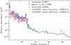 |
Fig. 7 Abundance of elements in cosmic rays as function of their atomic number Z at energies around 0.1−1 GeV/nucleon, normalised to hydrogen (from http://galprop.stanford.edu/, Simpson 1983; Meyer et al. 1998; Fig. 3 of Hörandel 2008, and references therein). |
In the following, we used the CR energy distribution given by Webber & Yushak (1983), providing the protons differential flux
 (particles cm-2 s-1 sr-1 (MeV/nucl)-1) as
 (7)where
EA is the cosmic ray energy per nucleon (in MeV/nucleon),
C = 9.42 × 10⁴ is a normalisation constant, and
E0 = 400 MeV/nucleon is a form parameter that modifies
only the low-energy CR spectra. Because of the solar modulation, the distribution of
low-energy CR is not directly measurable from Earth, and is not fully determined below
10−100 MeV. Padovani et al. (2009) compared two
extreme low-energy CR spectra, with CR fluxes either strongly decreasing or strongly
increasing below 10 MeV. These minimum and maximum distributions are taken from Webber (1998) and Moskalenko et al. (2002), respectively, and are extrapolated below 10 MeV by a
power-law in energy. The adopted maximum distribution appears to be a very high upper
limit. The distribution we adopted is between these two extremes, but more importantly,
Padovani et al. (2009) have calculated that both
these initial distributions obtain roughly constant CR fluxes at low energies (as the one
we adopted) once the CR have traversed and interacted with interstellar matter.
(7)where
EA is the cosmic ray energy per nucleon (in MeV/nucleon),
C = 9.42 × 10⁴ is a normalisation constant, and
E0 = 400 MeV/nucleon is a form parameter that modifies
only the low-energy CR spectra. Because of the solar modulation, the distribution of
low-energy CR is not directly measurable from Earth, and is not fully determined below
10−100 MeV. Padovani et al. (2009) compared two
extreme low-energy CR spectra, with CR fluxes either strongly decreasing or strongly
increasing below 10 MeV. These minimum and maximum distributions are taken from Webber (1998) and Moskalenko et al. (2002), respectively, and are extrapolated below 10 MeV by a
power-law in energy. The adopted maximum distribution appears to be a very high upper
limit. The distribution we adopted is between these two extremes, but more importantly,
Padovani et al. (2009) have calculated that both
these initial distributions obtain roughly constant CR fluxes at low energies (as the one
we adopted) once the CR have traversed and interacted with interstellar matter.
The velocity spectra of different elements are quite similar to each other, hence, as in
Shen et al. (2004), we assume the same normalised
CR energy spectra for each element (when represented as a function of the energy per
nucleon). The GALPROP CR energy distribution data (dotted lines in Fig. 8) show that this assumption is reasonable. The
differential flux of cosmic rays for each element (see Fig. 8) is obtained by combining the differential energy spectra to the cosmic rays
relative abundance 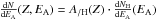 . We
consider the CR energy per nucleon EA between 100 eV and
10 GeV, where the CR flux is not too low and the induced destruction is efficient (out of
this EA range, the electronic stopping power is low and the
destruction cross section is thus also low).
. We
consider the CR energy per nucleon EA between 100 eV and
10 GeV, where the CR flux is not too low and the induced destruction is efficient (out of
this EA range, the electronic stopping power is low and the
destruction cross section is thus also low).
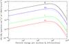 |
Fig. 8 Differential flux dN/dEA distribution with the cosmic ray energy per nucleon EA for some of the cosmic ray elements (hydrogen, helium, oxygen, and iron) (Webber & Yushak 1983; Shen et al. 2004). The dotted lines are the values given by GALPROP (http://galprop.stanford.edu/webrun/, Vladimirov et al. 2011). |
Comparison of the values of η, the ionisation and destruction rates corresponding to the different cosmic ray distribution A/H(Z).
4.2. Ionisation rate
To check if the chosen abundance distribution is coherent, we can link the cosmic ray
fluxes to an astrophysical observable. The interstellar ionisation rate by
cosmic rays Ri,CR (s-1) can be estimated with the
equation 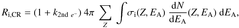 (8)where
the cosmic ray spectra is determined as explained
in the previous section. The cross sections
σi(Z,EA) (cm2/ion)
for the ionisation by energetic ions are estimated from the Bethe equation reported by
Spitzer & Tomasko (1968)
(8)where
the cosmic ray spectra is determined as explained
in the previous section. The cross sections
σi(Z,EA) (cm2/ion)
for the ionisation by energetic ions are estimated from the Bethe equation reported by
Spitzer & Tomasko (1968)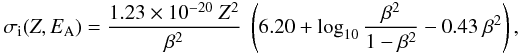 (9)where
β·c is the velocity of the energetic ion.
k2nd e− is the fraction of
the ionisation rate due to the secondary electrons, i.e., the free electrons produced by
the ionisation process and contributing then to ionise other atoms when their energy is
high enough. This factor has a value around
k2nd e− = 0.7 (Cravens & Dalgarno 1978). With the adopted
cosmic ray flux, we found an ionisation rate of
Ri,CR = 2 × 10-17 s-1.
(9)where
β·c is the velocity of the energetic ion.
k2nd e− is the fraction of
the ionisation rate due to the secondary electrons, i.e., the free electrons produced by
the ionisation process and contributing then to ionise other atoms when their energy is
high enough. This factor has a value around
k2nd e− = 0.7 (Cravens & Dalgarno 1978). With the adopted
cosmic ray flux, we found an ionisation rate of
Ri,CR = 2 × 10-17 s-1.
Most of the  observations
in the diffuse interstellar medium give values of cosmic-ray ionisation rate between 2 ×
10-17 s-1 and 4 × 10-16 s-1 (Webber 1998; Dalgarno
2006; Indriolo et al. 2007, 2009). However, a value of 1.2 ×
10-15 s-1 is inferred by McCall
et al. (2003). The ionisation rate calculated from the different CR abundance
distributions of Fig. 7 are all equal to
a few 10-17 s-1. Moreover, the contribution of the CR heavy ions
(other than hydrogen) in the ionisation rate is often considered to be a factor about
equal to 1.8 of the contribution of hydrogen (Spitzer
& Tomasko 1968; Shen et al. 2004).
This factor can be calculated as the sum
η = ∑ A/H(Z) Z2
(cf. Eqs. (8) and (9)). With the adopted GALPROP distribution, we
found η = 1.8, which agrees reasonably well. Table 4 shows a comparison of η
and Ri,CR found with the different
CR distributions A/H(Z).
observations
in the diffuse interstellar medium give values of cosmic-ray ionisation rate between 2 ×
10-17 s-1 and 4 × 10-16 s-1 (Webber 1998; Dalgarno
2006; Indriolo et al. 2007, 2009). However, a value of 1.2 ×
10-15 s-1 is inferred by McCall
et al. (2003). The ionisation rate calculated from the different CR abundance
distributions of Fig. 7 are all equal to
a few 10-17 s-1. Moreover, the contribution of the CR heavy ions
(other than hydrogen) in the ionisation rate is often considered to be a factor about
equal to 1.8 of the contribution of hydrogen (Spitzer
& Tomasko 1968; Shen et al. 2004).
This factor can be calculated as the sum
η = ∑ A/H(Z) Z2
(cf. Eqs. (8) and (9)). With the adopted GALPROP distribution, we
found η = 1.8, which agrees reasonably well. Table 4 shows a comparison of η
and Ri,CR found with the different
CR distributions A/H(Z).
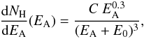
4.3. Destruction rate
The destruction rate Rd,CR (s-1) of the
interstellar aliphatic C-H component by cosmic rays can be calculated as defined by Mennella et al. (2003). 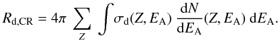 (10)Using
the SRIM code to calculate the expected stopping cross
section Se as a function of the atomic
number Z and of the energy per nucleon EA,
and the relation established in the previous section
linking σd(Z,EA)
to Se(Z,EA), we
determined the aliphatic C-H destruction cross section for each ion and energy of
cosmic rays. By applying Eq. (10), we find
an interstellar aliphatic C-H destruction rate by cosmic rays
Rd,CR = 3.1 × 10⁻¹⁷ s-1
(corresponding to α = 1.4), Rd,CR = 6.1 ×
10-17 s-1 (corresponding to α = 1.2) and
Rd,CR = 1.6 × 10⁻¹⁶ s-1
(α = 1.0). These values are one order of magnitude lower than the value
found by Mennella et al. (2003).
Rd,CR found with the different
CR distribution A/H(Z) are compared in
Table 4. This destruction rate as calculated by
Mennella et al. (2003) does not consider the
value of the residual C-H aliphatic content at high fluence.
(10)Using
the SRIM code to calculate the expected stopping cross
section Se as a function of the atomic
number Z and of the energy per nucleon EA,
and the relation established in the previous section
linking σd(Z,EA)
to Se(Z,EA), we
determined the aliphatic C-H destruction cross section for each ion and energy of
cosmic rays. By applying Eq. (10), we find
an interstellar aliphatic C-H destruction rate by cosmic rays
Rd,CR = 3.1 × 10⁻¹⁷ s-1
(corresponding to α = 1.4), Rd,CR = 6.1 ×
10-17 s-1 (corresponding to α = 1.2) and
Rd,CR = 1.6 × 10⁻¹⁶ s-1
(α = 1.0). These values are one order of magnitude lower than the value
found by Mennella et al. (2003).
Rd,CR found with the different
CR distribution A/H(Z) are compared in
Table 4. This destruction rate as calculated by
Mennella et al. (2003) does not consider the
value of the residual C-H aliphatic content at high fluence.
4.4. Comprehensive description of the aliphatic C-H evolution under interstellar cosmic ray irradiation
We now describe in more detail the evolution of the interstellar aliphatic C-H component
under cosmic ray irradiation, represented by the
variable ρ(t). 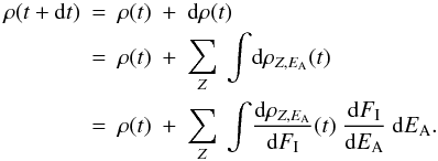 The
units of
The
units of  are ions cm-2 (MeV/nucl)-1 and this variable can be expressed as a
function of the cosmic ray differential flux:
are ions cm-2 (MeV/nucl)-1 and this variable can be expressed as a
function of the cosmic ray differential flux: 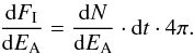 The
equation describing the evolution of the aliphatic C-H concentration in interstellar
materials becomes
The
equation describing the evolution of the aliphatic C-H concentration in interstellar
materials becomes 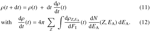 The
value
The
value  represents the destruction
of the interstellar C-H aliphatic component at instant t by the whole
distribution of cosmic ray ions and energies. For the recombination model, we can write
represents the destruction
of the interstellar C-H aliphatic component at instant t by the whole
distribution of cosmic ray ions and energies. For the recombination model, we can write
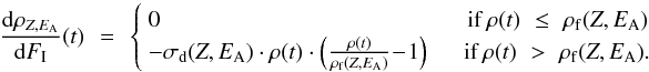 When
ρ(t) is beyond the asymptotic value
ρf(Z,EA), the
cosmic rays of atomic number Z and of energy per
nucleon EA do not participate anymore in the destruction.
As a result,
When
ρ(t) is beyond the asymptotic value
ρf(Z,EA), the
cosmic rays of atomic number Z and of energy per
nucleon EA do not participate anymore in the destruction.
As a result,  for
ρ(t) ≤ ρf(Z,EA).
The σd(Z,EA) and
ρf(Z,EA) values
are calculated for each ion and energy from the behaviour of irradiated a-C:H samples with
the stopping cross section Se (Figs. 5 and 6, respectively). The
temporal evolution of the C-H aliphatic component of the interstellar matter under cosmic
ray is represented in Fig. 9. Note that the
destruction rate Rd,CR defined above corresponds to the value
of
for
ρ(t) ≤ ρf(Z,EA).
The σd(Z,EA) and
ρf(Z,EA) values
are calculated for each ion and energy from the behaviour of irradiated a-C:H samples with
the stopping cross section Se (Figs. 5 and 6, respectively). The
temporal evolution of the C-H aliphatic component of the interstellar matter under cosmic
ray is represented in Fig. 9. Note that the
destruction rate Rd,CR defined above corresponds to the value
of  if ρ follows an exponential decrease with
ρf = 0. This exponential decrease
ρ/ρi = exp(−Rd,CR·t)
(only the values of
σd(Z,EA) are
considered in the previous equations, and
ρf(Z,EA) = 0)
is also reported in Fig. 9 (black line) for sake of
comparison. The relative destruction of the C-H aliphatic component %d
corresponding to a typical cloud time scale t = 3 ×
107 years (McKee 1989; Draine 1990; Jones
et al. 1994) are given in Table 5 for the
different adopted fits.
if ρ follows an exponential decrease with
ρf = 0. This exponential decrease
ρ/ρi = exp(−Rd,CR·t)
(only the values of
σd(Z,EA) are
considered in the previous equations, and
ρf(Z,EA) = 0)
is also reported in Fig. 9 (black line) for sake of
comparison. The relative destruction of the C-H aliphatic component %d
corresponding to a typical cloud time scale t = 3 ×
107 years (McKee 1989; Draine 1990; Jones
et al. 1994) are given in Table 5 for the
different adopted fits.
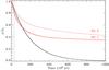 |
Fig. 9 Evolution of the C-H aliphatic component of the interstellar matter under cosmic ray irradiation. The values of σd were determined from a-C:H 1 data with α = 1.0 (see Fig. 5). The black curve corresponds to an exponential decrease without residual hydrogen content taking into account (ρ/ρi = exp(−Rd,CR·t)). The red solid (fit 1) and dashed (fit 2) curves are obtained when the asymptotic values ρf/ρi ≠ 0 are considered. Values of ρf/ρi are determined from a-C:H 1 data and two different fits (see Fig. 6 and text for details). The dotted vertical line corresponds to a typical cloud time scale t = 3 × 10⁷ yr. (McKee 1989; Draine 1990; Jones et al. 1994). |
Percentage of destruction %d at a typical cloud time scale t = 3 × 10⁷ yrs for the different fits adopted concerning σd and Af/Ai.
4.5. Heavy ions contribution
In the destruction rate calculation (i.e., exponential decrease not taking into account the residual hydrogen content), the cosmic ray heavy ions contribution to ionisation and destruction are constant in time. These contributions are summarised in Table 6.
Taking into account the residual hydrogen content after long irradiation, the destruction caused by the contribution of ions heavier than hydrogen and helium increases with time (see Fig. 10). The contribution of abundant light CR elements becomes insignificant when the corresponding Af/Ai is reached, and then, only heavier elements pursue the destruction. In Fig. 10 we can see that for α = 1.0, this transition where heavy elements begin to dominate the destruction occurs after irradiation of few hundreds of million years. This corresponds to a time greater than or of the same order as an interstellar cloud lifetime. When α = 1.4, heavy elements contribution is dominant from the beginning of the CR exposure. This is the case when α ≥ 1.3 for the fit 1, and when α ≥ 1.2 for the fit 2.
In every case, the contribution of heavy elements, and particularly of iron ions, is important. Although the Fe ions are less abundant by four orders of magnitude than hydrogen in cosmic rays, they represent a contribution to the aliphatic C-H destruction by cosmic rays between 5% and 40% (with t ≤ 108 years).
Contribution of each major CR element in the abundance, ionisation, and destruction when Af/Ai = 0 is considered.
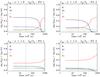 |
Fig. 10 Variation of |

4.6. Evolution of the 3.4 μm feature between diffuse and dense phases of interstellar medium
In this paragraph we discuss the contribution of cosmic rays in the destruction of the interstellar aliphatic C-H component. This will be compared to the interstellar destruction by UV photons, and to the formation by H atoms exposure. These processes are confronted in the different environments of the ISM. The examination of the diffuse and dense interstellar regions will show the need to consider the intermediate regions, too. This discussion is summarised in Table 7.
As shown in Fig. 9, the characteristic destruction time td,CR of the interstellar 3.4 μm absorption feature by cosmic rays is of few 108 years, a time greater than the typical lifetime of interstellar clouds tcloud = 3 × 10⁷ yr. Moreover, by considering in an astrophysical model the asymptotic values at infinite fluence Af ≠ 0, we found that, even at a longer time, the destruction by cosmic rays is not total (after 1 × 10⁹ yr, the destruction did not go further than 65%). These results are valid for both the diffuse and dense interstellar medium because the CR flux is the same in both regions. This clearly confirms that cosmic ray irradiation cannot be the only process responsible for the 3.4 μm absorption feature disappearance in the dense interstellar medium.
Indeed, when they are present, the UV photons dominate the destruction. The destruction of C-H bonds by UV irradiation has been studied by Muñoz Caro et al. (2001) in hydrocarbon molecules and by Mennella et al. (2001) in hydrocarbon grains. They found a destruction cross section σd,UV = 1.0 × 10⁻¹⁹ cm2/photon. They also found that this dehydrogenation process is still efficient with a thin ice layer, without apparent modification of σd,UV.
Synthetic table giving the characteristic times of destruction and formation processes of the aliphatic hydrogenated carbon component in the different phases of the interstellar medium.
4.6.1. Diffuse interstellar medium
In diffuse clouds, an interstellar radiation flux of about 8 ×
107 photons cm-2 s-1 (Mathis et al. 1983), combined with σd,UV found by
Mennella et al. (2001), gives a characteristic
destruction time by exposure to UV radiation  ×
103 years, a time much shorter than for the destruction by cosmic rays. The
destruction of the interstellar 3.4 μm feature in diffuse medium is
thus most probably caused by the UV field in these regions rather than by
CR interactions. The ubiquitous presence of the aliphatic 3.4 μm
feature in the diffuse interstellar medium requires an efficient formation mechanism in
these regions to balance the destruction by UV and cosmic rays, possibly by exposure to
atomic hydrogen (Mennella et al. 1999, 2002; Mennella
2006). Mennella (2006) found a cross
section of C-H bond formation by exposure to H atoms
σf,H = 1.7 × 10⁻¹⁸ cm2/H atom for a
temperature of 100 K of H atoms in diffuse clouds (this cross section decreases when the
temperature drops). A flux of 8 ×
106 H atoms cm-2 s-1 in diffuse clouds (Sorrell 1990) corresponds to a characteristic
formation time in diffuse clouds
×
103 years, a time much shorter than for the destruction by cosmic rays. The
destruction of the interstellar 3.4 μm feature in diffuse medium is
thus most probably caused by the UV field in these regions rather than by
CR interactions. The ubiquitous presence of the aliphatic 3.4 μm
feature in the diffuse interstellar medium requires an efficient formation mechanism in
these regions to balance the destruction by UV and cosmic rays, possibly by exposure to
atomic hydrogen (Mennella et al. 1999, 2002; Mennella
2006). Mennella (2006) found a cross
section of C-H bond formation by exposure to H atoms
σf,H = 1.7 × 10⁻¹⁸ cm2/H atom for a
temperature of 100 K of H atoms in diffuse clouds (this cross section decreases when the
temperature drops). A flux of 8 ×
106 H atoms cm-2 s-1 in diffuse clouds (Sorrell 1990) corresponds to a characteristic
formation time in diffuse clouds  ×
103 yr. Thus, in diffuse clouds, the evolution of the interstellar
3.4 μm absorption feature is governed by its formation due to
exposure to H atoms, and its destruction mainly due to UV irradiation. The resulting
balance between formation and destruction is in favour of the formation in these diffuse
regions.
×
103 yr. Thus, in diffuse clouds, the evolution of the interstellar
3.4 μm absorption feature is governed by its formation due to
exposure to H atoms, and its destruction mainly due to UV irradiation. The resulting
balance between formation and destruction is in favour of the formation in these diffuse
regions.
4.6.2. Dense interstellar medium
In dense molecular clouds, the 3.4 μm feature with a profile associated with the methyl and methylene substructures, which is characteristic of diffuse ISM hydrocarbons, is not observed. This 3.4 μm band with substructures must not be confused with the featureless broad band at 3.47 μm that is seen in dense clouds, and whose the optical depth is correlated with the water ice one. Observations with high signal-to-noise ratio show that the upper limit on the 3.4 μm optical depth in dense clouds is low. It suggests that the carriers of this band are absent from these regions, or at most present in very small quantities.
In dense clouds, the 3.4 μm feature formation process is impeded by several factors: (1) most of the hydrogen is in molecular form, the flux of H atoms is reduced by two orders of magnitude compared to diffuse ISM. (2) Dust grains in dense regions are expected to be covered by an ice layer that prevents the hydrogenation of the material by H atoms. (3) The formation cross section for a temperature of 10 K of H atoms in dense clouds is expected to be three orders of magnitude lower than for the H atom temperature in diffuse clouds (Mennella 2006). Therefore, the methyl and methylene aliphatic C-H formation process probably remains ineffective in dense regions, while the destruction by cosmic rays still proceeds (the presence of an ice layer does not seem to affect the destruction cross section by CR as shown by Mennella et al. (2003)).
Recently, another hypothesis concerning the exposure to H atoms in dense clouds has been proposed in Mennella (2008) and Mennella (2010). He exposed carbon particles covered with a water ice layer to H atoms. These experiments, under simulated dense ISM conditions, result in no observed formation of aliphatic C-H bonds in the CH2 and CH3 functional groups (i.e., those responsible for the 3.4 μm absorption feature observed in diffuse ISM), but a large absorption band around 3.47 μm appears in the IR spectrum. He assigned this band to the C-H stretching vibration of tertiary sp3 carbon atoms and proposed that the interstellar aliphatic 3.4 μm band observed in diffuse regions becomes the 3.47 μm in dense clouds after interstellar processing.
Although the 3.4 μm feature destruction prevails in dense interstellar medium, this work shows that cosmic rays alone cannot account for its apparent disappearance within the cloud lifetime. The galactic UV field cannot penetrate the dense clouds and thus cannot account for an additional destruction. Interestingly, the interaction of galactic cosmic rays with the interstellar medium creates an internal UV field owing to CR-induced H2 fluorescence (Prasad & Tarafdar 1983). The corresponding flux is estimated to be of about 103−104 photons cm-2 s-1. The related destruction time is ~107−108 years. Above a certain AV, when ices appear, a majority of these UV photons is probably absorbed by the ice layers and does not affect the aliphatic C-H component. In dense clouds, the destruction time by internal UV field is thus longer than ~107−108 years, except when the ice does not cover the dust grains yet, i.e. for AV ≲ 3 (Whittet et al. 1988; Smith et al. 1993; Murakawa et al. 2000). In this case, the effect of UV induced by CR can be 10 times greater than that of CR themselves. This internal UV field is thus a non negligible indirect destruction process induced by cosmic rays, but still does not seem to be enough to account for the entire (or almost entire) 3.4 μm destruction.
4.6.3. Interface between diffuse and dense regions
It seems that the disappearance of the 3.4 μm absorption band does not occur in either dense molecular clouds or in the diffuse ISM, but rather in intermediate regions, such as translucent clouds and photon dominated regions. In these interstellar phases, the recombination of H atoms into molecular hydrogen occurs and the atomic hydrogen quantity begins to decrease for visual extinction AV ~ 10-4−10-3 (Le Petit et al. 2006). The lower abundance of H atoms makes the “rehydrogenation” become less efficient in these regions, with a characteristic formation time that is probably much longer. The external UV field decreases as exp(−kAV). As shown in Table 7, between AV ~ 10-3 and AV of a few magnitude units, the atomic hydrogen quantity is lower than in diffuse ISM, and the UV flux is still intense to dehydrogenate the 3.4 μm feature carriers. In these regions, the destruction of this component should be efficient enough to make the 3.4 μm feature disappear in dense regions. Unfortunately, in these regions at the interface between diffuse and dense ISM, observations would not easily provide additional constraints on this scenario because an eventual 3.4 μm absorption feature would be masked by other strong emission features. Mennella et al. (2001, 2003) have proposed the material circulation in the dense cloud (only 1% of the cloud lifetime in the cloud edges is necessary to process the dust by external UV field) or the penetration of the external UV field in filamentary structures as alternative possible explanations.
5. Conclusion
We have performed experiments of irradiation by energetic ions of carbonaceous interstellar analogues (a-C:H and soot). The progressive dehydrogenation of the materials induced by the irradiations was measured through the monitoring of the aliphatic C-H vibration bands in the near- and mid-infrared. The topic has been previously investigated by Mennella et al. (2003) using low-energy ion irradiation (30 keV He ions) coupled to an extrapolation. In this study, we went beyond by addressing in particular the following points: (i) different elements and energies were used, allowing us to explore a wide range of electronic stopping cross sections, comparable to those of cosmic rays. (ii) The recombination model, which explains the observed dehydrogenation through the molecular recombination of two liberated hydrogen atoms in the bulk of the irradiated material, was used to extract the characteristic C-H destruction parameters (destruction cross section and residual hydrogen content at high fluence). (iii) The behaviour of these parameters with the electronic stopping cross section was deduced from our experiments. (iv) In particular, the observed residual hydrogen content at infinite irradiation dose, in agreement with the recombination model, were taken into account in our analysis, and we found that the corresponding recombination volumes are related to the electronic stopping cross section by a linear expression. These results were used to infer the effect of cosmic rays on the interstellar aliphatic C-H component. (v) Although a-C:H and soot samples have a different structure and hydrogen content, no significant difference in the destruction parameters was observed, suggesting that a slightly different material than our a-C:H samples as carrier for the 3.4 μm band would not modify these results.
We showed that the destruction of aliphatic C-H bonds by cosmic rays occurs in characteristic times of few 108 years and is not complete even at longer time scales. The contribution of heavy elements (of the iron element in particular) to this destruction is important. We compared these results to the processing by UV photons and H atoms in the different interstellar phases. As shown by Mennella et al. (2003), in the diffuse ISM the destruction by cosmic rays is negligible compared to the destruction by UV radiation. The hydrogenation by H atoms exceeds the dehydrogenation (mainly by UV photons) in these regions, which explains the 3.4 μm band observations. In dense clouds, the formation by H atoms exposure is ineffective, the galactic UV field cannot penetrate, and only destruction by cosmic rays (directly and indirectly through the created internal UV field) can process the dust grains. However, the diffuse ISM 3.4 μm band is not observed in dense regions and the cosmic rays only cannot account for this disappearance. We conclude that the destruction (or modification) of the interstellar aliphatic C-H component most probably occurs in intermediate regions, where UV and cosmic ray destruction dominate the formation by hydrogen atoms.
The irradiation of interstellar dust by cosmic rays is not the most efficient process to dehydrogenate, but cosmic rays are almost never shielded, and this processing is thus present in all interstellar regions. To fully understand the evolution of interstellar dust under this energetic processing, some work still needs to be done. In the experiments presented here, we took care to irradiate our samples with low fluxes to avoid heating the materials. Even if the temperature effect should not be major, it would be interesting to perform these experiments in conditions closer to those of the interstellar medium, i.e., at low temperature (the hydrogen mobility decrease could influence the value of the destruction parameters). The destruction effect of secondary electrons (created by the cosmic rays) was not taken into account in this work. These low-energy electrons (~30 eV) have a short projected range. In dense regions, they are stopped in the ice mantles, and only alter the surface of dust grains in diffuse regions. Even if only a small fraction of the dust in diffuse medium is affected, it would be interesting to explore the effect of these secondary electrons. The recombination model we used to describe the dehydrogenation process is valid when the interaction of the ion can be considered to be continuous along the track in the material. This could not be the case for ions with low stopping power. More irradiation experiments with high fluence of these ions would allow to check if a different regime occurs at low Se. Moreover, we only discuss the destruction of the aliphatic C-H bonds, but we saw the variation of other IR bands under ion irradiation. Another step in the study will explore these variations, which should give us information about the structural modifications induced by ion irradiation.
The galactic CR flux is of the order of 20 ions cm s.
As explained in Sect. 3.1, C-H bonds are broken by impinging ions, but some of the free H atoms form new bonds in the material.
Å with our estimate at. cm for a-C:H.
Acknowledgments
We would like to thank Dominique Deboffle, Philippe Duret, Thierry Redon and Raymond Vasquez for their help with the experimental developments, Vincent Guerrini for making dedicated vacuum vessels, and Pierre de Marcellus for allowing us to borrow the IR spectrometer. Finally, we aknowledge G. Muñoz Caro for helpful comments on this paper. This work was in part supported by the ANR COSMISME project, grant ANR-2010-BLAN-0502 of the French Agence Nationale de la Recherche, by the French INSU-CNRS national program “Physique et Chimie du Milieu Interstellaire” (PCMI), and by the Paris Sud University “Programme Pluri-Formation” (PPF). This research has made use of NASA’s Astrophysics Data System.
References
- Adamson, A. J., Whittet, D. C. B., & Duley, W. W. 1990, MNRAS, 243, 400 [NASA ADS] [Google Scholar]
- Adel, M. E., Amir, O., Kalish, R., & Feldman, L. C. 1989, J. Appl. Phys., 66, 3248 [NASA ADS] [CrossRef] [Google Scholar]
- Allamandola, L. J., Sandford, S. A., Tielens, A. G. G. M., & Herbst, T. M. 1993, Science, 260, 64 [NASA ADS] [CrossRef] [PubMed] [Google Scholar]
- Baptista, D. L., Garcia, I. T. S., & Zawislak, F. C. 2004, Nucl. Instrum. Methods Phys. Res. B, 219, 846 [Google Scholar]
- Baumann, H., Rupp, T., Bethge, K., Koidl, P., & Wild, C. 1987, Eur. Mater. Res. Soc. Conf. Proc., 17, 343 [Google Scholar]
- Bond, T. C., & Bergstrom, R. W. 2006, Aerosol Science and Technology, 40, 27 [CrossRef] [Google Scholar]
- Bottinelli, S., Adwin Boogert, A. C., Bouwman, J., et al. 2010, ApJ, 718, 1100 [NASA ADS] [CrossRef] [Google Scholar]
- Brooke, T. Y., Sellgren, K., & Geballe, T. R. 1999, ApJ, 517, 883 [NASA ADS] [CrossRef] [Google Scholar]
- Brunetto, R., Baratta, G. A., & Strazzulla, G. 2004, J. Appl. Phys., 96, 380 [NASA ADS] [CrossRef] [Google Scholar]
- Brunetto, R., Pino, T., Dartois, E., et al. 2009, Icarus, 200, 323 [NASA ADS] [CrossRef] [Google Scholar]
- Chiar, J. E., Adamson, A. J., & Whittet, D. C. B. 1996, ApJ, 472, 665 [NASA ADS] [CrossRef] [Google Scholar]
- Chiar, J. E., Tielens, A. G. G. M., Whittet, D. C. B., et al. 2000, ApJ, 537, 749 [NASA ADS] [CrossRef] [Google Scholar]
- Cravens, T. E., & Dalgarno, A. 1978, ApJ, 219, 750 [NASA ADS] [CrossRef] [Google Scholar]
- Dalgarno, A. 2006, Proceedings of the National Academy of Science, 103, 12269 [NASA ADS] [CrossRef] [Google Scholar]
- Dartois, E., & d’Hendecourt, L. 2001, A&A, 365, 144 [NASA ADS] [CrossRef] [EDP Sciences] [Google Scholar]
- Dartois, E., d’Hendecourt, L., Thi, W., Pontoppidan, K. M., & van Dishoeck, E. F. 2002, A&A, 394, 1057 [NASA ADS] [CrossRef] [EDP Sciences] [Google Scholar]
- Dartois, E., Muñoz Caro, G. M., Deboffle, D., Montagnac, G., & D’Hendecourt, L. 2005, A&A, 432, 895 [NASA ADS] [CrossRef] [EDP Sciences] [Google Scholar]
- Dartois, E., Geballe, T. R., Pino, T., et al. 2007, A&A, 463, 635 [NASA ADS] [CrossRef] [EDP Sciences] [Google Scholar]
- Draine, B. T. 1990, in The Evolution of the Interstellar Medium, ed. L. Blitz, ASP Conf. Ser., 12, 193 [Google Scholar]
- Elmegreen, B. G. 2007, ApJ, 668, 1064 [NASA ADS] [CrossRef] [Google Scholar]
- Fujimoto, F., Tanaka, M., Iwata, Y., et al. 1988, Nucl. Instrum. Methods Phys. Res. B, 33, 792 [Google Scholar]
- Glover, S. C. O., & Mac Low, M. 2007, ApJ, 659, 1317 [NASA ADS] [CrossRef] [Google Scholar]
- Godard, M., & Dartois, E. 2010, A&A, 519, A39 [NASA ADS] [CrossRef] [EDP Sciences] [Google Scholar]
- Goldsmith, P. F., Li, D., & Krčo, M. 2007, ApJ, 654, 273 [NASA ADS] [CrossRef] [Google Scholar]
- González-Hernández, J., Asomoza, R., Reyes-Mena, A., et al. 1988, J. Vacuum Sci. Techn., 6, 1798 [NASA ADS] [CrossRef] [Google Scholar]
- Hörandel, J. R. 2008, Adv. Space Res., 41, 442 [NASA ADS] [CrossRef] [Google Scholar]
- Indriolo, N., Geballe, T. R., Oka, T., & McCall, B. J. 2007, ApJ, 671, 1736 [NASA ADS] [CrossRef] [Google Scholar]
- Indriolo, N., Fields, B. D., & McCall, B. J. 2009, ApJ, 694, 257 [NASA ADS] [CrossRef] [Google Scholar]
- Ingram, D. C., & McCormick, A. W. 1988, Nucl. Instrum. Methods Phys. Res. B, 34, 68 [Google Scholar]
- Jones, A. P., Tielens, A. G. G. M., Hollenbach, D. J., & McKee, C. F. 1994, ApJ, 433, 797 [NASA ADS] [CrossRef] [Google Scholar]
- Le Petit, F., Nehmé, C., Le Bourlot, J., & Roueff, E. 2006, ApJS, 164, 506 [NASA ADS] [CrossRef] [EDP Sciences] [Google Scholar]
- Marée, C., Vredenberg, A., & Habraken, F. 1996, Mater. Chem. Phys., 46, 198 [Google Scholar]
- Mathis, J. S., Mezger, P. G., & Panagia, N. 1983, A&A, 128, 212 [NASA ADS] [Google Scholar]
- McCall, B. J., Huneycutt, A. J., Saykally, R. J., et al. 2003, Nature, 422, 500 [NASA ADS] [CrossRef] [PubMed] [Google Scholar]
- McKee, C. 1989, in Interstellar Dust, ed. L. J. Allamandola, & A. G. G. M. Tielens, IAU Symp., 135, 431 [Google Scholar]
- Mennella, V. 2006, ApJ, 647, L49 [NASA ADS] [CrossRef] [Google Scholar]
- Mennella, V. 2008, ApJ, 682, L101 [NASA ADS] [CrossRef] [Google Scholar]
- Mennella, V. 2010, ApJ, 718, 867 [NASA ADS] [CrossRef] [Google Scholar]
- Mennella, V., Brucato, J. R., Colangeli, L., & Palumbo, P. 1999, ApJ, 524, L71 [NASA ADS] [CrossRef] [Google Scholar]
- Mennella, V., Muñoz Caro, G. M., Ruiterkamp, R., et al. 2001, A&A, 367, 355 [NASA ADS] [CrossRef] [EDP Sciences] [Google Scholar]
- Mennella, V., Brucato, J. R., Colangeli, L., & Palumbo, P. 2002, ApJ, 569, 531 [CrossRef] [Google Scholar]
- Mennella, V., Baratta, G. A., Esposito, A., Ferini, G., & Pendleton, Y. J. 2003, ApJ, 587, 727 [NASA ADS] [CrossRef] [EDP Sciences] [Google Scholar]
- Meyer, J., Drury, L. O., & Ellison, D. C. 1998, Space Sci. Rev., 86, 179 [NASA ADS] [CrossRef] [Google Scholar]
- Möller, W., & Scherzer, B. M. U. 1987, Appl. Phys. Lett., 50, 1870 [NASA ADS] [CrossRef] [Google Scholar]
- Moskalenko, I. V., Strong, A. W., Ormes, J. F., & Potgieter, M. S. 2002, ApJ, 565, 280 [Google Scholar]
- Mouschovias, T. C., Tassis, K., & Kunz, M. W. 2006, ApJ, 646, 1043 [NASA ADS] [CrossRef] [Google Scholar]
- Muñoz Caro, G. M., Ruiterkamp, R., Schutte, W. A., Greenberg, J. M., & Mennella, V. 2001, A&A, 367, 347 [NASA ADS] [CrossRef] [EDP Sciences] [Google Scholar]
- Murakawa, K., Tamura, M., & Nagata, T. 2000, ApJS, 128, 603 [NASA ADS] [CrossRef] [Google Scholar]
- Padovani, M., Galli, D., & Glassgold, A. E. 2009, A&A, 501, 619 [NASA ADS] [CrossRef] [EDP Sciences] [Google Scholar]
- Pawlak, F., Paumier, E., Toulemonde, M., et al. 1997, Nucl. Instrum. Methods Phys. Res. B, 131, 135 [Google Scholar]
- Pendleton, Y. J., & Allamandola, L. J. 2002, ApJS, 138, 75 [NASA ADS] [CrossRef] [Google Scholar]
- Pendleton, Y. J., Sandford, S. A., Allamandola, L. J., Tielens, A. G. G. M., & Sellgren, K. 1994, ApJ, 437, 683 [NASA ADS] [CrossRef] [Google Scholar]
- Pino, T., Dartois, E., Cao, A.-T., et al. 2008, A&A, 490, 665 [CrossRef] [EDP Sciences] [Google Scholar]
- Prasad, S. S., & Tarafdar, S. P. 1983, ApJ, 267, 603 [NASA ADS] [CrossRef] [Google Scholar]
- Prawer, S., Kalish, R., Adel, M., & Richter, V. 1987, J. Appl. Phys., 61, 4492 [NASA ADS] [CrossRef] [Google Scholar]
- Sandford, S. A., Allamandola, L. J., Tielens, A. G. G. M., et al. 1991, ApJ, 371, 607 [NASA ADS] [CrossRef] [PubMed] [Google Scholar]
- Shen, C. J., Greenberg, J. M., Schutte, W. A., & van Dishoeck, E. F. 2004, A&A, 415, 203 [NASA ADS] [CrossRef] [EDP Sciences] [Google Scholar]
- Simpson, J. A. 1983, Ann. Rev. Nucl. Part. Sci., 33, 323 [Google Scholar]
- Smith, R. G., Sellgren, K., & Brooke, T. Y. 1993, MNRAS, 263, 749 [NASA ADS] [CrossRef] [Google Scholar]
- Som, T., Kumar, S., & Kulkarni, V. N. 1999, Nucl. Instrum. Methods Phys. Res. B, 156, 212 [Google Scholar]
- Som, T., Malhotra, M., Kulkarni, V. N., & Kumar, S. 2005, Physica B Condensed Matter, 355, 72 [NASA ADS] [CrossRef] [Google Scholar]
- Sorrell, W. H. 1990, MNRAS, 243, 570 [NASA ADS] [Google Scholar]
- Spitzer, Jr., L., & Tomasko, M. G. 1968, ApJ, 152, 971 [NASA ADS] [CrossRef] [Google Scholar]
- Spoon, H. W. W., Armus, L., Cami, J., et al. 2004, ApJS, 154, 184 [NASA ADS] [CrossRef] [Google Scholar]
- Strazzulla, G., Baratta, G. A., Leto, G., Palumbo, M. E., & Spinella, F. 2001, in Exo-/Astro-Biology, ed. P. Ehrenfreund, O. Angerer, & B. Battrick, ESA SP, 496, 129 [Google Scholar]
- Tassis, K., & Mouschovias, T. C. 2004, ApJ, 616, 283 [NASA ADS] [CrossRef] [Google Scholar]
- Vladimirov, A., Digel, S., Jóhannesson, G., et al. 2011, Comput. Phys. Commun., 182, 1156 [NASA ADS] [CrossRef] [Google Scholar]
- Webber, W. R. 1998, ApJ, 506, 329 [Google Scholar]
- Webber, W. R., & Yushak, S. M. 1983, ApJ, 275, 391 [Google Scholar]
- Whittet, D. C. B., Bode, M. F., Longmore, A. J., et al. 1988, MNRAS, 233, 321 [NASA ADS] [CrossRef] [Google Scholar]
- Whittet, D. C. B., Boogert, A. C. A., Gerakines, P. A., et al. 1997, ApJ, 490, 729 [NASA ADS] [CrossRef] [Google Scholar]
- Wickramasinghe, D. T., & Allen, D. A. 1980, Nature, 287, 518 [NASA ADS] [CrossRef] [Google Scholar]
- Wild, C., & Koidl, P. 1987, Appl. Phys. Lett., 51, 1506 [Google Scholar]
- Ziegler, J. F., Ziegler, M. D., & Biersack, J. P. 2010, Nucl. Instrum. Methods Phys. Res. B, 268, 1818 [Google Scholar]
- Zou, J. W., Schmidt, K., Reichelt, K., & Stritzker, B. 1988, J. Vacuum Sci. Techn., 6, 3103 [NASA ADS] [CrossRef] [Google Scholar]
Appendix A: The exponential fit
Results of ion irradiation experiments obtained with the exponential fits.
Alternatively, the hydrogen concentration decrease seen through IR absorption bands or
other analysis methods can also be fitted assuming a first-order kinetic process (Mennella et al. 2003; Pawlak et al. 1997), with an exponential function and an added constant
representing the aliphatic feature residual intensity at high ion fluences. This fit
equation is  (A.1)The
corresponding rate equation for the hydrogen density as a function of the ion fluence is
(A.1)The
corresponding rate equation for the hydrogen density as a function of the ion fluence is
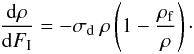 (A.2)This
equation can be used with the IR feature integrated optical depth A
instead of the hydrogen concentration ρ of the material. It is a simply
phenomenological function that does not result from a model.
(A.2)This
equation can be used with the IR feature integrated optical depth A
instead of the hydrogen concentration ρ of the material. It is a simply
phenomenological function that does not result from a model.
Appendix B: Comparison of the recombination model with the exponential fit
We performed the two kinds of fit with our data, based on Eqs. (2) and (A.1), using σd and ρf as adjustable parameters. For all experiments, the best fit based on the bulk molecular recombination (Eq. (2)) has a value of χ2 lower or equal to the one corresponding to the best fit using Eq. (A.1). Therefore, even if the fits using Eq. (A.1) agree well with the experimental data, Eq. (2) provides a better representation of hydrogen concentration in the irradiated films than Eq. (A.1) (see a comparison of the two different best fits determined with each method in Fig. B.1). This is why we use the recombination model results in this article.
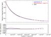 |
Fig. B.1 Comparison between the two different best fits of the hydrogen release induced by ion irradiation. This example corresponds to irradiation by 85 MeV Si7+. |
The uncertainties on the hydrogen release cross section determined by Eq. (2) are greater than those determined with Eq. (A.1) because σd is more dependent on the value of ρf in Eq. (2) than in Eq. (A.1). To reduce these uncertainties, it would be necessary to determine the asymptotic behaviour more precisely and thus irradiate with fluxes that are too high (very far from the interstellar one, and that induce heating of the sample) or during times that are far longer. Such a long time was not possible to reach within the available time on the ion irradiation facility.
Appendix C: Aliphatic C-H destruction parameters determined by the exponential fit
The obtained destruction cross section σd, relative final hydrogen content Af/Ai, and corresponding volume 1/ρf values obtained for the different experiments with the exponential fits are reported in Table C.1. The obtained σd values are plotted as a function of Se in Fig. C.1, for a-C:H and soot samples. As with the recombination model, σd increases with Se as a power law, and this correlation can be fitted by Eq. (5). The corresponding values of α and K are given in Table C.2 for a-C:H and soot. The σd values obtained with the exponential fit are slightly higher than those obtained with the recombination model, but the α possible values obtained with the exponential fit agree with those obtained with the recombination model.
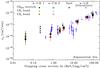 |
Fig. C.1 Aliphatic C-H destruction cross section σd obtained with the exponential fit as a function of the electronic cross section Se for the different ion/energy irradiation of our a-C:H (filled dots for a-C:H 1, and squares for a-C:H 2) and soot (black asterisks) samples. Cross sections calculated from data of different a-C:H irradiation studies are represented with blue diamonds (Adel et al. 1989; Baptista et al. 2004; Baumann et al. 1987; Fujimoto et al. 1988; González-Hernández et al. 1988; Ingram & McCormick 1988; Marée et al. 1996; Mennella et al. 2003; Pawlak et al. 1997; Prawer et al. 1987; Som et al. 2005, 1999; Zou et al. 1988). See text for details. |
In Fig. C.1 we also represented σd values obtained with the exponential fit for a-C:H from data found in the literature (Adel et al. 1989; Baptista et al. 2004; Baumann et al. 1987; Fujimoto et al. 1988; González-Hernández et al. 1988; Ingram & McCormick 1988; Marée et al. 1996; Mennella et al. 2003; Pawlak et al. 1997; Prawer et al. 1987; Som et al. 2005, 1999; Zou et al. 1988). In the article of Pawlak et al. (1997), many σd have been calculated with exponential fits, but data of the hydrogen depletion as a function of the fluence does not appear for most of these experiments. These data appear thus without error bars in Fig. C.1. As in Fig. 4, we did not plot results with Sn/Se > 0.5, or d/Rp > 0.9.
All Tables
Results of ion irradiation experiments obtained with the recombination model fits.
Comparison of the values of η, the ionisation and destruction rates corresponding to the different cosmic ray distribution A/H(Z).
Percentage of destruction %d at a typical cloud time scale t = 3 × 10⁷ yrs for the different fits adopted concerning σd and Af/Ai.
Contribution of each major CR element in the abundance, ionisation, and destruction when Af/Ai = 0 is considered.
Synthetic table giving the characteristic times of destruction and formation processes of the aliphatic hydrogenated carbon component in the different phases of the interstellar medium.
All Figures
|
Fig. 1 Infrared spectra (before irradiation) of the different a-C:H and soot samples: IR spectra of samples a-C:H 1 (thickness d ≈ 10 μm) and a-C:H 2 (d ≈ 7 μm) are in the left panel and the soot IR spectrum is in the right panel (d ≈ 5 μm). Spectrum of a-C:H 1 is offset by 1.5 for a better clarity. |
| In the text | |
|
Fig. 2 Examples of the destruction of the aliphatic C-H stretching IR absorption feature around 2900 cm-1 during ion irradiation of a-C:H 1 a), a-C:H 2 b), and soot c). The upper (red) line is the initial spectrum, before irradiation. The optical depth decreases (from green to purple lines in the online coloured version) as the fluence rises. The fluence between two spectra is of the order of few 1012 and few 1013 ions cm-2 for the Si7+ and C6+ irradiations, respectively. |
| In the text | |
|
Fig. 3 Examples of evolution of the relative integrated optical depth of the aliphatic C-H stretching band with the energy deposited by the ions and the associated fits (recombination model). The deposited energy is calculated from the ion fluence: FE = FI·Se. The a-C:H and soot samples are represented on the left and on the right, respectively. |
| In the text | |
|
Fig. 4 Aliphatic C-H destruction cross section σd obtained with the recombination model as a function of the electronic cross section Se for the different ion/energy irradiation of our a-C:H (filled dots for a-C:H 1, and squares for a-C:H 2) and soot (black asterisks) samples. Cross sections calculated from data of different a-C:H irradiation studies are represented with blue diamonds (Adel et al. 1989; Baptista et al. 2004; Baumann et al. 1987; Fujimoto et al. 1988; González-Hernández et al. 1988; Ingram & McCormick 1988; Marée et al. 1996; Mennella et al. 2003; Pawlak et al. 1997; Prawer et al. 1987; Som et al. 2005, 1999; Zou et al. 1988). See text for details. |
| In the text | |
|
Fig. 5 Aliphatic C-H destruction cross section σd as function of the electronic cross section Se for the different ion/energy irradiation of the a-C:H samples. The values corresponding to the C-H stretching modes at 3.4 μm (in black), the CH2 bending mode at 6.85 μm (in red), and the CH3 bending mode at 7.25 μm (in green) are represented for both a-C:H 1 (filled dots) and a-C:H 2 (squares). The best fit and the fits with extreme values of α are plotted (the corresponding values of α are written). The coloured arrows represent the Se range of the few major cosmic ray elements. |
| In the text | |
|
Fig. 6 Final relative integrated optical depth Af/Ai of C-H stretching modes, obtained after infinite irradiation as function of the electronic cross section Se for the different irradiation ion/energy of a-C:H 1 samples. Two different fits corresponding to the linear increase of the recombination volume V with Se (Eq. (6)) are plotted: the solid line (fit 1) is the best fit, and the dashed line (fit 2) represents an extreme fit for which the asymptotic Af/Ai are the highest for low Se. The coloured arrows represent the Se range of the few major cosmic ray elements. |
| In the text | |
|
Fig. 7 Abundance of elements in cosmic rays as function of their atomic number Z at energies around 0.1−1 GeV/nucleon, normalised to hydrogen (from http://galprop.stanford.edu/, Simpson 1983; Meyer et al. 1998; Fig. 3 of Hörandel 2008, and references therein). |
| In the text | |
|
Fig. 8 Differential flux dN/dEA distribution with the cosmic ray energy per nucleon EA for some of the cosmic ray elements (hydrogen, helium, oxygen, and iron) (Webber & Yushak 1983; Shen et al. 2004). The dotted lines are the values given by GALPROP (http://galprop.stanford.edu/webrun/, Vladimirov et al. 2011). |
| In the text | |
|
Fig. 9 Evolution of the C-H aliphatic component of the interstellar matter under cosmic ray irradiation. The values of σd were determined from a-C:H 1 data with α = 1.0 (see Fig. 5). The black curve corresponds to an exponential decrease without residual hydrogen content taking into account (ρ/ρi = exp(−Rd,CR·t)). The red solid (fit 1) and dashed (fit 2) curves are obtained when the asymptotic values ρf/ρi ≠ 0 are considered. Values of ρf/ρi are determined from a-C:H 1 data and two different fits (see Fig. 6 and text for details). The dotted vertical line corresponds to a typical cloud time scale t = 3 × 10⁷ yr. (McKee 1989; Draine 1990; Jones et al. 1994). |
| In the text | |
|
Fig. 10 Variation of |
| In the text | |
|
Fig. B.1 Comparison between the two different best fits of the hydrogen release induced by ion irradiation. This example corresponds to irradiation by 85 MeV Si7+. |
| In the text | |
|
Fig. C.1 Aliphatic C-H destruction cross section σd obtained with the exponential fit as a function of the electronic cross section Se for the different ion/energy irradiation of our a-C:H (filled dots for a-C:H 1, and squares for a-C:H 2) and soot (black asterisks) samples. Cross sections calculated from data of different a-C:H irradiation studies are represented with blue diamonds (Adel et al. 1989; Baptista et al. 2004; Baumann et al. 1987; Fujimoto et al. 1988; González-Hernández et al. 1988; Ingram & McCormick 1988; Marée et al. 1996; Mennella et al. 2003; Pawlak et al. 1997; Prawer et al. 1987; Som et al. 2005, 1999; Zou et al. 1988). See text for details. |
| In the text | |
Current usage metrics show cumulative count of Article Views (full-text article views including HTML views, PDF and ePub downloads, according to the available data) and Abstracts Views on Vision4Press platform.
Data correspond to usage on the plateform after 2015. The current usage metrics is available 48-96 hours after online publication and is updated daily on week days.
Initial download of the metrics may take a while.