| Issue |
A&A
Volume 529, May 2011
|
|
|---|---|---|
| Article Number | A34 | |
| Number of page(s) | 43 | |
| Section | Interstellar and circumstellar matter | |
| DOI | https://doi.org/10.1051/0004-6361/201015821 | |
| Published online | 28 March 2011 | |
Optical spectroscopic variability of Herbig Ae/Be stars⋆,⋆⋆
1
Centro de Astrobiología, Departamento de Astrofísica (CSIC-INTA), ESAC Campus, PO Box 78, 28691 Villanueva de la Cañada, Madrid, Spain
e-mail: This email address is being protected from spambots. You need JavaScript enabled to view it.
2
Departamento de Física Teórica, Módulo 15, Facultad de Ciencias, Universidad Autónoma de Madrid, PO Box 28049, Cantoblanco, Madrid, Spain
3
GAIA Science Operations Centre, ESA, European Space Astronomy Centre, PO Box 78, 28691 Villanueva de la Cañada, Madrid, Spain
4
School of Physics & Astronomy, University of Leeds, Woodhouse Lane, Leeds LS2 9JT, UK
5
Herschel Science Centre, ESA, European Space Astronomy Centre, PO Box 78, 28691 Villanueva de la Cañada, Madrid, Spain
Received: 26 September 2010
Accepted: 15 February 2011
Abstract
Aims. In order to gain insights into the variability behaviour of the circumstellar (CS) atomic gas, we have analysed 337 multi-epoch optical spectra of 38 Herbig Ae/Be (HAeBe) stars.
Methods. Equivalent widths (EWs) and line fluxes of the Hα, [O i]6300, He i5876 and Na iD lines were obtained for each spectrum; the Hα line width at 10% of peak intensity (W10) and profile shapes were also measured and classified. The mean line strengths and relative variabilities were quantified for each star. Simultaneous optical photometry was used to estimate the line fluxes.
Results. We present a homogeneous spectroscopic database of HAeBe stars. The lines are variable in practically all stars and timescales, although 30% of the objects show a constant EW in [O i]6300, which is also the only line that shows no variability on timescales of hours. The He i5876 and Na iD EW relative variabilities are typically the largest, followed by those in [O i]6300 and Hα. The EW changes can be larger than one order of magnitude for the He i5876 line, and up to a factor 4 for Hα. The [O i]6300 and HαEW relative variabilities are correlated for most stars in the sample. The Hα mean EW and W10 are uncorrelated, as are their relative variabilities. The Hα profile changes in ~70% of the objects. The massive stars in the sample (M∗ > 3 M⊙) usually show more stable Hα profiles with blueshifted self-absorptions and less variable 10% widths.
Conclusions. Our data suggest multiple causes for the different line variations, but the [O i]6300 and Hα variability must share a similar origin in many objects. The physical mechanism responsible for the Hα line broadening does not depend on the amount of emission; unlike in lower-mass stars, physical properties based on the Hα luminosity and W10 would significantly differ. Our results provide additional support to previous works that reported different physical mechanisms in Herbig Ae and Herbig Be stars. The multi-epoch observations we present are a useful tool for understanding the origin of the CS lines and their variability, and to establish distinctions in the physical processes operating in pre-main sequence stars.
Key words: stars: pre-main sequence / stars: activity / circumstellar matter / accretion, accretion disks / protoplanetary disks
Based on observations carried out by the EXPORT consortium.
Appendices are only available in electronic form at http://www.aanda.org
© ESO, 2011
1. Introduction
Herbig Ae and Be (HAeBe) stars are intermediate mass, pre-main sequence (PMS) objects, which are considered as the possible progenitors of Vega-like stars surrounded by circumstellar (CS) debris disks and, eventually, planets. The spectroscopic monitoring of some sources (see e.g. Praderie et al. 1986; Pogodin 1994; Rodgers et al. 2002; Mora et al. 2002, 2004) revealed that the spectra of HAeBe objects are not only characterized by the presence of emission lines, but also by the complex variations observed in both the emission and absorption features. This variability is also characteristic of T-Tauri stars (see e.g. Johns & Basri 1995; Schisano et al. 2009, and references therein).
The optical spectra of PMS stars show several important features that have been related to different physical processes. Magnetospheric accretion models have succeeded in reproducing the profiles and strengths of the Hα and Na iD lines (Hartmann et al. 1994; Muzerolle et al. 1998a,b, 2001, 2004). Despite the unknown nature of the magnetic fields in HAeBe stars (see e.g. Wade et al. 2005; Alecian et al. 2007; Wade et al. 2007; Hubrig et al. 2009), magnetospheric accretion has been shown to act in several HAe objects (Muzerolle et al. 2004; Mottram et al. 2007). The Hα line has also been associated with winds (Cabrit et al. 1990) or with combined magnetopheric accretion-wind models (Kurosawa et al. 2006). The Hα line width at 10% of peak intensity is used to estimate accretion rates in lower-mass PMS stars (see e.g. White & Basri 2003; Natta et al. 2004; Jayawardhana et al. 2006). The [O i]6300 line has been associated with accretion-powered outflows and winds (Finkenzeller 1985; Böhm & Catala 1994; Böhm & Hirth 1997; Corcoran & Ray 1997, 1998), and with the stellar UV-luminosity and disk-shape (Acke et al. 2005; van der Plas et al. 2008). The high temperature close to the stellar surface, which is generated in the accretion shock, has been suggested to be responsible for the He i5876 line (Tambovtseva et al. 1999; Grinin et al. 2001). Na iD lines seen in absorption describe the complex gas motions characterizing the CS medium around PMS stars (Mora et al. 2002, 2004).
Most spectroscopic studies are based on isolated spectra of different sources or have been focused on particular objects. The different approaches explaining the physical origin of the lines can profit from multi-epoch spectroscopic data. The EXPORT consortium (Eiroa et al. 2000) monitored a large number of intermediate-mass PMS stars, allowing for an extensive and homogeneous study of their spectroscopic variability. In this paper we analyse EXPORT multi-epoch optical spectra of HAeBe stars, specifically the lines Hα, [O i]6300, He i5876, Na i D25890 and D15896. The photometric and spectroscopic variability of those objects requires simultaneous measurements to obtain accurate values for the line fluxes. These are derived using the already published simultaneous optical photometry of the stars in our sample (Oudmaijer et al. 2001). We will present a dataset comprised of multi-epoch line equivalent widths, fluxes, Hα profiles and widths, which is provided as a valuable observational legacy of the spectroscopic behaviour of HAeBe stars. We analyse and quantify the observed changes in the different lines and look for general trends, mainly focused on the equivalent width variability. A more specific analysis will be made in subsequent papers.
Section 2 describes the sample and spectra. Section 3 presents our results. They are analysed in Sect. 4, which describes the spectroscopic variability shown by the different lines (Sect. 4.1 for Hα, Sect. 4.2 for [O i]6300, Sect. 4.3 for He i5876, Sect. 4.4 for Na iD and Sect. 4.5 for a compendium of the spectroscopic characterization). Section 5 discusses the results and Sect. 6 includes a brief summary and conclusions.
2. Sample properties and observations
Table 1 (left side) shows the 38 stars in the sample. Columns 1 to 3 indicate the name of the star, the spectral type, and the stellar mass. While most of the objects are HAeBe stars (covering almost all these objects in the Northern hemisphere from the catalogue of Thé et al. 1994), 10 of them have spectral types ranging from F3 to G1. The stellar masses range between ~1−6 M⊙. As a selection criterion, all objects show the Hα line in emission. The sample span the 1 − 15 Myr age-range (Manoj et al. 2006; Montesinos et al. 2009), which is the period of the evolution from protoplanetary to young debris disks and the epoch of planet formation. There is a good balance between variable and non-variable objects, according to their simultaneous photopolarimetric behaviour (Oudmaijer et al. 2001; Eiroa et al. 2001, 2002).
The spectra were obtained by the EXPORT consortium (Eiroa et al. 2000) with the long slit Intermediate Dispersion Spectrograph (IDS) on the 2.5 m Isaac Newton Telescope (INT). The typical spectral resolution is R ~ 5500, covering the wavelength range λλ 5800–6700 Å. The slit width was 1′′ projected on the sky (i.e. narrow enough to avoid confusion in most binaries of the sample; see e.g. Wheelwright et al. 2010, and references therein). Details of the observations and data reduction are given by Mora et al. (2001). The stars were observed over one or more of the four EXPORT runs. The right side of Table 1 shows the log of the observations, illustrating the monitoring timescales: from days to months in general, and for a few stars even hours. A total of 337 spectra were obtained, ranging from 3 to 18 per star, typically 6–10 spectra per object. In order to study the non-photospheric contribution (see Sect. 3), additional spectra of 28 spectroscopic standard MS stars were also taken in the same campaigns and with the same configuration.
Sample of stars and log of the INT/IDS spectra analysed.
3. Results
The contribution of the CS component to the spectra of the PMS sample was estimated from the spectra of the standard MS stars with similar spectral types. These were rotationally broadened using the projected rotational velocities derived by Mora et al. (2001) for the PMS objects. The non-photospheric contribution is given by the residuals obtained from the subtraction of the broadened standard spectra from the observed PMS spectra. The results refer to the normalized non-photospheric spectra.
Table A.1 gives estimates of the equivalent widths (EWs) of the Hα, [O i]6300, He i5876, Na iD2 and Na iD1 lines for all spectra of our sample. The Hα widths at 10% of peak intensity (W10) and profile types (see below) are also listed. As usual, positive and negative EW values correspond to absorption and emission features, respectively. When a spectral line is seen partly in absorption and partly in emission, only the strongest component (i.e., that with the largest |EW|) is included. This double contribution appears mainly in the He i5876 line, which usually shows both a redshifted absorption and a blueshifted emission. Although a specific analysis of this behaviour is beyond the scope of this work, it probably indicates the presence of hot infalling gas close to the stellar surface. In addition, the He i5876 and Na iD lines change from absorption to emission in several objects.
Conservative EW uncertainties were estimated by determining the maximum and minimum EW values from two different continuum levels that are located below and above unity (~1 ∓ 1.5σ), respectively. Both continuum levels bracket the adjacent noise to each spectral line. Typical median uncertainties are 3%, 8%, 10%, 20% and 30% of the EW values in the Hα, Na iD2, Na iD1, He i5876 and [O i]6300 lines, respectively. Typical EW-uncertainties are larger than, or similar to, the typical strength of telluric absorption lines (see e.g. Caccin et al. 1985; Lundström et al. 1991; Reipurth et al. 1996). Telluric variability is also in general negligible compared with that reported for the lines (see below). Uncertainties for W10 are typically ~ 1% of its value.
We follow the two-dimensional scheme by Reipurth et al. (1996) to classify the observed Hα profiles: type I are symmetric with no or very weak dips; type II are double-peaked profiles with the secondary peak higher than half the strength of the primary; type III have a secondary peak less than half the strength of the primary and type IV are P Cygni-type profiles. The scheme incorporates the designations “R” or “B” to indicate if the secondary peak is redshifted or blueshifted with respect to the primary. If both peaks have equal strengths, only the profile type is indicated. For type IV, the letters indicate a P-Cygni profile (“B”) or inverse P Cygni (“R”). The letter “m” is added when more than one absorption appears, and also when small dips are apparent in the type I profiles.
An object is considered as “variable” in the EW of a line when its value differs in two or more spectra, taking into account the individual uncertainties. We use the relative variability | σ(EW)/ ⟨ EW ⟩ | as a reliable measurement of the strength of the EW-changes, where σ is the standard deviation from the individual EW measurements of a given star1 and ⟨ EW ⟩ is the mean line equivalent width. Johns & Basri (1995) used an equivalent parameter to characterize the variability of the Hα intensity in several T-Tauri stars. The non-variable objects tend to show the lowest values of | σ(EW)/ ⟨ EW ⟩ | ; in these stars this ratio only contains information about the precision of the measurements. σ(W10)/ ⟨ W10 ⟩ and σ(L)/ ⟨ L ⟩ are used to assess the relative variability of the Hα line width and that of the line luminosities.
Table 2 gives the mean line equivalent widths and their relative variabilities. Mean values and relative variabilities of W10(Hα) are also given, as well as the number of spectra displaying the corresponding Hα profiles. Uncertainties are listed for the non-variable stars in a given spectral line.
Mean equivalent and line widths, relative variabilities, and Hα profiles.
Table A.2 shows the line fluxes for the spectra with simultaneous optical photometry (Oudmaijer et al. 2001). They were estimated using the EWs in Table A.1, and the V and R magnitudes obtained during the same night, taken within a time span of less than 2 − 3 h. Fluxes are derived for 137 spectra (i.e. 41% of the initial 337 spectra) of 36 stars (the initial sample excluding AS 442 and R Mon). We used the expression F = F0 × |EW|/100.4m, with F0 the zero-magnitude fluxes (Bessell 1979) and m the V (for the Na iD and He i5876 lines) or R (for the Hα and [O i]6300 lines) magnitudes. We also computed fluxes for the Na iD and He i5876 lines that showed positive EWs, meaning the stellar flux absorbed by the lines. These fluxes are related to the amount of gas in the line of sight, traced by these species.
Table 3 shows the typical (mean) line luminosities of each star, obtained by averaging the fluxes in Table A.2 and assuming spherical symmetry. The distances considered are indicated in Col. 3. The line luminosity relative variabilities are also given, although the statistics is poorer than for the EWs, because of the lower number of spectra with simultaneous photometry (given in Col. 2).
Mean line luminosities.
The reddening towards the objects is low for most stars, with very few exceptions (E(B − V) ≤ 0.1 for almost half of the objects, and E(B − V) ~ 1 for the most reddened sources – V1686 Cyg and LkHa 234 –, Merín 2004). The fact that our multi-epoch line fluxes and luminosities are not de-reddened avoids introducing additional uncertainties and does not affect the analysis and discussion in the following sections.
4. Analysis
4.1. The Hα line
Our data show that the Hα emission line remains constant, at least on timescales of days-months, for HD 141569 and 51 Oph, based on 8 and 10 spectra, respectively. In addition, Hα is non-variable in HD 58647, R Mon and VY Mon; however, there are only three spectra per object, so that variability at timescales longer than days cannot be excluded. The remaining stars show EW(Hα) variability.
The typical Hα relative variability, |σ/ ⟨ EW ⟩|, is 0.19 (mean) and 0.15 (median)2. HαEW variations up to a factor EWmax/EWmin ~ 4 can be observed for individual stars (e.g. V1686 Cyg, VX Cas). The ⟨ EW ⟩ (Hα) ranges between −2 and −74 Å, with typical values of −19.4 Å (mean) and −14.4 Å (median)
All objects change their W10(Hα) but HD 58647 with only three measurements and V346 Ori with very large uncertainties. The typical relative variability is only σ(W10)/ ⟨ W10 ⟩ = 0.09 (mean), 0.07 (median). Some stars show W10(Hα) changes up to a factor ~ 2.5 (e.g. CQ Tau). The ⟨ W10 ⟩ (Hα) ranges from 355 km s-1 to 908 km s-1 and is typically around 640 km s-1 Changes of both EW and W10 are seen on timescales as short as hours from the five objects with more than one spectrum per night. Our data show typical changes of a factor ~ 1.1 in both parameters on this timescale. The strongest variations occur over longer timescales however, i.e. weeks-months, at least in our database.
Variations in the line profile are very frequent – only 18% of the stars display the same type in all spectra – and are common on timescales of days; ~ 73% show variations from one day to the next one. Some extreme cases are VV Ser, changing from type IIR to type IIB profiles practically from spectrum to spectrum, and UX Ori, BO Cep and BH Cep, which show five different profile types. BH Cep also shows the fastest variation, changing from IIB to IIIB in less than one hour. The high-mass objects in our sample tend to show the same Hα profile type during a given observing run, i.e. on timescales of a week, and all objects showing stable Hα profiles only on shorter timescales have M∗ < 3 M⊙.
All Hα profiles classified by Reipurth et al. (1996) are observed in our spectra with a similar distribution (see also Vieira et al. 2003): type II profiles are the most frequent (52% of the observations), followed by type III (32%) and I (13%). P-Cygni type profiles are the least common (less than 3%). “R” and “B” profiles appear almost in the same proportion (44% versus 43%). However, B profiles are mainly shown by the most massive objects in our sample (the stars with M∗ ≥ 3M⊙ have “B” profiles in 60% of the spectra; in fact only they show P-Cygni signatures). “R” profiles dominate in the HAe and lower-mass range of our sample (47% of the spectra, against 37% in “B”).
4.2. The [OI]6300 line
Thirty-two out of the 38 stars show the [O i]6300 emission line. The line is variable in ~ 70% of the stars; typical values of | σ/ ⟨ EW ⟩ | are 0.51 (mean) and 0.26 (median). The largest EW variations – a factor ~ 7 − 9 – are seen, as for the Hα line, in V1686 Cyg and VX Cas. [O i]6300 variability is not detected on timescales of hours. For seven objects, the line is seen only in several spectra. The emission is very faint in these stars and their | σ/ ⟨ EW ⟩ | values should be taken with caution. They could be affected by telluric variability or by artefacts from the telluric emission subtraction. Higher SNR spectra of the objects with the weakest [O i]6300 line would be necessary to better estimate their line relative variability. Typical ⟨ EW([O i]6300) ⟩ values are − 0.29 Å (mean) and − 0.12 Å (median). The difference between the mean and median values comes from the few objects showing | ⟨ EW([O i]6300) ⟩ | ≫ 1 Å.
Most of the stars display a single-peaked almost symmetric low-velocity component. For the few objects with profiles different from single-peaked, the emission tends to be faint and the SNR low, probably distorting their profiles.
4.3. The He I 5876 line
Only 4 out of the 38 stars do not show the He i5876 line in any of their spectra. The line is present in the rest of the stars, although five objects do not show it in all their spectra. In seven stars the line appears either in absorption or in emission, depending on the observing date. In most cases, 84% of the objects, the line is present either fully in absorption, or the absorption is dominant. All objects show variations in the EW of the line, with the exception of HD 150193, HD 58647, and R Mon. There are only three spectra available for each object, thus we cannot exclude that this result is due to the comparatively poor spectroscopic coverage.
Changes in EW(He i5876) take place in all timescales. The relative variability range is 0.12 < | σ/ ⟨ EW ⟩ | < 1.22, with a typical value of 0.53 (mean) and 0.46 (median). The variability is larger in those objects where the line is dominated by absorption. Line EW variations up to a factor EWmax/EWmin ~ 13 can be observed in these cases (e.g. BO Cep), compared to a factor ~ 6 for the objects showing the line emission (e.g. HD 144432). The typical mean and median value of | ⟨ EW(He i5876) ⟩ | is 0.38 Å, ranging between − 0.47 ≤ ⟨ EW(He i5876) ⟩ ≤ 0.81 Å.
4.4. The Na ID lines
Na iD lines are seen in absorption for most of the cases (~70% of the stars). The Na iD absorption lines can have a non-negligible interstellar contribution owing to clouds in the line of sight of our objects (see e.g. Redfield 2007). Therefore, several EWs given in Tables A.1 and 2 should be considered as upper limits to the CS absorption. The timescale variability of the interstellar absorption is, however, much longer than that covered by our spectra (see e.g. Lauroesch & Meyer 2003). Thus, the observed variability of the Na iD lines is caused by the CS gas component.
There are seven objects with a constant EW in the Na iD lines. Again, apart from HD 34700 and HD 190073, only three spectra are available for each one. The remaining objects show EW variability. As expected, the relative variability is equal in both Na iD lines (~0.50), within the uncertainties. As for the He i5876 line, the smallest EWmax/EWmin factors are shown by the objects with Na iD in emission (up to a a factor ~4 in e.g. HD 163296, against a factor ~6 for objects with the lines in absorption such as CO Ori). Na iD EWs do not usually change in hours. The only exception is HD 163296; its Na iD emission changed a factor ~2 in one night (29-Jul.-1998), but no variations were detected the two following nights. We note that variations on timescales of hours have been reported for UX Ori using higher resolution spectra (Mora et al. 2002). The typical ⟨ EW(Na iD) ⟩ in our sample is ~0.40 Å.
The Na iD ratio is a good indicator of the optical thickness at these wavelengths (e.g. Mora et al. 2002, 2004). Changes in the optical depth of the CS medium in the line of sight are observed in almost all objects, however, averaged values indicate optically thick media for most of the stars ( ⟨ EW(Na iD2)/EW(Na iD1) ⟩ ~ 1).
4.5. Compendium of the EW variability
Table 4 summarizes typical values for the equivalent widths and their relative variabilities, the minimum and maximum values, the percentage of objects showing line variations, and the number of objects with variability on a timescale of hours. We remark that this one refers only to a sample of five stars with that spectroscopic timescale coverage. The percentage of objects where the corresponding line is undetected is also given. The values in the last three rows of the bottom panel are derived considering both Na iD lines.
Summary of the typical equivalent and line widths and their relative variability.
In general, CS absorption features show a larger EW variability than the emission lines. The EW relative variability is significantly higher for the He i5876, Na iD and [O i]6300 lines than for Hα. In addition, approximately 30% of the objects show a constant [O i]6300 equivalent width, but the remaining lines are variable in practically all stars in which these are detected. Considering the short timescale variations, the number of variable stars is similar for the He i5876 and Hα lines, a small percentage seems to present Na iD variability, while no star shows changes in [O i]6300.
Finally, when simultaneous EWs and line fluxes are compared, the relative variability of the EWs tends to be equal to or an upper limit of that of the line fluxes for most of the stars.
5. Discussion
The described results indicate that the physical conditions in the line-forming regions are highly complex and variable on practically any timescale, and that the use of individual EW or line flux measurements could lead to biased conclusions. Averaged EW values are likely more representative, which might be specially true for the absorption component of the He i5876 line, where the variations can be larger than one order of magnitude. Our sample shows that there is no significant correlation between the mean strengths and their relative variabilities, therefore, both are necessary to completely characterize the line behaviour of the stars.
Although a detailed study of the physical origin of the lines and their variations is beyond the scope of this work, the observed differences between the typical variabilities of the features, both in strength and in timescale, suggest multiple causes for the different line variations. In addition, our results show that there are no clear correlations among the relative variabilities of the different lines, excluding the obvious relation between the Na iD2 and D1 changes, and the one between Hα and [O i]6300. Figure 1 shows the Hα and [O i]6300 EW relative variabilities of the sources with a clear detection of the [O i] line in all their spectra (this avoids possible telluric/instrumental effects; see Sect. 4.2). The Spearman’s probability of false correlation (see e.g. Conover 1980) is only 0.19%. Although | σ/ ⟨ EW ⟩ | ([O i]6300) tends to be larger than | σ/ ⟨ EW ⟩ | (Hα), the strength of the corresponding EW variations are coupled in many stars. This suggests that the EW variations share a common origin. One possibility is that Hα and [O i]6300 are affected by accretion-wind variability (see below and e.g. Corcoran & Ray 1997, 1998). Variability in the UV radiation would have influence on the strength of the [O i]6300 emission (Acke et al. 2005). Changes in the stellar continuum level could also affect the EW variations of both lines simultaneously, as we outline below.
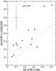 |
Fig. 1 Equivalent width relative variability of the [O i]6300 line against that in Hα for the objects showing clear [O i] detections in all their spectra. The dotted line indicates equal values. The typical error bars and the Spearman’s probability of false correlation are indicated. |
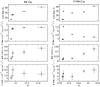 |
Fig. 2 Equivalent widths and line fluxes of the Hα and [O i]6300 lines against the simultaneous V magnitude (Oudmaijer et al. 2001) for RR Tau and V1686 Cyg. |
Line EWs change because the conditions in the CS gas vary (producing variations in the line luminosity) and/or because there are changes in the continuum level. Most objects with significant V-band variability (ΔV ≥ 0.4) increase their Hα and [O i]6300 EWs as the stellar brightness decreases, leaving the corresponding line luminosities almost constant or even decreasing (see e.g. RR Tau on the left panel of Fig. 2, and also Rodgers et al. 2002). This behaviour has been explained as due to the coronographic effect caused by dusty clouds that occult the stellar surface (Grinin et al. 1994; Rodgers et al. 2002). The EW enhancement would result from the contrast between the continuum dimming and the almost constant line luminosity. This explanation has been suggested for stars showing the UXOr behaviour, but we note that objects such as V1686 Cyg, which is not classified as an UXOr from its simultaneous optical photopolarimetry (Oudmaijer et al. 2001), show a similar pattern in the Hα and [O i]6300 lines (see right panel of Fig. 2).
Continuum changes can be rejected as the origin of the EW variability in other cases. Several examples are given in Fig. 3, where the remarkable line variations are not accompanied by significant changes in the simultaneous optical brightness (Oudmaijer et al. 2001). The main spectroscopic features shown by HK Ori during two consecutive nights are plotted in the top panels. The appearance of redshifted Na iD emission lines is accompanied by a decrease of the absorption component of the He i5876 line. Simultaneously, the [O i]6300 and Hα lines reduce their luminosities by a factor ~ 3. Hα changes from double-peaked to a redshifted single-peaked profile, with W10 remaining constant. The corresponding Na iD ratios indicate that the CS gas changed from optically thick to optically thin at these wavelengths. These findings are difficult to interpret, but obscuring dusty screens in the line of sight are clearly excluded. An alternative could be that the accretion and/or wind rate diminished from one night to the other and produced the decrease of the Hα and [O i] strengths and reduced the gas density, which explains the change to optically thin. This would allow the detection of hot infalling gas very close to the stellar surface, seen in emission. The examples in the middle and bottom panels of Fig. 3 show that small variations in the Hα and [O i]6300 lines are again related to each other.
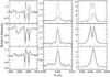 |
Fig. 3 Na iD and He i5876 (left panels), [O i]6300 (middle panels) and Hα (right panels) lines shown by HK Ori (top panels, 1998, October 25 and 26), VV Ser (middle panels, 1998, October 24 and 27) and CO Ori (bottom panels, 1998, October 25 and 26). The dashed and solid lines correspond to the first and second night. |
The data show that the main origin for the EW-variability (gas or continuum changes) strictly depends on each star, each line considered and the epoch of observation. The complex behaviour of the lines and the continuum requires their simultaneous characterization to distinguish the origin of the spectroscopic variability.
Regarding the Hα line, its relative variability in W10 is twice as low as that in the EW, and we find no significant correlation either between the mean widths and line strengths or between their relative variabilities. Figure 4 shows that these parameters have a very high Spearman’s probability of false correlation. This suggests that the physical mechanism responsible for the Hα broadening does not depend on the column density of hydrogen atoms. A similar result was found for the [OI]6300 line by Acke et al. (2005). Both the Hα luminosity and W10 are used as empirical accretion tracers in lower-mass stars (see e.g. Fang et al. 2009; Jayawardhana et al. 2006, and references therein). Our result indicates that both Hα measurements would typically produce different estimates in HAeBe stars.
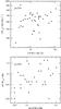 |
Fig. 4 Mean value of the width of the Hα line against that of the equivalent width (top) and relative variabilities (bottom). Triangles are lower limits for ⟨ W10(Hα) ⟩ . The Spearman’s probabilities of false correlation are indicated. |
Finally, we stress that the Hα behaviour depends on the stellar mass. The more massive objects in our sample tend to have more stable Hα line profiles with blueshifted self-absorptions, which could be indicative of a strong wind contribution (see also e.g. Finkenzeller & Mundt 1984). The less massive stars in our sample are slightly dominated by redshifted self-absorptions in their Hα profiles, which suggests that they are influenced by accretion (Muzerolle et al. 2004). In addition, our multi-epoch data suggest that the strength of the W10(Hα) variability is significantly anti-correlated with the mass of the central object. Figure 5 shows our σ/ ⟨ W10(Hα) ⟩ estimates against the stellar mass. Despite the scatter at low masses, almost all stars with M∗ ≥ 3.0 M⊙ show a low W10(Hα) relative variability ( ≤ 0.06). A more extended emitting region could produce more stability in the line width. Preliminary magnetospheric accretion modelling that we are currently applying on HAe stars suggests that changes in the size of the magnetosphere and/or in the gas temperature of this region could induce significant changes in W10(Hα) (hundreds of km s-1). The results found point to different physical processes operating in Herbig Ae and Herbig Be stars, which agrees with previous spectropolarimetric studies (see e.g. Vink et al. 2002; Mottram et al. 2007).
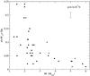 |
Fig. 5 Relative variability of the Hα width at 10% of peak intensity against the stellar mass. Triangles are upper and lower limits for M∗. The typical σ/ ⟨ W10(Hα) ⟩ uncertainty and the Spearman’s probability of false correlation are indicated. |
6. Summary and conclusions
The work presented here shows that multi-epoch spectroscopic observations together with simultaneous photometry are an extremely useful tool to better understand the variability of the circumstellar lines in PMS stars. By means of a large number of optical spectra the variability of the Hα, [O i]6300, He i5876 and Na iD lines has been analysed in a sample of 38 HAeBe stars. These spectra and the simultaneous photometry have allowed us to estimate line fluxes and to soundly assess if the observed EW variations are caused by changes in the stellar continuum or by variations of the circumstellar gas itself. Indeed, the spectra and photometry -and their simultaneous character- on which the analysis is based constitute one of the largest existing data bases to study some of the variability properties in intermediate-mass PMS stars. Several specific results we obtained are:
-
The EW variability of the different lines depends on the analysed timescale and is independent of the mean line strength. The He i587 and Na iD lines show the largest EW variations and can be seen either in absorption or in emission. In contrast, [O i]6300 is the only line without variations on timescales of hours and is also the line with variability in a smaller percentage of the stars in the sample.
-
There is a correlation between the Hα and [O i]6300 relative variabilities, which suggest a common origin. In some stars the EW variability of both lines are due to variations of the continuum, but in other objects the EW variability reflects variations of the line luminosities and, consequently, in the CS gas properties.
-
Mean values and relative variabilities of the Hα line width W10 and EW are uncorrelated in our sample. The lack of correlation between both parameters suggests that Hα broadening does not depend on the column density of hydrogen atoms. Thus, estimates of gas properties, such as accretion rates, based on the HαW10 or EW would differ significantly, unlike in lower mass stars.
-
The Hα behaviour differs depending on the stellar mass, which suggests different physical processes for Herbig Ae and Herbig Be stars. The massive stars tend to show stable Hα profiles, mainly dominated by blueshifted self-absorptions. In addition, stars with M∗ ≥ 3.0 M⊙ show very low W10(Hα) relative variabilities ( ≤ 0.06).
Finally, we point out that in addition to the mean spectra and relative variability distributions available in Appendix B any of the spectra can be requested from the authors and will also be available from Virtual Observatory tools soon.
Online material
Appendix A: Tables with multi-epoch line EWs and fluxes
Equivalent widths, Hα widths at 10% of peak intensity and Hα profile types on different observing Julian Dates.
Line fluxes on several observing Julian Dates for a subsample of the stars.
Appendix B: Mean spectra and relative variability distributions
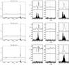 |
Fig. B.1 For each star and observing campaign, the mean spectra and relative variability distributions are plotted on the left side. The HeI5876, NaID, [OI]6300 and Hα regions are enlarged on the right side, for a better visualization. The mean spectrum is given by |


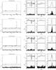 |
Fig. B.1 continued. |
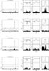 |
Fig. B.1 continued. |
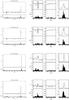 |
Fig. B.1 continued. |
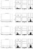 |
Fig. B.1 continued. |
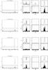 |
Fig. B.1 continued. |
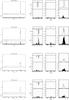 |
Fig. B.1 continued. |
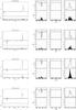 |
Fig. B.1 continued. |
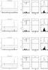 |
Fig. B.1 continued. |
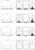 |
Fig. B.1 continued. |
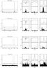 |
Fig. B.1 continued. |
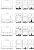 |
Fig. B.1 continued. |
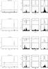 |
Fig. B.1 continued. |
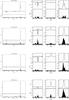 |
Fig. B.1 continued. |
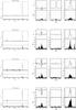 |
Fig. B.1 continued. |
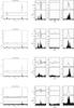 |
Fig. B.1 continued. |
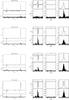 |
Fig. B.1 continued. |
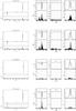 |
Fig. B.1 continued. |
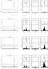 |
Fig. B.1 continued. |
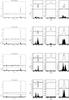 |
Fig. B.1 continued. |
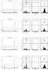 |
Fig. B.1 continued. |
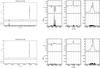 |
Fig. B.1 continued. |
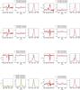 |
Fig. B.2 Individual spectra taken within a time span of hours (i.e. during the same night) for the five objects monitored on this timescale. |
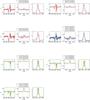 |
Fig. B.2 continued. |
I.e. for N spectra, ![Mathematical equation: \hbox{$\sigma = [\frac{1}{N-1} \sum _{i=1}^N {( EW _i -\langle EW \rangle ) ^2 }] ^{1/2}$}](/articles/aa/full_html/2011/05/aa15821-10/aa15821-10-eq114.png) .
.
In order to improve the reliability of the typical values and ranges derived, the 33 objects with 5 or more spectra are usually taken as a reference.
Acknowledgments
C. Eiroa, G. Meeus, I. Mendigutía and B. Montesinos are partially supported by grant AYA-2008 01727. We thank Enrique Solano and Mauro López for making the spectra available from VO tools.
References
- Acke, B., van den Ancker, M. E., Dullemond, C. P. 2005, A&A, 436, 209 [NASA ADS] [CrossRef] [EDP Sciences] [Google Scholar]
- Alecian, E., Wade, G. A., Catala, C., et al. 2007, IAUS, 243, 43 [NASA ADS] [Google Scholar]
- Alonso-Albi, T., Fuente, A., Bachiller, R., et al. 2009, A&A, 117, 136 [Google Scholar]
- Bessell, M. S. 1979, PASP, 91, 589 [NASA ADS] [CrossRef] [Google Scholar]
- Blondel, P. F. C., Djie, H. R. E., & Tjin, A. 2006, A&A, 456, 1045B [NASA ADS] [CrossRef] [EDP Sciences] [Google Scholar]
- Böhm, T., & Catala, C. 1994, A&A, 290, 167 [NASA ADS] [Google Scholar]
- Böhm, T., & Hirth, G. A. 1997, A&A, 324, 177 [NASA ADS] [Google Scholar]
- Cabrit, S., Edwards, S., Strom, S. E., & Strom, K. M. 1990, ApJ, 354, 687 [NASA ADS] [CrossRef] [Google Scholar]
- Caccin, B., Cavallini, F., Ceppatelli, G., Righini, A., & Sambuco, A. M. 1985, A&A, 149, 357 [NASA ADS] [Google Scholar]
- Conover, W. J. 1980, Practical non-parametric statistics, 2nd edn. (New York: Wiley) [Google Scholar]
- Corcoran, M., & Ray, T. P. 1997, A&A, 321, 189 [NASA ADS] [Google Scholar]
- Corcoran, M., & Ray, T. P. 1998, A&A, 331, 147 [NASA ADS] [Google Scholar]
- Eiroa, C., Alberdi, A., Camron, A., et al. 2000, ESASP, 451, 189 [NASA ADS] [Google Scholar]
- Eiroa, C., Garzón, F., Alberdi, A., et al. 2001, A&A, 365, 110E [NASA ADS] [CrossRef] [EDP Sciences] [Google Scholar]
- Eiroa, C., Oudmaijer, R. D., Davies, J. K., et al. 2002, A&A, 384, 1038 [NASA ADS] [CrossRef] [EDP Sciences] [Google Scholar]
- Fang, M., van Boekel, R., Wang, W., et al. 2009, A&A, 504, 461 [NASA ADS] [CrossRef] [EDP Sciences] [Google Scholar]
- Finkenzeller, U. 1985, A&A, 151, 340 [NASA ADS] [Google Scholar]
- Finkenzeller, U., & Mundt, R. 1984, A&AS, 55, 109 [NASA ADS] [Google Scholar]
- Garcia Lopez, R., Natta, A., Testi, L., & Habart, E. 2006, A&A, 459, 837G [NASA ADS] [CrossRef] [EDP Sciences] [Google Scholar]
- Grinin, V. P., The, P. S., de Winter, D., et al. 1994, A&A, 292, 165 [NASA ADS] [Google Scholar]
- Grinin, V. P., Kozlova, O. V., Natta, A., et al. 2001, A&A, 379, 482 [NASA ADS] [CrossRef] [EDP Sciences] [Google Scholar]
- Hartmann, L., Hewett, R., & Calvet, N. 1994, ApJ, 426, 669 [NASA ADS] [CrossRef] [Google Scholar]
- Hubrig, S., Stelzer, B., Schöller, M., et al. 2009, A&A, 502, 283 [NASA ADS] [CrossRef] [EDP Sciences] [Google Scholar]
- Jayawardhana, R., Coffey, J., Scholz, A., Brandeker, A., & van Kerkwijk, M. H. 2006, ApJ, 648, 1206 [NASA ADS] [CrossRef] [Google Scholar]
- Johns, C. M., & Basri, G. 1995, AJ, 109, 2800 [NASA ADS] [CrossRef] [Google Scholar]
- Kurosawa, R., Harries, T. J., & Symington, N. H. 2006, MNRAS, 370, 580 [NASA ADS] [CrossRef] [Google Scholar]
- Lauroesch, J. T., & Meyer, D. M. 2003, ApJ, 591, L123 [NASA ADS] [CrossRef] [Google Scholar]
- Lundström, I., Arderberg, A., Maurice, E., & Lindgren, H. 1991, A&AS, 91, 199 [NASA ADS] [Google Scholar]
- Manoj, P., Bhatt, H. C., Maheswar, G., & Muneer, S. 2006, ApJ, 653, 657 [NASA ADS] [CrossRef] [Google Scholar]
- Merín, B. 2004, PhD Thesis, Universidad Autónoma de Madrid [Google Scholar]
- Montesinos, B., Eiroa, C., Merín, B., & Mora, A. 2009, A&A, 495, 901 [NASA ADS] [CrossRef] [EDP Sciences] [Google Scholar]
- Mora, A., Merín, B., Solano, E., et al. 2001, A&A, 378, 116 [NASA ADS] [CrossRef] [EDP Sciences] [Google Scholar]
- Mora, A., Natta, A., Eiroa, C., et al. 2002, A&A, 393, 259 [NASA ADS] [CrossRef] [EDP Sciences] [Google Scholar]
- Mora, A., Eiroa, C., Natta, A., et al. 2004, A&A, 419, 225 [NASA ADS] [CrossRef] [EDP Sciences] [Google Scholar]
- Mottram, J. C., Vink, J. S., Oudmaijer, R. D., & Patel, M. 2007, MNRAS, 377, 1363 [NASA ADS] [CrossRef] [Google Scholar]
- Muzerolle, J., Hartmann, L., & Calvet, N. 1998a, AJ, 116, 455 [NASA ADS] [CrossRef] [Google Scholar]
- Muzerolle, J., Calvet, N., & Hartmann, L. 1998b, ApJ, 492, 743 [NASA ADS] [CrossRef] [Google Scholar]
- Muzerolle, J., Calvet, N., & Hartmann, L. 2001, ApJ, 550, 944 [NASA ADS] [CrossRef] [Google Scholar]
- Muzerolle, J., D’Alessio, P., Calvet, N., & Hartmann, L. 2004, ApJ, 617, 406 [NASA ADS] [CrossRef] [Google Scholar]
- Natta, A., Testi, L., Muzerolle, J., et al. 2004, A&A, 424, 603 [NASA ADS] [CrossRef] [EDP Sciences] [Google Scholar]
- Oudmaijer, R. D., Palacios, J., Eiroa, C., et al. 2001, A&A, 379, 564 [NASA ADS] [CrossRef] [EDP Sciences] [Google Scholar]
- Pogodin, M. A., 1994, A&A, 282, 141 [NASA ADS] [Google Scholar]
- Praderie, F., Simon, T., Catala, C., & Boesgaard, A. M. 1986, ApJ, 303, 311 [NASA ADS] [CrossRef] [Google Scholar]
- Redfield, S. 2007, ApJ, 656, L97 [NASA ADS] [CrossRef] [Google Scholar]
- Reipurth, B., Pedrosa, A., & Lago, M. T. V. T. 1996, A&AS, 120, 229 [NASA ADS] [CrossRef] [EDP Sciences] [Google Scholar]
- Rodgers, B., Wooden, D. H., Grinin, V., Shakhovsky, D., & Natta, A. 2002, ApJ, 564, 405 [NASA ADS] [CrossRef] [Google Scholar]
- Schisano, E., Covino, E., Alcalá, J. M., et al. 2009, A&A, 501, 1013 [NASA ADS] [CrossRef] [EDP Sciences] [Google Scholar]
- Tambovtseva, L. V., Grinin, V. P., & Kozlova, O. V. 1999, Astrophys., 42, 1 [Google Scholar]
- Thé, P. S., de Winter D., & Pérez, M. R. 1994, A&AS, 104, 315 [Google Scholar]
- van der Plas, G., van den Ancker, M. E., Fedele, D., et al. 2008, A&A, 485, 487 [NASA ADS] [CrossRef] [EDP Sciences] [Google Scholar]
- Vieira, S. L. A., Corradi, W. J. B., Alencar, S. H. P., et al. 2003, AJ, 126, 2971 [NASA ADS] [CrossRef] [Google Scholar]
- Vink, J. S., Drew, J. E., Harries, T. J., & Oudmaijer, R. D., 2002, MNRAS, 337, 356 [NASA ADS] [CrossRef] [Google Scholar]
- Wade, G. A., Drouin, D., Bagnulo, S., et al. 2005, A&A, 442, L31 [NASA ADS] [CrossRef] [EDP Sciences] [Google Scholar]
- Wade, G. A., Bagnulo, S., Drouin, D., & Landstreet, J. D., Monin, D. 2007, MNRAS, 376, 1145 [NASA ADS] [CrossRef] [MathSciNet] [Google Scholar]
- Wheelwright, H. E., Oudmaijer, R. D., & Goodwin, S. P. 2010, MNRAS, 401, 1199 [NASA ADS] [CrossRef] [Google Scholar]
- White, R. J., & Basri, G. 2003, ApJ, 582, 1109 [NASA ADS] [CrossRef] [Google Scholar]
All Tables
Summary of the typical equivalent and line widths and their relative variability.
Equivalent widths, Hα widths at 10% of peak intensity and Hα profile types on different observing Julian Dates.
All Figures
|
Fig. 1 Equivalent width relative variability of the [O i]6300 line against that in Hα for the objects showing clear [O i] detections in all their spectra. The dotted line indicates equal values. The typical error bars and the Spearman’s probability of false correlation are indicated. |
| In the text | |
|
Fig. 2 Equivalent widths and line fluxes of the Hα and [O i]6300 lines against the simultaneous V magnitude (Oudmaijer et al. 2001) for RR Tau and V1686 Cyg. |
| In the text | |
|
Fig. 3 Na iD and He i5876 (left panels), [O i]6300 (middle panels) and Hα (right panels) lines shown by HK Ori (top panels, 1998, October 25 and 26), VV Ser (middle panels, 1998, October 24 and 27) and CO Ori (bottom panels, 1998, October 25 and 26). The dashed and solid lines correspond to the first and second night. |
| In the text | |
|
Fig. 4 Mean value of the width of the Hα line against that of the equivalent width (top) and relative variabilities (bottom). Triangles are lower limits for ⟨ W10(Hα) ⟩ . The Spearman’s probabilities of false correlation are indicated. |
| In the text | |
|
Fig. 5 Relative variability of the Hα width at 10% of peak intensity against the stellar mass. Triangles are upper and lower limits for M∗. The typical σ/ ⟨ W10(Hα) ⟩ uncertainty and the Spearman’s probability of false correlation are indicated. |
| In the text | |
|
Fig. B.1 For each star and observing campaign, the mean spectra and relative variability distributions are plotted on the left side. The HeI5876, NaID, [OI]6300 and Hα regions are enlarged on the right side, for a better visualization. The mean spectrum is given by |
| In the text | |
|
Fig. B.1 continued. |
| In the text | |
|
Fig. B.1 continued. |
| In the text | |
|
Fig. B.1 continued. |
| In the text | |
|
Fig. B.1 continued. |
| In the text | |
|
Fig. B.1 continued. |
| In the text | |
|
Fig. B.1 continued. |
| In the text | |
|
Fig. B.1 continued. |
| In the text | |
|
Fig. B.1 continued. |
| In the text | |
|
Fig. B.1 continued. |
| In the text | |
|
Fig. B.1 continued. |
| In the text | |
|
Fig. B.1 continued. |
| In the text | |
|
Fig. B.1 continued. |
| In the text | |
|
Fig. B.1 continued. |
| In the text | |
|
Fig. B.1 continued. |
| In the text | |
|
Fig. B.1 continued. |
| In the text | |
|
Fig. B.1 continued. |
| In the text | |
|
Fig. B.1 continued. |
| In the text | |
|
Fig. B.1 continued. |
| In the text | |
|
Fig. B.1 continued. |
| In the text | |
|
Fig. B.1 continued. |
| In the text | |
|
Fig. B.1 continued. |
| In the text | |
|
Fig. B.2 Individual spectra taken within a time span of hours (i.e. during the same night) for the five objects monitored on this timescale. |
| In the text | |
|
Fig. B.2 continued. |
| In the text | |
Current usage metrics show cumulative count of Article Views (full-text article views including HTML views, PDF and ePub downloads, according to the available data) and Abstracts Views on Vision4Press platform.
Data correspond to usage on the plateform after 2015. The current usage metrics is available 48-96 hours after online publication and is updated daily on week days.
Initial download of the metrics may take a while.