| Issue |
A&A
Volume 529, May 2011
|
|
|---|---|---|
| Article Number | A88 | |
| Number of page(s) | 7 | |
| Section | Planets and planetary systems | |
| DOI | https://doi.org/10.1051/0004-6361/201015802 | |
| Published online | 08 April 2011 | |
High-resolution spectroscopic search for the thermal emission of the extrasolar planet HD 217107 b
1
Department of AstronomyUniversidad de Chile, Santiago, Chile
e-mail: pcubillos@fulbrightmail.org
2 Department of Physics, Planetary Sciences Group, University of Central Florida, FL 32817-2385, USA
3 Department of Astronomy and Astrophysics, University of California, Santa Cruz, CA 95064, USA
Received: 22 September 2010
Accepted: 28 February 2011
We analyzed the combined near-infrared spectrum of a star-planet system with thermal emission atmospheric models, based on the composition and physical parameters of the system. The main objective of this work is to obtain the inclination of the orbit, the mass of the exoplanet, and the planet-to-star flux ratio. We present the results of our routines on the planetary system HD 217107, which was observed with the high-resolution spectrograph Phoenix at 2.14 μm. We revisited and tuned a correlation method to directly search for the high-resolution signature of a known non-transiting extrasolar planet. We could not detect the planet with our current data, but we present sensitivity estimates of our method and the respective constraints on the planetary parameters. With a confidence level of 3-σ we constrain the HD 217107 b planet-to-star flux ratio to be less than 5 × 10⁻³. We also carried out simulations on other planet candidates to assess the detectability limit of atmospheric water on realistically simulated data sets for this instrument, and we outline an optimized observational and selection strategy to increase future probabilities of success by considering the optimal observing conditions and the most suitable candidates.
Key words: planets and satellites: detection / techniques: spectroscopic / stars: individual: HD 217107
© ESO, 2011
1. Introduction
The characterization of the over 500 detected exoplanets has now begun to take place. Most of the studies are carried out at optical and infrared wavelengths, because this is where the planetary reflected light and thermal emission peak, respectively. The discovery of transiting planets (Charbonneau et al. 2000; Henry et al. 2000) allowed astronomers to constrain new physical parameters such as the radii and masses of the planets, which are not measurable by the radial velocity method alone. It is on these systems that in the last years the planetary atmosphere characterization has achieved the most exciting progress through the use of spectroscopy and broadband photometry with space telescopes. Examples are the identification of molecules such as water absorption (e.g. Tinetti et al. 2007) or methane (Swain et al. 2008), or the observation of the thermal emission variation with orbital phase (Knutson et al. 2007).
Although great improvements in characterizing the composition of transiting Hot-Jupiters have been achieved, they only represent about 20% of the known extrasolar planets1. The characterization of non transiting planets would require the direct detection of their light, but the very low flux ratios between the planets and their host stars makes a direct detection a very challenging goal. Secondary eclipse observations from Spitzer show that planet-to-star flux ratios can be as high as 2.5 × 10⁻³ between 3.6 and 24 μm (e.g. Knutson et al. 2008). At 2.14 μm the expected flux should be less than these values. Many authors have attempted a direct detection of the Doppler-shifted signature in high-resolution spectroscopy from ground-based telescopes. In the optical Cameron et al. (1999) tried to observe the starlight reflected from the giant exoplanet Tau-Boötis b, they found an upper limit to the albedo and radius using a least-squares deconvolution method that is well described in the appendices of Collier Cameron et al. (2002), later the author repeated the analysis on υ Andromeda b (Collier Cameron et al. 2002). Recently Rodler et al. (2008, 2010) searched in the visible spectra of HD 75289Ab and Tau-Boötis b and found upper limits for their albedos using a model synthesis method. They constructed a model of the observation composed by a stellar template plus a shifted and scaled-down version of the stellar template to simulate the starlight reflected from the planet, these models were compared to the data by means of χ2. In the near-infrared, several attempts have been made to detect Hot-Jupiters by trying to distinguish the planetary thermal emission from the starlight (Wiedemann et al. 2001; Lucas & Roche 2002; Barnes et al. 2007, 2008, 2010), they also found upper limits for the emitted flux of the planets. All these authors have used their own variation of a method based on the same principle of separating the planetary and stellar spectra given their relative Doppler shifts. Only recently, Snellen et al. (2010) claimed the detection of carbon monoxide from the transmission spectrum of HD 209458 b during a transit observation by using high-resolution spectra; nonetheless, his technique required a transiting system.
In this work we present an effort to constrain new physical parameters of the non-transiting Hot-Jupiter HD 217107 b. We attempt to trace its Doppler-shifted signature (estimated to be ~10-4 times dimmer than the star flux) with a correlation function between high-resolution data and models of its atmospheric spectrum. With positive detections this method would provide new information on its characteristics, such as its temperature, chemical composition, and the presence of chemical tracers associated with life. At the same time, the method enables the calibration of high-resolution spectroscopic models for a larger sample of planets that do not necessarily transit their parent star.
In Sect. 2 we review the planetary system HD 217107; in Sect. 3 we describe the observations, data reduction, and calibration procedures; in Sect. 4 we detail the theoretical atmospheric spectrum of the planet and the method used to extract and analyze the planetary signal and present the results of our data; in Sect. 5 we develop a strategy for the ideal data acquisition situation and simulate observations of other planetary systems; and in Sect. 6 we give the conclusions of our work.
2. The planetary system HD 217107
2.1. HD 217107 b discovery
HD 217107 is a main-sequence star that is similar to the Sun in mass, radius, and effective temperature; its spectral type, G8 IV, indicates that it is starting to evolve into the red-giant phase (Wittenmyer et al. 2007). The presence of HD 217107 b was first reported by Fischer et al. (1999) through radial velocity measurements of the star, the detection was then confirmed by Naef et al. (2001). Later, Fischer et al. (2001) identified a trend in the residuals of the fit, and Vogt et al. (2005) postulated the existence of a third companion in an external orbit with a period of 8.6 ± 2.7 yr. The presence of this third object promoted the study of this system in subsequent surveys (Butler et al. 2006; Wittenmyer et al. 2007; Wright et al. 2009), constraining more precisely the companions’ orbital parameters. Table 1 summarizes the parameters used in this work.
Orbital parameters of HD 217107.
2.2. Radial velocity
The radial velocity of the planet, vpsini, around the center of mass of the system is given by the reflex motion of the star:  (1)It depends on the mass of the star, ms; the minimum mass of the planet, mpsini; the projected radial velocity curve of the host star, vs(t)sini (which in turn depends on the parameters Tp, P, e, ω, and Ks); and the inclination of the orbit, i, and also on the velocity of the center of mass of the system, vg, when measured from Earth. Thus, the radial velocity curve of the planet is a distinctive curve in time, parameterized by the values summarized in Table 1, where the only unknown parameter is the inclination of the orbit. Figure 1 shows the radial velocity curve of the star owing to the interaction with HD 217107 b, phased over one orbit, with the origin in phase (φ = 0) at the time of periastron. The radial velocity of the planet is proportional to this radial velocity curve (Eq. (1)).
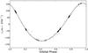 |
Fig. 1 Radial velocity curve of HD 217107 vs. orbital phase. The crosses mark the observations of Wittenmyer et al. (2007), which we used to compute this orbital solution. The boxes over the curve indicate the coverage of our observations, the filled boxes represent the runs utilized in the analysis, while the open boxes represent the discarded runs (details in Sect. 4.2). |
2.3. Flux estimate
By simulating the spectra of the planet and its host star as black bodies, we can estimate the order of magnitude of the planet-to-star flux ratio as a function of wavelength. The black body emission, Fλ(T), is determined by the surface temperature of the object. While for the star the temperature is well known from models (see Table 1), for the planet our best approximation is the equilibrium temperature  (2)For a reference value of the bond albedo of A = 0, we found an equilibrium temperature for HD 217107 b of Teq = 1040 ± 19 K. Figure 2 shows the black body spectrum of the star and the planet assuming a radius between one and two Jupiter radii, which is the range of the radii for giant extrasolar planets measured to date.
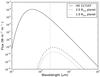 |
Fig. 2 Black body emission of HD 217107 and HD 217107 b assuming a planet radius of 1.0 and 2.0 Jupiter radii. The vertical dashed line marks the waveband of our data (2.14 μm). The directly reflected light component has little contribution in the infrared and is thus omitted. |
The planet-to-star flux ratio is given by 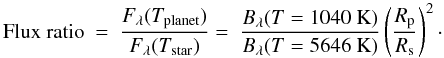 (3)At 2.14 μm, the flux ratio varies between 3 × 10⁻⁵ and 1.5 × 10⁻⁴ from one to two Jupiter radii of the planet’s radii, respectively. For shorter wavelengths the flux ratio decreases, because the star light dominates the emission spectrum. For longer wavelengths the net fluxes and thus the signal to noise ratio are lower.
3. Observations and data reduction
3.1. Observations
We observed the planetary system HD 217107 in 11 nights between 2007 August 14 and November 28 using Phoenix (Hinkle et al. 2003), a high-resolution near-infrared spectrometer at the Gemini South Observatory.
The spectrograph has a 256 × 1024 InSb Aladdin II array with a resolving power of μm per pixel, the slit covers 14 arcsec in length. Its gain is 9.2 e−/ADU and it has a readout noise of 40 electrons. An argon hollow cathode wavelength calibration source is supplied with the instrument. Over 950 frames of the system were obtained in service mode, using the standard ABBA nodding sequences to easily remove sky emission, they cover a portion in the infrared spectral range from 2.136 to 2.145 μm (see Table 2). We tuned the data acquisition after receiving the data from the first runs since the instrument was not fully characterized for use on the Gemini Telescope. For the first two nights, the exposure time was set to 25 s, whereas for the rest of the nights it was set to 80 s. We requested arc-lamp calibration exposures as well.
Phoenix observations of HD 217107.
3.2. Reduction
We wrote our own interactive data language (IDL)2 routines for the data reduction and analysis, processing each night and slit position as an independent data set to minimize systematics caused by different atmospheric conditions or instrumental set-up. We used the flat-field images to identify hot pixels, marking a pixel as bad if it had a value beyond 3.5 sigma from the median of the values of the nine subsequent pixels in its neighborhood. Bad pixels were masked in all further processing stages. Then, we divided the frames by a per-night master flat-field and subtracted their corresponding opposite A or B frame to remove bias and sky. Finally, we extracted the spectra from the frames with an IDL implementation3 of the optimal spectrum extraction algorithm described in Horne (1986), this algorithm identified cosmic ray hits, which were also masked from subsequent processing.
3.3. Wavelength calibration
First, we calibrated the wavelength dispersion using the ThAr lamps, identifying the line positions and strengths in a high-resolution ThAr line atlas (Hinkle et al. 2001). Because there was only one calibration lamp for each night, this solution represented only a rough wavelength calibration, because there are (sub pixel) offsets in wavelength in the data. To reach the high precision needed for this work, we fine-tuned the calibration with a high-resolution spectrum of the Sun4 to identify the telluric lines (identified as those present both in the solar spectrum and in an average spectrum of our data set).
We constructed an average spectrum to increase the S/N ratio by aligning and adding the spectra of each night. To determine the relative shifts, we selected within each set the first spectrum as reference, while the rest were shifted (using spline interpolations) to calculate the shift that minimized the root-mean-square of the correlation with the reference. The centers of fifteen common absorption lines were identified in wavelength values for the solar spectrum and in pixel position for our average spectrum. The wavelength solution is obtained by fitting a second-order polynomial (λ = c0 + c1p + c2p2) to the solar wavelength vs. the pixel position. Typical fitting coefficients are c0 = 2.145407, c1 = −1.0305 × 10⁻⁵, and c2 = −1.8496 × 10⁻¹⁰. The dispersion of the residuals is rms = 4.21 × 10⁻⁶μm. No pattern is seen in the residuals. Pixels at wavelengths dominated by the identified telluric absorption lines were discarded from subsequent processing owing to their highly variable nature. About 65% of the pixels remained for the next analysis steps.
4. Data analysis and results
4.1. Correlation
Because it is impossible to directly distinguish the planet’s signature from the stellar one in a single spectrum, following the idea of Deming et al. (2000) and Wiedemann et al. (2001), we searched for the planetary Doppler-shift signature through a correlation method between the (stellar-subtracted) residual data and a synthetic model of the planet’s spectrum. To remove the stellar flux, we aligned the spectra for each set (Doppler-shifting them and using a spline interpolation) in a reference system in which the star remains at rest, and constructed a stellar template from the average of the set. Then, the stellar templates and the spectra are normalized dividing by their respective medians. Finally, the wavelengths of the stellar templates are shifted according to the orbital phase of the star in each individual spectrum, and then the stellar template is subtracted from them. We avoided combining the different nights to obtain the stellar template, because it is highly probable that other systematics would be introduced.
Because the planet is approximately a thousand times less massive than its host star, the planetary Doppler wobble is greater by the same order of magnitude (see Eq. (1)), consequently the planetary signature will not be added coherently in the stellar template and thus appear blurred. The stellar template subtraction leaves a residual spectrum that consists of the signature of the planet, which is slightly attenuated in the averaging process and immersed in Poisson noise. The blurring of the planet signature (see Fig. 3) is determined by the planetary velocity span, which in turn depends on the time span of an observation and the orbital phase at the time of the observation. Observations near inferior or superior conjunction provide the greatest radial velocity spans, while observations close to the greater elongation of the planet’s orbit produce the smallest radial velocity spans, rendering the data useless. The rejected data sets in Table 2 were observed near greater elongation.
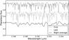 |
Fig. 3 Planetary spectrum blurring in the stellar template. Using our synthetic spectra of HD 217107 b we simulated the smearing of the planetary spectrum over one observing run. The dark-gray and light-gray lines denote the first and last spectra of HD 217107 b during an observing night. The relative shift owing to the orbital motion of HD 217107 b is 40 km s-1 in this simulation. The bottom black line shows averaged the planetary spectra. |
For the high-resolution synthetic planetary spectra of HD 217107 b we used customized theoretical thermal emission models of its atmosphere (model described in Fortney et al. 2005, 2006, 2008) at three different distances from the star to account for the non-negligible eccentricity of the planet. The models are cloud-free, with solar metallicity, gravity g = 20 m s-2, and the molecular abundances are those appropriate for chemical equilibrium. At these effective temperatures, the main absorbing molecules are H2O, CH4, CO, and CO2. The chemistry is described in detail in Lodders & Fegley (2002) and Visscher et al. (2006). We empirically characterized the instrumental resolution through the analysis of the emission lines in the calibration lamps. We convolved the model spectra by the instrumental resolution, which we determined to be . Then, for an assumed value of sini, the synthetic spectra are Doppler-shifted to mimic the radial velocity of the planet at the time that the data frame was obtained. The correlation degree, C(i), is calculated according to the formula 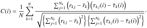 (4)In this equation we used the notation fkj for the value of the function at the pixel j of the spectrum k, and
  for the mean value of the function in the spectrum k. Here, “r” refers to the residual spectrum while “τ(i)” to the shifted planetary model spectrum, with Nk the number of pixels in spectrum k and N the total number of spectra. The denominator in the expression normalizes the correlation, and thus a value of 1.0 would indicate a perfect correlation.
We thus produce a curve of the correlation degree vs. the inclination of the orbit, evaluated in the range 0 < i < π/2. A positive value of this function indicates that the data spectrum resembles that of the model, while a negative one suggests anti-correlation. As consequence of the random nature of the Poisson noise, the value of the correlation between the residual spectra and the models should be close to zero, except when the adopted i matches that of the planetary system. Therefore, an appreciable peak in the correlation curve would represent a successful detection of the planetary signature and immediately indicates the value of i. By constraining the inclination with this method, the mass of the planet would be immediately determined via Eq. (1).
4.2. Data results
For this analysis, we excluded the nights where the velocity span of the star was less than 10 m s-1 (Col. 4 of Table 2) since they do not represent any significant improvement in the results, because the shift of the planet (~8.3 km s-1) is not significantly higher than the instrumental resolution (~7.5 km s-1). Figure 4 (Top panel) shows the correlation curve derived from our data as a function of sini. The degree of correlation found was close to zero at all inclinations, and we do not distinguish any identifiable positive peak that could indicate an atmosphere with absorption features resembling those of the models.
4.3. Planet-to-star flux ratio fitting
While the inclination determines the maximum of the correlation curve, the planet-to-star flux ratio () is the main physical parameter bounded to the magnitude of the correlation. In this section we determine the most probable values in the parameter space [ , sini], which gave rise to our result, and estimate the statistical significance of the value of the correlation reached. We searched for the best fitting values comparing our data results (Fig. 4 Top) with “synthetic” correlation curves. We generated the synthetic correlation curves by recreating our observations, adding a synthetic planetary spectrum, with known inclination and planet-to-star flux ratio, according to the following scheme: Step 1: we rearranged the order of the data set with random permutations within each night, but kept the original order of the dates of the observations. As a consequence, any real planet signature disappeared, but the noise level of the data was conserved. Step 2: using the atmospheric models of the planet, we injected a synthetic spectrum in the scrambled data set, Doppler-shifted and with a relative flux according to specific values of sini and , respectively. For simplicity, we adopted a constant along the orbit. Step 3: we processed these synthetic data through the same routines as in our original data (Sect. 4.1). We then iterated for a grid of values in the ranges: 0 ≤ i ≤ π/2 and 10-5 ≤ Fp/Fs ≤ 10-2, obtaining a set of synthetic correlations for sini and .
Once we obtained these models, we searched for the best-fit parameters through a χ2 minimization between the data correlation curve and the synthetic correlation curves, generating a goodness-of-fit map (Fig. 4, bottom panel).
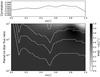 |
Fig. 4 Top: correlation result for our data set as a function of sini. The correlation remains flat along every inclination without any distinctive peak, the maximum value is reached at sini = 0.71. Bottom: goodness of fit, χ2-map, of the correlation models to the data. The horizontal and vertical axes refer to the fitting parameters sini and Fp/Fs respectively, at which the synthetic planetary spectrum was added in the correlation models creation, from which we calculated the minimum squares ( |


In addition, we used a bootstrap procedure to calculate false-alarm-probability limits for this map. Following Collier Cameron et al. (2002), we determined the frequency with which the correlation degree exceeds a given value as a result of noise in the absence of a planet signal. The routine consists of performing a random permutation of the data sets and the subsequent data analysis (steps 1 and 3 of previous paragraphs) which we repeated with a large number of times (~5000), recording the correlation curve after each trial. This set of correlation curves represents the correlation found in the absence of a planetary signal, and, because it is created from the data themselves, defines an empirical probability distribution that includes both the photon statistics and instrumental systematics.
Then, at each inclination, we stacked and sorted the values of the correlation in increasing order. We determined the 1, 2, 3, and 4-σ false-alarm confidence levels as the value of the correlation degree at the 65, 90, 99 and 99.9 percentiles of the trials. They represent the signal strengths at which spurious detections occur with 35, 10, 1, and 0.1 percent false-alarm probability respectively, at each value of the inclination. This allows us to assess the probability of obtaining a certain correlation degree in the absence of planetary emission.
Figure 4 (Bottom panel) shows the probability map for HD 217107 b. The best fit occurs at sini = 0.838 and Fp/Fs = 3.6 × 10⁻³, although the relative improvement in χ2 against the surrounding parameters is shallow. This value disagrees with the maximum value of the correlation curve (Fig. 4 Top), and furthermore, the bootstrap results indicate that this value is below the 3-σ confidence limit of the signal not being a false positive. Also, this is much higher than the predicted value from Sect. 2.3 (between 3 × 10⁻⁵ and 1.5 × 10⁻⁴). The disagreement of the results of the top and bottom panel in Fig. 4 suggests that systematics remain after the data reduction, while the strength of the correlation value, two orders of magnitude above the expected flux ratio, indicates that this result is not realistic. The 3-σ confidence limit only allows us to establish an upper limit in the flux ratio at 4–5 × 10⁻³ for inclinations greater than sini = 0.6. In conclusion, we cannot state the detection of HD 217107 b.
5. Future prospects
5.1. Observational strategy
Although our current data do not enable us to claim the detection of HD 217107 b, we identified a strategy to maximize the chances of a successful detection. This involves selecting suitable candidate systems and precisely choosing the phasing and span of the observations. To exemplify the advantages, we simulated realistic observations of other planetary systems.
We limited our sample to the currently known extrasolar planets without transits5, observables from Gemini South, for the first semester of the year. Even though we constrained ourselves to the instrument we characterized and to a fixed time span, the purpose of these simulations is to provide one successful detection with our method. It is plausible that considering the full extent of possibilities, stronger signals can be acquired. The improvement in a detection, limited by purely photon noise, can be quantified by the planet-to-star flux ratio and the stellar flux, according to the expression (fluxes in number of photons)  (5)Then, for example, the spectrometer CRIRES with four times the wavelength coverage of that of Phoenix, has twice the sensitivity of Phoenix. We decided to simulate the Phoenix instrument, since it is well characterized by our group, while other instruments should present their own systematics, which are hard to quantify.
We simulated the planets as if the strength of the high-resolution absorption features were the same as that of our models for HD 217107 b, but with the corresponding (estimated as in Sect. 2.3). A caveat for this assumption is that the strength of the lines is not very clear in planets that exhibit thermal inversions. Burrows et al. (2008) and Fortney et al. (2008) suggest that the emission features should be weaker.
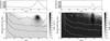 |
Fig. 5 Correlation curves and χ2-maps of synthetic data of HD 179949. A synthetic planetary signal was injected in the spectra with parameters: sini = 0.77 and Fp/Fs = 0.003. Left: using our observing strategy. Right: random distributed observing dates. The routine successfully recovers the signal at sini = 0.78 and Fp/Fs = 2.8 × 10⁻³ in both cases, although, when using our strategy, the correlation degree is stronger, and the parameters are better determined compared with the right panel. |
The target selection criteria are based first on the radial velocity span of the planet, where we set a lower limit cutoff of 7.5 km s-1 (equivalent to the FWHM of the instrument spectral resolution) for a three-hour observing run if the orbit was at i = 30°. Second, we look for higher apparent brightnesses of the stars for better signal-to-noise ratios. Table 3 lists two of the better suited selected planetary systems (HD 217107 listed for comparison). A brighter K-band magnitude of the star improves the signal-to-noise ratio, while a smaller semi-major axis involves a higher radial velocity span, which enables a greater Doppler shift of the planet spectra during the runs and at the same time favors higher planet-to-star flux ratios.
Favorable targets for Gemini South.
To simulate the observations, we recreated the same instrumental settings of our data, but carefully selected the observing schedule. For each one of the nights in the period and restricted to air masses under 1.5, we selected the three-hour range that gives the maximum velocity span. We recorded then, the radial velocity spans for each night, and chose those with the biggest spans. We used the solar spectrum to simulate the stellar spectrum, while for the planetary component we used the atmospheric models of HD 217107 b added with a given planet-to-star flux ratio and inclination. Each component is Doppler-shifted according to the orbital parameters. Finally we added Poisson noise to the spectra, according to the signal-to-noise corresponding to the magnitude of the target. The synthetic data were processed in exactly the same way as our original data.
5.2. Simulations
In our first test, we present two simulations of an observing campaign on a target with the physical parameters of HD 179949 to show the improvements of our observing strategy in contrast with a regular observation. The given parameters are sini = 0.77 and Fp/Fs = 3 × 10⁻³. Figure 5 left shows the simulation following our observing strategy, while Fig. 5 right shows the simulation selecting random observing dates. In both cases the correlation curves (top panels) mark the inclination of the synthetic orbit with a increment in the correlation degree near sini = 0.77, while the χ2-maps (bottom panels) effectively indicate the best fit at sini = 0.78 and Fp/Fs = 2.8 × 10⁻³.
We identify the main differences between these two simulations: first, given the larger radial velocity spans when implementing our strategy, the planetary spectrum is more blurred in the stellar template and consequently less reduced when the template is subtracted, the planetary spectrum signal is thus stronger in the residual spectrum, which increases the correlation degree. As consequence of these greater correlation degrees, all confidence levels are generally lower, because it is less probable to reach this correlation degree by chance in the no-planet case, and lastly, the χ2-map peak is much better determined. The improvement is reflected more in the distinction of the best fit against other values of the parameter space than in the distinction against the no-planet case.
In another simulation, we recreated the planetary system Tau Boo as close as possible to its real physical characteristics (Fig. 6). Tau Boo b had the parameters sini = 0.82 and Fp/Fs = 4 × 10⁻⁴, our routines returned the best fit: sini = 0.79 and Fp/Fs = 3.6 × 10⁻⁴, slightly underestimating the values. Nevertheless, the χ2-map shows an improvement in the region near the injected inclination and flux ratio. The bootstrap results set the 3–σ confidence limit near Fp/Fs 1.5 × 10⁻⁴ (for sini > 0.5), indicating a detection with 99% confidence.
6. Discussion and conclusions
Because the instrument was not well characterized at the time and our service-mode observational strategy had to be adapted after the first few observing windows, the data for HD 217107 were not as sensitive as expected. The correlation curve was featureless for all inclinations and with values close to zero, with a maximum at sini = 0.71. By fitting the sine of the inclination and the planet-to-star flux ratio through least-squares, we found the best-fit parameters of sini = 0.84 and Fp/Fs = 3.6 × 10⁻³ at a level below our 3-σ confident limit. As a consequence of the faint features in the results, the disagreement between the peak in the correlation (Fig. 4 Top panel) and the most probable value of sini (Fig. 4 Bottom panel), and the higher than predicted Fp/Fs, we could not claim a detection of HD 217107 b with our current data. Given the results of the bootstrap procedure, we reject the flux ratio of HD 217107 b to its host star to be over 5 × 10⁻³ (3-σ confidence). We attribute these results to the absence of an ideal strategy in the data acquisition at the time of the observations and a needed further treatment of the instrument systematics.
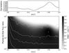 |
Fig. 6 Similar to Fig. 4, correlation curve (top panel) and χ2-map (bottom panel) of a simulation of the planetary system Tau Boo, with an injected companion at sini = 0.82 and Fp/Fs = 4 × 10⁻⁴. |
We could not detect HD 217107 b, but defined the outlines of future campaigns by carefully defining a candidate selection criterion and an observational strategy. We conclude that the best-suited candidates for this technique are those in very close orbits, which allow the planets to have high orbital velocities and higher planet-to-star flux ratios. We propose an observing strategy where for the period of observations we specifically select the nights with maximum radial velocity spans. To explore the capabilities of our routines, we simulated other planetary systems as observed by the Phoenix spectrograph, with the same number of hours and an appropriate schedule of observations. The system HD 179949 was recreated, contrasting the use of our observing strategy with a regular observation schedule. We recovered the planetary signature in both cases, but showing an improvement in the correlation degree, precision in the χ2-map, and lower σ limits when using our observing schedule. Finally, we performed a realistic simulation of the planetary system Tau Boo, and successfully detected its signature.
In conclusion high-resolution instruments like Phoenix are capable of detecting extrasolar planet Doppler-shifted signals with flux ratios as low as 104 with this method if we perform a careful treatment of the systematics (approaching the photon noise limit), if we count with appropriate theoretical models, and if we follow an optimized scheme in the data acquisition. Furthermore, using other instruments like CRIRES or NIRSPEC could increase the confidence of the results. Since our simulations exclude systematics effects specific to the instrument, an adequate treatment to remove them would be necessary. Our optimal observing strategy tends to select observations at superior conjunctions of the planet’s orbit, capturing the highest amount of light possible from the planet and at the same time covering the highest radial velocity span for a determined time extent. Refinements of this technique will involve the optimization of the distribution of time designated to the length of an observing run vs. the number of nights of observation, while adding phase-dependent functions of the planet’s brightness to account for the changing observed portion of the day/night side of the planet, and for different amounts of irradiation in eccentric orbits, will increase the accurateness of the fitted parameters.
Acknowledgments
Patricio Cubillos and Patricio Rojo are supported by the FONDAP Center for Astrophysics 15010003, the center of excellence in Astrophysics and Associated Technologies (PFB06) and the FONDECYT project 11080271.
References
- Barnes, J. R., Leigh, C. J., Jones, H. R. A., et al. 2007, MNRAS, 379, 1097 [NASA ADS] [CrossRef] [Google Scholar]
- Barnes, J. R., Barman, T. S., Jones, H. R. A., et al. 2008, MNRAS, 390, 1258 [NASA ADS] [CrossRef] [Google Scholar]
- Barnes, J. R., Barman, T. S., Jones, H. R. A., et al. 2010, MNRAS, 401, 445 [NASA ADS] [CrossRef] [Google Scholar]
- Burrows, A., Budaj, J., & Hubeny, I. 2008, ApJ, 678, 1436 [NASA ADS] [CrossRef] [Google Scholar]
- Butler, R. P., Wright, J. T., Marcy, G. W., et al. 2006, ApJ, 646, 505 [NASA ADS] [CrossRef] [Google Scholar]
- Cameron, A. C., Horne, K., Penny, A., & James, D. 1999, Nature, 402, 751 [NASA ADS] [CrossRef] [Google Scholar]
- Charbonneau, D., Brown, T. M., Latham, D. W., & Mayor, M. 2000, ApJ, 529, L45 [NASA ADS] [CrossRef] [PubMed] [Google Scholar]
- Collier Cameron, A., Horne, K., Penny, A., & Leigh, C. 2002, MNRAS, 330, 187 [NASA ADS] [CrossRef] [Google Scholar]
- Cutri, R. M., Skrutskie, M. F., van Dyk, S., et al. 2003, 2MASS All Sky Catalog of point sources [Google Scholar]
- Deming, D., Wiedemann, G., & Bjoraker, G. 2000, in From Giant Planets to Cool Stars, ed. C. A. Griffith, & M. S. Marley, ASP Conf. Ser., 212, 308 [Google Scholar]
- Fischer, D. A., Marcy, G. W., Butler, R. P., Vogt, S. S., & Apps, K. 1999, PASP, 111, 50 [NASA ADS] [CrossRef] [Google Scholar]
- Fischer, D. A., Marcy, G. W., Butler, R. P., et al. 2001, ApJ, 551, 1107 [NASA ADS] [CrossRef] [Google Scholar]
- Fortney, J. J., Marley, M. S., Lodders, K., Saumon, D., & Freedman, R. 2005, ApJ, 627, L69 [NASA ADS] [CrossRef] [Google Scholar]
- Fortney, J. J., Saumon, D., Marley, M. S., Lodders, K., & Freedman, R. S. 2006, ApJ, 642, 495 [NASA ADS] [CrossRef] [Google Scholar]
- Fortney, J. J., Lodders, K., Marley, M. S., & Freedman, R. S. 2008, ApJ, 678, 1419 [NASA ADS] [CrossRef] [Google Scholar]
- Henry, G. W., Marcy, G. W., Butler, R. P., & Vogt, S. S. 2000, ApJ, 529, L41 [NASA ADS] [CrossRef] [PubMed] [Google Scholar]
- Hinkle, K. H., Joyce, R. R., Hedden, A., Wallace, L., & Engleman, R. J. 2001, PASP, 113, 548 [NASA ADS] [CrossRef] [Google Scholar]
- Hinkle, K. H., Blum, R. D., Joyce, R. R., et al. 2003, in SPIE Conf., ed. P. Guhathakurta, 4834, 353 [Google Scholar]
- Horne, K. 1986, PASP, 98, 609 [NASA ADS] [CrossRef] [EDP Sciences] [Google Scholar]
- Knutson, H. A., Charbonneau, D., Allen, L. E., et al. 2007, Nature, 447, 183 [NASA ADS] [CrossRef] [PubMed] [Google Scholar]
- Knutson, H. A., Charbonneau, D., Allen, L. E., Burrows, A., & Megeath, S. T. 2008, ApJ, 673, 526 [NASA ADS] [CrossRef] [Google Scholar]
- Lodders, K., & Fegley, B. 2002, Icarus, 155, 393 [NASA ADS] [CrossRef] [Google Scholar]
- Lucas, P. W., & Roche, P. F. 2002, MNRAS, 336, 637 [NASA ADS] [CrossRef] [Google Scholar]
- Naef, D., Mayor, M., Pepe, F., et al. 2001, A&A, 375, 205 [NASA ADS] [CrossRef] [EDP Sciences] [Google Scholar]
- Perryman, M. A. C., & ESA 1997, The HIPPARCOS and TYCHO catalogues. Astrometric and photometric star catalogues derived from the ESA HIPPARCOS Space Astrometry Mission ESA Special Publication, 1200 [Google Scholar]
- Rodler, F., Kürster, M., & Henning, T. 2008, A&A, 485, 859 [NASA ADS] [CrossRef] [EDP Sciences] [Google Scholar]
- Rodler, F., Kürster, M., & Henning, T. 2010, A&A, 514, A23 [NASA ADS] [CrossRef] [EDP Sciences] [Google Scholar]
- Santos, N. C., Israelian, G., & Mayor, M. 2004, A&A, 415, 1153 [NASA ADS] [CrossRef] [EDP Sciences] [Google Scholar]
- Snellen, I. A. G., de Kok, R. J., de Mooij, E. J. W., & Albrecht, S. 2010, Nature, 465, 1049 [NASA ADS] [CrossRef] [PubMed] [Google Scholar]
- Swain, M. R., Vasisht, G., & Tinetti, G. 2008, Nature, 452, 329 [NASA ADS] [CrossRef] [PubMed] [Google Scholar]
- Tinetti, G., Vidal-Madjar, A., Liang, M.-C., et al. 2007, Nature, 448, 169 [NASA ADS] [CrossRef] [PubMed] [Google Scholar]
- Visscher, C., Lodders, K., & Fegley, Jr., B. 2006, ApJ, 648, 1181 [NASA ADS] [CrossRef] [Google Scholar]
- Vogt, S. S., Butler, R. P., Marcy, G. W., et al. 2005, ApJ, 632, 638 [NASA ADS] [CrossRef] [Google Scholar]
- Wiedemann, G., Deming, D., & Bjoraker, G. 2001, ApJ, 546, 1068 [NASA ADS] [CrossRef] [Google Scholar]
- Wittenmyer, R. A., Endl, M., & Cochran, W. D. 2007, ApJ, 654, 625 [NASA ADS] [CrossRef] [Google Scholar]
- Wright, J. T., Upadhyay, S., Marcy, G. W., et al. 2009, ApJ, 693, 1084 [NASA ADS] [CrossRef] [Google Scholar]
All Tables
All Figures
|
Fig. 1 Radial velocity curve of HD 217107 vs. orbital phase. The crosses mark the observations of Wittenmyer et al. (2007), which we used to compute this orbital solution. The boxes over the curve indicate the coverage of our observations, the filled boxes represent the runs utilized in the analysis, while the open boxes represent the discarded runs (details in Sect. 4.2). |
| In the text | |
|
Fig. 2 Black body emission of HD 217107 and HD 217107 b assuming a planet radius of 1.0 and 2.0 Jupiter radii. The vertical dashed line marks the waveband of our data (2.14 μm). The directly reflected light component has little contribution in the infrared and is thus omitted. |
| In the text | |
|
Fig. 3 Planetary spectrum blurring in the stellar template. Using our synthetic spectra of HD 217107 b we simulated the smearing of the planetary spectrum over one observing run. The dark-gray and light-gray lines denote the first and last spectra of HD 217107 b during an observing night. The relative shift owing to the orbital motion of HD 217107 b is 40 km s-1 in this simulation. The bottom black line shows averaged the planetary spectra. |
| In the text | |
|
Fig. 4 Top: correlation result for our data set as a function of sini. The correlation remains flat along every inclination without any distinctive peak, the maximum value is reached at sini = 0.71. Bottom: goodness of fit, χ2-map, of the correlation models to the data. The horizontal and vertical axes refer to the fitting parameters sini and Fp/Fs respectively, at which the synthetic planetary spectrum was added in the correlation models creation, from which we calculated the minimum squares ( |
| In the text | |
|
Fig. 5 Correlation curves and χ2-maps of synthetic data of HD 179949. A synthetic planetary signal was injected in the spectra with parameters: sini = 0.77 and Fp/Fs = 0.003. Left: using our observing strategy. Right: random distributed observing dates. The routine successfully recovers the signal at sini = 0.78 and Fp/Fs = 2.8 × 10⁻³ in both cases, although, when using our strategy, the correlation degree is stronger, and the parameters are better determined compared with the right panel. |
| In the text | |
|
Fig. 6 Similar to Fig. 4, correlation curve (top panel) and χ2-map (bottom panel) of a simulation of the planetary system Tau Boo, with an injected companion at sini = 0.82 and Fp/Fs = 4 × 10⁻⁴. |
| In the text | |
Current usage metrics show cumulative count of Article Views (full-text article views including HTML views, PDF and ePub downloads, according to the available data) and Abstracts Views on Vision4Press platform.
Data correspond to usage on the plateform after 2015. The current usage metrics is available 48-96 hours after online publication and is updated daily on week days.
Initial download of the metrics may take a while.