| Issue |
A&A
Volume 528, April 2011
|
|
|---|---|---|
| Article Number | A42 | |
| Number of page(s) | 8 | |
| Section | Extragalactic astronomy | |
| DOI | https://doi.org/10.1051/0004-6361/201016188 | |
| Published online | 25 February 2011 | |
Flux and color variations of the quadruply imaged quasar HE 0435-1223⋆
1 Département d’Astrophysique, Géophysique et Océanographie,
Bât. B5C, Sart Tilman, Université de Liège, 4000 Liège 1, Belgique
e-mail: ricci@astro.ulg.ac.be
2
Main Astronomical Observatory, Academy of Sciences of Ukraine,
Zabolotnoho 27,
03680
Kyiv,
Ukraine
3
Centro de Astro-Ingeniería, Departamento de Astronomía y
Astrofísica, Pontificia Universidad Católica de Chile, Casilla 306, Santiago, Chile
4
Max-Planck-Institut für Astronomie, Königstuhl 17, 69117
Heidelberg,
Germany
5 Dipartimento di Fisica “E.R. Caianiello”, Università degli
Studi di Salerno, via Ponte Don Melillo, 84085 Fisciano (SA), Italy
6
Instituto Nazionale di Fisica Nucleare,
Sezione di Napoli,
Italy
7
SUPA, University of St Andrews, School of Physics &
Astronomy, North
Haugh, St Andrews,
KY16 9SS,
UK
8
Deutsches SOFIA Institut, Universitaet Stuttgart,
Pfaffenwaldring 31,
70569
Stuttgart,
Germany
9 Istituto Internazionale per gli Alti Studi Scientifici
(IIASS), Vietri Sul Mare (SA), Italy
10
Institut für Astrophysik, Georg-August-Universität Göttingen,
Friedrich-Hund-Platz
1, 37077
Göttingen,
Germany
11
Department of Physics & Astronomy, Aarhus
University, Ny
Munkegade, 8000
Aarhus C,
Denmark
12
Niels Bohr Institute, University of Copenhagen,
Juliane Maries vej
30, 2100
Copenhagen Ø,
Denmark
13
KASI – Korea Astronomy and Space Science Institute,
61-1 Hwaam-dong,
Yuseong-gu, Daejeon
305-348, Republic of
Korea
14
National Space Institute, Technical University of Denmark,
2800
Lyngby,
Denmark
15
Astronomisches Rechen-Institut, Zentrum für Astronomie,
Universität Heidelberg, Mönchhofstraße 12-14, 69120
Heidelberg,
Germany
16
Dipartimento di Ingegneria, Università del Sannio,
Corso Garibaldi 107,
82100
Benevento,
Italy
17 Bellatrix Astronomical Observatory, Center for Backyard
Astrophysics, Ceccano (FR), Italy
18
Physics Department, Sharif University of Technology,
Tehran,
Iran
19
European Southern Observatory, Casilla 19001, Santiago 19, Chile
20
Max Planck Institute for Solar System Research,
Max-Planck-Str. 2,
37191
Katlenburg-Lindau,
Germany
21
Astrophysics Group, Keele University, Newcastle-under Lyme, ST5 5BG, UK
22
Dark Cosmology Centre, Niels Bohr Institute, University of
Copenhagen, Juliane Maries Vej
30, 2100
Copenhagen,
Denmark
23
INAF – Osservatorio Astronomico di Brera,
23807
Merate,
Italy
24
SOFIA Science Center, NASA Ames Research Center, Mail Stop N211-3,
Moffett Field
CA
94035,
USA
25
Centre for Star and Planet Formation, Geological Museum, Øster
Voldgade 5, 1350
Copenhagen,
Denmark
Received: 23 November 2010
Accepted: 10 January 2011
Aims. We present VRi photometric observations of the quadruply imaged quasarHE0435-1223, carried out with the Danish 1.54 m telescope at the La Silla Observatory. Our aim was to monitor and study the magnitudes and colors of each lensed component as a function of time.
Methods. We monitored the object during two seasons (2008 and 2009) in the VRi spectral bands, and reduced the data with two independent techniques: difference imaging and point spread function (PSF) fitting.
Results. Between these two seasons, our results show an evident decrease in flux by ≈ 0.2–0.4 magnitudes of the four lensed components in the three filters. We also found a significant increase ( ≈ 0.05–0.015) in their V − R and R − i color indices.
Conclusions. These flux and color variations are very likely caused by intrinsic variations of the quasar between the observed epochs. Microlensing effects probably also affect the brightest “A” lensed component.
Key words: quasars: general / gravitational lensing: weak / techniques: photometric
Based on data collected by MiNDSTEp with the Danish 1.54 m telescope at the ESO La Silla Observatory. Tables 5–7 are only available in electronic form at the CDS via anonymous ftp to cdsarc.u-strasbg.fr (130.79.128.5) or via http://cdsarc.u-strasbg.fr/viz-bin/qcat?J/A+A/528/A42
© ESO, 2011
1. Introduction
In the framework of the MiNDSTEp (Microlensing Network for the Detection of Small Terrestrial Exoplanets) campaign (Dominik et al. 2010), which has as a main target the systematic observation of bulge microlenses, we developed a parallel project concerning photometric multi-band observations of several lensed quasars1. In the present paper we focus on HE0435-1223 (see Fig. 1), a QSO discovered by Wisotzki et al. (2000) in the course of the Hamburg/ESO digital objective prism survey, and confirmed to be a quadruply imaged quasar by Wisotzki et al. (2002). The lensing galaxy was initially identified as an elliptical with a scale length of ≈ 12 kpc at a redshift in the range z = 0.3–0.4. The time delays between the four images (labeled “A”, “B”, “C”, “D”, starting from the brighter one and proceeding clockwise) of the quasar were estimated around 10 days, and the quasar itself showed some signs of intrinsic variability (Wisotzki et al. 2002).
More recently, the value of the redshift for the lensing galaxy was estimated as z = 0.44 ± 0.20, and the quasar redshift was confirmed to be z = 1.6895 ± 0.0005, with a Δz between the components of ≈ 0.0015 rms (Wisotzki et al. 2003). These spectrophotomeric observations showed some possible signature of microlensing effects in the continuum and in the spectral emission lines for the “D” component.
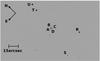 |
Fig. 1 Zoom of a DFOSC i filter image showing the four components of the lensed quasar and four nearby stars. The components are labeled following the notation of Wisotzki et al. (2002): “A” for the brighter component, “B”, “C” and“D” clockwise. The stars “R”, “S”, “T” and “U” were used to search for a suitable reference star. The “R” star was finally chosen. The contrast of the displayed image, on a negative scale, was selected to improve the visibility of the lensed components. The image is a median of the three CCD frames collected on 2008 August 8. |
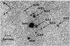 |
Fig. 2 Zoom of a DFOSC i filter image showing the galaxy environment near HE0435-1223. The objects are labeled following the notation of Morgan et al. (2005). The contrast, on a negative scale, was selected to improve the visibility of the galaxies. The image is a median of the three CCD frames collected on 2008 August 8. |
Morgan et al. (2005) provided milliarcsecond astrometry, revised the value of the lens redshift at z = 0.4546 ± 0.0002 with the Low-Dispersion Survey Spectrograph 2 (LDSS2) on the Clay 6.5 m telescope, and studied the galaxy environment of the lens, because it is located in a dense galaxy field. The results do not show any evidence of a cluster for the considered galaxies. However, the nearest galaxies (G20, G21, G22, G23, and G24 in Fig. 2) whose redshifts were not measured, left this scenario open. Nevertheless, the results of a deep investigation concerning the direction of an external shear in the gravitational field of the lens do not show an evident correlation with the position of the near galaxies. As a remaining explanation, Morgan et al. (2005) suggested the presence of substructures in the lensing galaxy.
The first systematic monitoring, which was performed in the R filter and covered the years between 2003 and 2005, was carried out by Kochanek et al. (2006): that paper provided astrometric measurements compatible with the previous works, measured the time delays between the images (ΔtAD = −14.37, ΔtAB = −8.00, and ΔtAC = −2.10 days, with errors respectively of 6%, 10% and 35%), and finally confirmed the lensing galaxy as an elliptical with a rising rotation curve.
Furthermore, Mediavilla et al. (2009) observed HE0435-1223 in the framework of a monitoring of 29 lensed quasars, and attributed eventual microlensing events to the normal stellar populations, while Blackburne & Kochanek (2010) focused on the quasar itself, applying a model with a time-variable accretion disk to the object. Mosquera et al. (2011) found clear evidence of chromatic microlensing in the “A” component, and provided an estimate of the disk size in the R band in agreement with the simple thin-disk model. Blackburne et al. (2011) used the chromatic microlensing to model the accretion disk, and Courbin et al. (2010) recalculated the time delays with N-body realizations of the lensing galaxy, which he thought to belong to the “B component” (ΔtBA = 8.4, ΔtBC = 7.8 and days with errors of 25%, 10%, and 11% respectively). Considering multi-color observations of other lensed quasars, a single-epoch multi-band photometry was used on MG0414+0534 to constrain the accretion disk model and the size of the emission region in the continuum (Bate et al. 2008; Bate 2008; Floyd et al. 2008).
A multi-epoch multi-band photometry, carried out during several years, was used for the quasar Q2237+0305 by Koptelova et al. (2006), who observed the object during five years (1995–2000) in the VRI bands. Anguita et al. (2008) combined these data with OGLE observations. Mosquera et al. (2009) monitored the object in eight filters and found evidence for microlensing in the continuum, but not in the emission lines. Furthermore, Q2237+0305 was the object of deep studies focused on the lens galaxy (Poindexter & Kochanek 2010b), and on the inclination of the accretion disk (Poindexter & Kochanek 2010a). Another example of multi-epoch multi-band observations is given by UM673/Q0142–100, observed in the Gunn i and Cousins V filters between 1998 and 1999 (Nakos et al. 2005) and in the VRI bands between 2003 and 2005 (Koptelova et al. 2010). Unlike for these objects, no systematic multi-band photometry has ever been carried out for HE0435-1223.
Here, we present two periods of multi-band photometric observations of HE0435-1223, performed in the VRi spectral bands with the Danish 1.54 m telescope at the La Silla Observatory.
In Sect. 2 we explain how the observations were carried out; in Sect. 3 we focus on the data reduction, and we describe the two independent techniques: difference imaging and point spread function (PSF) fitting, that were used to construct the light curves. In Sect. 4 we present the results. Finally, in Sect. 5 we summarize the conclusions.
2. Observations and pre-processing
We observed HE0435-1223 during two seasons (2008 and 2009) with the Danish 1.54m telescope at the La Silla Observatory. We used the DFOSC instrument (Danish Faint Object Spectrograph and Camera) for imaging and photometry, with a 2147 × 2101 CCD device, covering a 13.7′ × 13.7′ field of view with a resolution of 0.39″/pixel. The gain of the device is 0.74 electron/ADU in high mode, while the read out noise in this mode is 3.1 electrons (Sørensen 2000).
The data were collected in three different filters: Gunn i, Bessel R and Bessel V (see Table 1 and Fig. 3). We worked with a very homogeneous dataset consisting of 180s exposures.
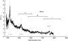 |
Fig. 3 Position and bandwidth of the VRi DFOSC filters superposed on the unresolved spectrum of HE0435-1223. The figure is a composition made from the spectrum shown in the paper of Wisotzki et al. (2002). |
For almost every night of observation, we also collected bias images and dome flat-fields, which were already treated in loco using an automatic IDL procedure, part of the MiNDSTEp pipeline for the observation of bulge microlenses. We then obtained master flat-fields for the different filters and master biases. When these images were not present for the desired date, we coupled the most recent set of master bias and master flat-fields to our science dataset, in the phase of pre-processing.
We collected a total of 391 images during the 2008 season, and 160 images in 2009.
The images were pre-processed (de-biased and flat-fielded), and we used particularly the dome flats. To erase the possible residual halos caused by the inhomogeneous illumination, the sky background was subtracted fitting a 4th degree surface after masking the stars and cosmic rays, and the images were recentered with an accuracy of 1 px.
These steps were performed with a C++ pipeline developed by our team.
We analyzed each image to sort out and then disregard the problematic images in terms of bad tracking, particularly bad seeing (the components were completely unresolved) or bad focusing.
We then obtained 216 images during the 2008 season: 70 in the i filter, covering 26 nights, 83 in the R filter, covering 32 nights, and 63 in the V filter, covering 25 nights, distributed between 2008 July 27 and 2008 October 4.
Concerning the 2009 season, we obtained 116 images: 46 in the i filter, covering 17 nights, 37 in the R filter, covering 14 nights, and 33 in the V filter, covering 12 nights, distributed between 2009 August 20 and 2009 September 19.
3. Data reduction
As a first step, we chose four stars near HE0435-1223, labeled “R”, “S”, “T” and “U” in Fig. 1, to search for a stable reference star. We examined the ratios between the fluxes of these stars in the V band as a function of time, to possibly detect some photometric variations between the two seasons.
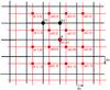 |
Fig. 4 Scheme for the superposed images of the first (little dots, lighter grid) and second (big dots, bolder grid) stars. The big dots correspond to the knots with known fluxes. The arrows Δx and Δy indicate the shift between the two images. |
For the calculation of the ratio between the fluxes of two selected stars we applied the PSF fitting method that was also subsequently used on the gravitational lens system itself. While using this method, we superposed the image of the first star over the fixed image of the second star as shown in Fig. 4. The red and black grids represent the images of the first and the second star, respectively.
The big dots correspond to the knots for which the counts are known. The values p(x,y) and S correspond to the counts for each knot of the first and the second star, respectively. To perform a precise fitting we needed to superpose these images with an accuracy better than 1 pixel. When this was done, the knots of both images did not perfectly coincide with each other as shown in Fig. 4. Therefore we had to calculate intermediate values, for example p(x,y), which we could compare with the value S at the same point. For that we used bicubic interpolation (Press et al. 1992). The intermediate value p(x,y) is expressed by the polynomial  (1)To derive the values of the 16 coefficients ai,j we resolved this set of equations for 16 knots around the considered point p(x,y). They are shown as red dots in Fig. 4. With this coefficient matrix ai,j we could derive p(x,y) at any point. For the fitting of both images we minimized the quantity
  (2)which is the sum over all knots k of the first star image; A is the ratio between the total flux of the second and the first star, Δx and Δy are the relative shifts (fractions of a pixel) between the two superposed images. Before the first iteration, we set the three parameters A, Δx and Δy within reasonable ranges.
Average V magnitude differences between the two epochs for the four stars near HE0435-1223.
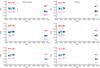 |
Fig. 5 Light curves of the four lensed components of HE0435-1223. The different graphs illustrate the photometry in the i, R and V bands, calculated using the difference imaging technique (left) and the PSF fitting technique (right). The error bars correspond to the magnitude rms (1σ) of each night of observation. |
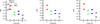 |
Fig. 6 Average magnitude of each component for the 2008 season (upper symbols) and 2009 (lower symbols), calculated with the difference imaging technique (left) and the PSF fitting method (right). The error bars correspond to the magnitude rms (1σ) during each epoch of observation. |
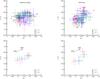 |
Fig. 7 Color-color diagrams for the four lensed components. The left column shows the V − R vs. R − i diagram calculated with the difference imaging technique: all observations (upper panel) and average of the observations for each season (lower panel). The right column shows the same diagrams calculated with the PSF fitting technique. |
VRi average magnitudes of the four lensed components of HE0435-1223 during the 2008 and 2009 seasons.
We derived the light curves for the reference stars as magnitude differences and calculated the average difference and standard deviations for the two epochs (see Table 2). Obviously the stellar pairs with the star “R” in Table 2 show on average the smallest differences between the two epochs. Moreover the light curves of the “R” star shows on average the least standard deviation σ (see Table 2), and we may reasonably assume that star “R” is the most stable reference star between the two seasons. Therefore we chose star “R” as the reference for all subsequent photometric zero point determinations.
The magnitude of the reference star was taken from the USNO-B1.0 catalog for the i and R filters (16.27 and 16.33 respectively), and from the NOMAD1 catalog for the V filter (17.04).
The light curves for the four components of the gravitational lens system were then calculated with two independent methods treated below: difference imaging and PSF fitting.
3.1. Difference imaging method
The aim of the difference imaging technique is to subtract from each image of our field (indicated as “frame” in the following) one image of the same field (called “reference frame”) taken at a different time under the best seeing conditions. This operation produces a set of subtracted frames where only the relative flux variations between the two images (generic frame and reference frame) are visible. Performing aperture photometry on these subtracted frames, and in particular at the positions of the lensed QSO components, we derived the light curves of the four lensed components.
However, differences in seeing, focus, and guiding precision between frames collected at different times may produce variations in the shape of the PSF: trying the subtraction without additional operations would produce high residuals caused by potential PSF slope variations. Several methods have been developed to force the PSF of the images to match (Alard 1999, 2000). These methods are particularly useful in crowded fields such as the galactic bulge, but are less succesful in sparse fields. In this paper we adopt the method proposed by Phillips (1993) which was already successfully applied by Nakos et al. (2005) and is based on FFT (Fast Fourier Transform).
If r is the reference frame and f a generic frame, then f = r ⊗ k, where k is the convolution kernel describing the differences between the PSF, which are unknown, and ⊗ indicates the convolution product. In the Fourier space, the previous equation can be noted as F = RK, where F, R and K represents the Fourier transform (F) of the generic frame f, the reference frame r, and the convolution kernel k. Then k = F-1(F/R).
Phillips (1993) considers the limits of this technique and the solutions adopted to avoid problems with background and high-frequency noise.
We normalized the frames in flux by fixing the magnitude of the reference star in each filter with the values of the catalogs mentioned above. Then we used the difference imaging method on the normalized frames. With this technique, all the not variable objects in the field disappear, which allows us automatically to suppress the contribution of the lensing galaxy, which is an extended and photometrically constant object.
To obtain the light curves, we performed aperture photometry of the residuals, using the positions of the selected reference star and of the lensed components previously derived. But we found for the 2009 images a weak linear dependence between the magnitude and the seeing, which we removed after calibrating this effect.
The procedure described in this paragraph is based on a code developed by our team, written in Python.
The results for the three filters are shown in the left column of Fig. 5. The error bars correspond to the magnitude rms (1σ) of each night of observation.
3.2. PSF fitting method
We also decided to calculate the light curves using PSF fitting as an independent method, which we previously employed to determine the most adequate reference star.
For the fitting of the lens system we used the image of star “R” as the PSF reference. Then we fitted each frame with five adjustable PSF for the four lensed quasar images and the lensing galaxy, taking the relative astrometric coordinates between the components from Kochanek et al. (2006). Note that the faint lensing galaxy is barely resolved on direct HST CCD frames (Morgan et al. 2005)3. Therefore, it is legitimate to model it with the PSF of our ground-based observations.
In this way we had seven free parameters: Δx, Δy (coordinates of the gravitational lens system with respect to the reference star “R”), and the central fluxes of the five components.
After minimization of the squared differences between the fluxes of the real lens system image and the simulated image with the five PSF, we derived the seven best-fitting parameters. We used bicubic interpolation for the superposition of the CCD frames to achieve results better than 1 pixel according to our description in Sect. 3. To construct the light curves, we calculated the flux ratios between each component and the reference star “R”. The procedure described in this paragraph is based on an Object Pascal code developed by our team.
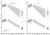 |
Fig. 8 Upper light curve: “global i” light curve of the four lensed components of HE0435-1223 obtained after subtracting the average 2008 i difference in magnitude from “B”, “C”, and “D” with respect to component “A”; then corrected for the time delays provided by Kochanek et al. (2006) and finally subtracting from the R and the V light curves the average 2008 R − i and (R − i) + (V − R) color indices, respectively. Lower light curve: “global i” light curve obtained repeating the same procedure as for the upper one, but correcting for the average 2008 magnitude and color indices concerning the 2008 data, and for the 2009 average magnitude and color indices concerning the 2009 data. The left panel shows the results obtained with the difference imaging technique, while the right panel shows the results obtained with the PSF fitting technique. The gray quadrilaterals help to connect the two epochs of observation. The lower light curves are arbitrarily shifted in magnitude. |
Averages and error bars (sigma) characterizing the V − R and R − i color indices of each component for the 2008 and 2009 seasons.
The results for the three filters are shown in the right column of Fig. 5. The error bars correspond to the magnitude rms (1σ) of each night of observation.
4. Results
Both methods show a significant decrease in flux of the four lensed components between the 2008 and 2009 seasons. The estimated amounts of the decrease are coherent between the two methods (see Fig. 6).
In order to estimate this decrease, we measured the mean and the σ for each component in each filter. The average values for the magnitudes and rms for each component, each filter and the 2008 and 2009 seasons, are reported in Table 3. Specifically, all the four components show a decrease by ≈ 0.2 − 0.4 magnitudes in each of the filters, although we notice a slightly larger amplitude for component “A” in the V band.
The corresponding values expressed in sigma units show a shift between ≈11.3σ and ≈13.7σ in the V band, except for component “A”, which shows a decrease by ≈ 26.3σ. In the R and i filters, the shift is between ≈6.5σ and 7.5σ, except for component “A” (≈15.0σ and ≈9.8σ respectively) and component “C” in the R band ( ≈ 12.0σ).
For the fraction of nights when the object was observed in all VRi filters, we were able to build the color-color diagram (V − R vs. R − i) for the four components. The results are shown in Fig. 7. With the same technique used to estimate the decrease in flux, we also found a significant increase (≈0.05–0.015) for the color indices V − R and R − i between the two observing seasons. The details are given in Table 4. In particular, component “A” shows the largest shift in color.
The corresponding values expressed in sigma units show a shift in color between ≈ 1.3σ and ≈ 2.0σ for the color indices V − R and R − i, except for component “A” (3.40σ in V − R and 3.1σ in R − i).
Given the short time delays (Kochanek et al. 2006) and because we expect microlensing to lead to uncorrelated flux variations between the four lensed components, these results support the assumption that the observed magnitude and color variations are very likely caused by intrinsic variations of the QSO, while the lensed “A” component is probably also affected by microlensing.
As a complementary approach, we decided to construct two “global i” light curves to better understand the nature of these different variations in flux and color index.
To construct the first one, we superposed the light curves of the four components by subtracting from “B”, “C”, and “D” their average 2008 difference in magnitude with respect to the “A” component, and we corrected the data for the time delays provided by Kochanek et al. (2006) (i.e, we applied to the components a shift in the MJD corresponding to the time delays). Then, we superposed the obtained curves (one for each filter) by subtracting from the R and the V light curves the average 2008 R − i and (R − i) + (V − R) color indices, respectively. The goal of this first “global i” light curve is to visualize how the spreads in magnitude and colors evolve between the epochs. The results are shown in Fig. 8 (upper light curves).
To construct the second “global i” light curve, we repeated the same procedure, but subtracted from the 2008 data of “B”, “C” and “D” the average 2008 difference in magnitude with respect to component “A”, and from 2009 data the corresponding average 2009 difference in magnitude. Similarly, we subtracted from the R and the V light curves the average 2008 and 2009 R − i and (R − i) + (V − R) color indices, respectively. The results are shown in Fig. 8 (lower curves).
After these superpositions, we observe in 2008 a scatter in the data (see Fig. 8) significantly larger than that of the individual light curves (see Fig. 5); and in general a difference in scatter between the two epochs that we attribute to intrinsic variations of the quasar both in magnitude and color.
We also observe a slight brightening of the lensed quasar in 2008, followed by a significant decrease in 2009. Our observations corroborate those recently reported by Courbin et al. (2010). Referring to the PSF-only fitting method, we were also able to estimate the magnitude of the lensing galaxy as 19.87 ± 0.10 in the i band; 20.47 ± 0.13 in the R band; and 21.89 ± 0.24 in the V band. Furthermore, no significant changes in the magnitude of the lensing galaxy were observed between the two epochs. Our results for the V and i filters are coherent with those of Wisotzki et al. (2002) and Morgan et al. (2005).
Proceeding in the same way, we did not find any evident color-shift for the lensing galaxy: we find a value of 1.47 ± 0.33 and 1.36 ± 0.21 for the V − R color index in 2008 and 2009, respectively; and 0.59 ± 0.17 and 0.61 ± 0.14 for the R − i color index.
The stability of the flux of the lensing galaxy over the two epochs enforces the validity of our PSF fitting software. We find that appreciably larger photometric error bars derived for the lensing galaxy are essentially caused by its faintness (V ≈ 21.9) compared with the four lensed components (V ∈ [18.4,19.5]).
5. Conclusion
Systematic multi-spectral band photometry of the quadruply imaged quasar HE0435-1223, carried out during two seasons (2008 and 2009), shows a significant decrease in flux of the four lensed components between the two epochs.
The drop in flux observed for the four lensed components between 2008 and 2009 is very likely caused by a change in the intrinsic luminosity of the quasar. This corroborates the previous studies of the HE0435-1223 gravitational lens system by Kochanek et al. (2006) and Courbin et al. (2010).
Concerning the color variations, the intrinsic reddening of a quasar when it becomes fainter in luminosity is an effect already observed in previous studies (Pereyra et al. 2006), and the same trend probably accounts for the similar observed changes in the colors of the four lensed components of HE0435-1223.
This hypothesis is enforced if we suppose that the intrinsic photometric quasar variations in the different colors are not synchronized, which provides an explanation for the differences in scatter between the epochs (see Fig. 8). Microlensing probably
provides the additional effect necessary to account for the higher flux variation observed for the “A” component.
The presented observations also show that a well sampled multi-band photometry can help in distinguishing the nature of the variability of multiply imaged objects, in particular gravitationally lensed quasars.
We suggest to couple this technique in the future with integral field spectroscopy to provide an additional way for an even more detailed investigation of the observed phenomena.
HE0435-1223, UM673/Q0142-100, Q2237+0305, WFI2033-4723 and HE0047-1756
Information available on the Internet at http://www.eso.org/lasilla/telescopes/d1p5/misc/dfosc_filters.html
Acknowledgments
The research was supported by ARC – Action de recherche concertée (Communauté Française de Belgique – Académie Wallonie-Europe). A.E. is the beneficiary of a fellowship granted by the Belgian Federal Science Policy Office. Astronomical research at Armagh Observatory is funded by the Department of Culture, Arts & Leisure (DCAL), Northern Ireland, UK. Operation of the Danish 1.54 m telescope is supported by the Danish National Science Research Council (FNU). We wish to thank the anonymous referee for the remarks and the suggestions.
References
- Alard, C. 1999 [arXiv:astro-ph/9903111] [Google Scholar]
- Alard, C. 2000, A&AS, 144, 363 [NASA ADS] [CrossRef] [EDP Sciences] [Google Scholar]
- Anguita, T., Schmidt, R. W., Turner, E. L., et al. 2008, A&A, 480, 327 [NASA ADS] [CrossRef] [EDP Sciences] [Google Scholar]
- Bate, N. 2008, in Manchester Microlensing Conference [Google Scholar]
- Bate, N. F., Floyd, D. J. E., Webster, R. L., & Wyithe, J. S. B. 2008, MNRAS, 391, 1955 [NASA ADS] [CrossRef] [Google Scholar]
- Blackburne, J. A., & Kochanek, C. S. 2010, ApJ, 718, 1079 [NASA ADS] [CrossRef] [Google Scholar]
- Blackburne, J. A., Pooley, D., Rappaport, S., & Schechter, P. L. 2011, ApJ, 729, 34 [NASA ADS] [CrossRef] [Google Scholar]
- Courbin, F., Chantry, V., Revaz, Y., et al. 2010, [arXiv:1009.1473] [Google Scholar]
- Dominik, M., Jørgensen, U. G., Rattenbury, N. J., et al. 2010, Astron. Nachr., 331, 671 [NASA ADS] [CrossRef] [Google Scholar]
- Floyd, D. J. E., Bate, N. F., & Webster, R. L. 2008, Mem. Soc. Astron. Ital., 79, 1271 [NASA ADS] [Google Scholar]
- Kochanek, C. S., Morgan, N. D., Falco, E. E., et al. 2006, ApJ, 640, 47 [NASA ADS] [CrossRef] [Google Scholar]
- Koptelova, E., Oknyanskij, V. L., Artamonov, B. P., & Burkhonov, O. 2010, MNRAS, 401, 2805 [NASA ADS] [CrossRef] [Google Scholar]
- Koptelova, E. A., Oknyanskij, V. L., & Shimanovskaya, E. V. 2006, A&A, 452, 37 [NASA ADS] [CrossRef] [EDP Sciences] [Google Scholar]
- Mediavilla, E., Muñoz, J. A., Falco, E., et al. 2009, ApJ, 706, 1451 [NASA ADS] [CrossRef] [Google Scholar]
- Morgan, N. D., Kochanek, C. S., Pevunova, O., & Schechter, P. L. 2005, AJ, 129, 2531 [NASA ADS] [CrossRef] [Google Scholar]
- Mosquera, A. M., Muñoz, J. A., & Mediavilla, E. 2009, ApJ, 691, 1292 [NASA ADS] [CrossRef] [Google Scholar]
- Mosquera, A. M., Muñoz, J. A., Mediavilla, E., & Kochanek, C. S. 2011, ApJ, 728, 145 [NASA ADS] [CrossRef] [Google Scholar]
- Nakos, T., Courbin, F., Poels, J., et al. 2005, A&A, 441, 443 [NASA ADS] [CrossRef] [EDP Sciences] [Google Scholar]
- Pereyra, N. A., Van den Berk, D. E., Turnshek, D. A., et al. 2006, ApJ, 642, 87 [NASA ADS] [CrossRef] [Google Scholar]
- Phillips, A. C. 1993, PhD Thesis, University of Washington [Google Scholar]
- Poindexter, S., & Kochanek, C. S. 2010a, ApJ, 712, 668 [NASA ADS] [CrossRef] [Google Scholar]
- Poindexter, S., & Kochanek, C. S. 2010b, ApJ, 712, 658 [NASA ADS] [CrossRef] [Google Scholar]
- Press, W., Teukolsky, S., Vetterling, W., & Flannery, B. 1992, Numerical Recipes in C, 2nd edn. (Cambridge, UK: Cambridge University Press) [Google Scholar]
- Sørensen, A. N. 2000, Evaluation of the MAT/EEV 44 − 82 ser. no. 8171-1-1 Ringo, Tech. Rep., IJAF, Copenhagen University Observatory [Google Scholar]
- Wisotzki, L., Becker, T., Christensen, L., et al. 2003, A&A, 408, 455 [NASA ADS] [CrossRef] [EDP Sciences] [Google Scholar]
- Wisotzki, L., Christlieb, N., Bade, N., et al. 2000, A&A, 358, 77 [NASA ADS] [Google Scholar]
- Wisotzki, L., Schechter, P. L., Bradt, H. V., Heinmüller, J., & Reimers, D. 2002, A&A, 395, 17 [NASA ADS] [CrossRef] [EDP Sciences] [Google Scholar]
All Tables
Average V magnitude differences between the two epochs for the four stars near HE0435-1223.
VRi average magnitudes of the four lensed components of HE0435-1223 during the 2008 and 2009 seasons.
Averages and error bars (sigma) characterizing the V − R and R − i color indices of each component for the 2008 and 2009 seasons.
All Figures
|
Fig. 1 Zoom of a DFOSC i filter image showing the four components of the lensed quasar and four nearby stars. The components are labeled following the notation of Wisotzki et al. (2002): “A” for the brighter component, “B”, “C” and“D” clockwise. The stars “R”, “S”, “T” and “U” were used to search for a suitable reference star. The “R” star was finally chosen. The contrast of the displayed image, on a negative scale, was selected to improve the visibility of the lensed components. The image is a median of the three CCD frames collected on 2008 August 8. |
| In the text | |
|
Fig. 2 Zoom of a DFOSC i filter image showing the galaxy environment near HE0435-1223. The objects are labeled following the notation of Morgan et al. (2005). The contrast, on a negative scale, was selected to improve the visibility of the galaxies. The image is a median of the three CCD frames collected on 2008 August 8. |
| In the text | |
|
Fig. 3 Position and bandwidth of the VRi DFOSC filters superposed on the unresolved spectrum of HE0435-1223. The figure is a composition made from the spectrum shown in the paper of Wisotzki et al. (2002). |
| In the text | |
|
Fig. 4 Scheme for the superposed images of the first (little dots, lighter grid) and second (big dots, bolder grid) stars. The big dots correspond to the knots with known fluxes. The arrows Δx and Δy indicate the shift between the two images. |
| In the text | |
|
Fig. 5 Light curves of the four lensed components of HE0435-1223. The different graphs illustrate the photometry in the i, R and V bands, calculated using the difference imaging technique (left) and the PSF fitting technique (right). The error bars correspond to the magnitude rms (1σ) of each night of observation. |
| In the text | |
|
Fig. 6 Average magnitude of each component for the 2008 season (upper symbols) and 2009 (lower symbols), calculated with the difference imaging technique (left) and the PSF fitting method (right). The error bars correspond to the magnitude rms (1σ) during each epoch of observation. |
| In the text | |
|
Fig. 7 Color-color diagrams for the four lensed components. The left column shows the V − R vs. R − i diagram calculated with the difference imaging technique: all observations (upper panel) and average of the observations for each season (lower panel). The right column shows the same diagrams calculated with the PSF fitting technique. |
| In the text | |
|
Fig. 8 Upper light curve: “global i” light curve of the four lensed components of HE0435-1223 obtained after subtracting the average 2008 i difference in magnitude from “B”, “C”, and “D” with respect to component “A”; then corrected for the time delays provided by Kochanek et al. (2006) and finally subtracting from the R and the V light curves the average 2008 R − i and (R − i) + (V − R) color indices, respectively. Lower light curve: “global i” light curve obtained repeating the same procedure as for the upper one, but correcting for the average 2008 magnitude and color indices concerning the 2008 data, and for the 2009 average magnitude and color indices concerning the 2009 data. The left panel shows the results obtained with the difference imaging technique, while the right panel shows the results obtained with the PSF fitting technique. The gray quadrilaterals help to connect the two epochs of observation. The lower light curves are arbitrarily shifted in magnitude. |
| In the text | |
Current usage metrics show cumulative count of Article Views (full-text article views including HTML views, PDF and ePub downloads, according to the available data) and Abstracts Views on Vision4Press platform.
Data correspond to usage on the plateform after 2015. The current usage metrics is available 48-96 hours after online publication and is updated daily on week days.
Initial download of the metrics may take a while.