| Issue |
A&A
Volume 528, April 2011
|
|
|---|---|---|
| Article Number | A48 | |
| Number of page(s) | 15 | |
| Section | Stellar structure and evolution | |
| DOI | https://doi.org/10.1051/0004-6361/201015874 | |
| Published online | 28 February 2011 | |
Eccentric binaries
Tidal flows and periastron events
1
Instituto de Astronomía, Universidad Nacional Autónoma de
México, México
D. F. 04510,
Mexico
e-mail: This email address is being protected from spambots. You need JavaScript enabled to view it.
2
Instituto de Ciencias Físicas, Universidad Nacional Autónoma de
México, Cuernavaca,
Morelos 62210,
Mexico
e-mail: This email address is being protected from spambots. You need JavaScript enabled to view it.
3
Institute for Astronomy, University of Hawaii,
2680 Woodlawn Drive,
Honolulu, HI, 96822, USA
e-mail: This email address is being protected from spambots. You need JavaScript enabled to view it.
Received:
5
October
2010
Accepted:
12
January
2011
Abstract
Context. A number of binary systems present evidence of enhanced activity around periastron passage, suggesting a connection between tidal interactions and these periastron effects.
Aims. The aim of this investigation is to study the time-dependent response of a star’s surface as it is perturbed by a binary companion. Here we focus on the tidal shear energy dissipation.
Methods. We derive a mathematical expression for computing the rate of dissipation, Ė, of the kinetic energy by the viscous flows that are driven by tidal interactions on the surface layer of a binary star. The method is tested by comparing the results from a grid of model calculations with the analytical predictions of Hut (1981, A&A, 99, 126) and the synchronization timescales of Zahn (1977, A&A, 57, 383; 2008, EAS Pub. Ser., 29, 67).
Results. Our results for the dependence of the average (over orbital cycle) energy dissipation, Ėave, on orbital separation are consistent with those of Hut (1981) for model binaries with an orbital separation at periastron rper/R1 ≳ 8, where R1 is the stellar radius. The model also reproduces the predicted pseudo-synchronization angular velocity for moderate eccentricities (e ≤ 0.3). In addition, for circular orbits our approach yields the same scaling of synchronization timescales with orbital separation as given by Zahn (1977, 2008) for convective envelopes. The computations give the distribution of Ė over the stellar surface, and show that it is generally concentrated at the equatorial latitude, with maxima generally located around four clearly defined longitudes, corresponding to the fastest azimuthal velocity perturbations. Maximum amplitudes occur around periastron passage or slightly thereafter for supersynchronously rotating stars. In very eccentric binaries, the distribution of Ė over the surface changes significantly as a function of orbital phase, with small spatial structures appearing after periastron. An exploratory calculation for a highly eccentric binary system with parameters similar to those of δ Sco (e = 0.94, P = 3944.7 d) indicates that Ėave changes by ~ 5 orders of magnitude over the 82 days before periastron, suggesting that the sudden and large amplitude variations in surface properties around periastron may, indeed, contribute toward the activity observed around this orbital phase.
Key words: binaries: general / stars: oscillations / stars: rotation
© ESO, 2011
1. Introduction
A number of binary systems present evidence of enhanced activity around periastron passage. Among these, η Car and the Wolf-Rayet systems WR 140 and WR 125 are the most extreme and best documented examples of periodic brightening at X-ray, visual and IR wavebands associated with periastron passages. Recently, van Genderen & Sterken (2007) suggested that these periastron events may have the same physical cause as the milder “periastron effects” exhibited by many renowned eccentric binaries in which small enhancement (Δmv ~ 0.01–0.03mag) in the visual brightness of the system around periastron passage are observed. They suggest that the fundamental cause of the effects may reside in the enhanced tidal force that is present during periastron passage. In addition to brightness enhancements, binary interactions are frequently invoked to explain certain mass-ejection phenomena. For example, Koenigsberger et al. (2002) raised the question of whether tidal forces play a role in changing the wind structure in the massive Small Magellanic Cloud binary system HD 5980, and suggested a possible link between tidal forces and the instability producing the 1994 eruptive event. Bonacić Marinović et al. (2008) proposed a tidally-enhanced model of mass-loss from AGBs. Observational data supporting the idea of mass-loss events associated with periastron passage exist for the highly eccentric (e ~ 0.94) binary δ Sco (Bedding 1993; Miroshnichenko et al. 2001; Tango et al. 2009). And Millour et al. (2009) suggested that the dusty circumbinary environment in HD 87643 might be associated with repeated close encounters in the long period and possible highly eccentric binary. In this paper we explore a mechanism that has the potential of providing a theoretical framework for analyzing these phenomena.
Tidal interactions are ubiquitous in binary systems of all types. They lead to the deformation of the stellar surface. When the system is in equilibrium1, the deformation remains constant. However, if the stellar rotation is not synchronized with the orbital motion, the shape of the star is time-dependent. In eccentric binaries, the orbital separation changes as the stars move from periastron to apastron, thus leading to a time-dependent gravitational force. In addition, because the orbital angular velocity, Ω, is a function of the orbital separation, the departure from synchronicity between the stellar rotation angular velocity, ω, and Ω is orbital-phase dependent. Hence, eccentric binaries are never in synchronous rotation. The asynchronicity leads to the appearance of potentially large horizontal motions on the stellar surface, which are referred to as tidal flows.
The energy that is dissipated because of shearing motions is ultimately converted into heat that is deposited in the stellar layers. Whether this process leads to detectable observational effects is one of the questions that has driven our investigation of the detailed tidal interaction effects. In the first paper of this series, a very simple model was presented for computing the stellar surface motions in a component of a binary system (Moreno & Koenigsberger 1999, hereafter Paper I). In that model we computed only the motion of surface elements on the equatorial plane of a star. We followed a Lagrangian approach in a quasi-hydrodynamic scheme, solving the equations of motion of small surface elements, as they respond to gravitational, gas pressure, viscous, centrifugal, and Coriolis forces. The model was applied to the ι Ori binary system (Paper I), the ϵ Per system (Moreno et al. 2005, hereafter Paper II), and the optical counterpart of the X-ray binary 2S0114+650 (Koenigsberger et al. 2006). In Paper II we computed the absorption line profiles obtained with the model, taking an ad-hoc extension to stellar polar angles of the motion computed on the stellar equator. This extension was also used in the analysis of energy dissipation rates and synchronization time scales in binary systems with circular orbits (Toledano et al. 2007). Here we improve the model by computing explicitly the motion of elements along different parallels that cover the stellar surface. This new scheme in the computation of energy dissipation was applied in the LBV/WR system HD 5980 (Koenigsberger & Moreno 2008), and in the study of tidal flows in α Virginis (Harrington et al. 2009).
This paper is organized as follows: in Sect. 2 we generalize the mathematical expression for the calculation of shear energy dissipation rates, Ė, that was presented in Toledano et al. (2007); in Sects. 3 and 4 we compare the predictions of our model for Ė with the analytical results of Hut (1981) and the synchronization timescales with the analytical expression of Zahn (1977, 2008), respectively; in Sect. 5 we explore the orbital-phase dependent effects and their possible relation to the observational periastron effects; in Sect. 6 we present a discussion, and Sect. 7 lists the conclusions.
2. The extended model
As in the first version of the model, we assume that the main stellar body, below the thin surface layer, behaves as a rigid body. In the quasi-hydrodynamic method used in Paper I, for every surface element a detailed analysis of the positions of neighboring elements is needed to assign a local dimension. If an initial well ordered arrangement of the elements begins to mix freely in the azimuthal and polar directions, the assignment of a physical dimension to an element and its corresponding interactions with neighboring elements is not treatable in our current scheme. Thus, we make the simplifying assumption that the surface elements move only in the radial and azimuthal directions; that is, an element always stays in its initial parallel, and there is no meridional motion2. The energy dissipation computation performed in Sect. 2.3 requires the motions of the surface elements. In this section we give the procedure to compute this motion in either of the two stars in the binary system, say star 1, with mass m1 and initial radius R1. Star 2 has a mass m2 and instantaneous position r21 with respect to the center of m1, and an orbital angular velocity Ω. The motions of the surface elements in m1 are computed in a primed non-inertial reference frame with its origin at the center of m1, and Cartesian axes rotating with the orbital angular velocity Ω; the x′ axis always points to m2.
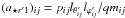
In Paper II the total acceleration a′ of a surface element, measured in
the non-inertial frame, is shown to be ![Mathematical equation: \begin{eqnarray} {\bf a}'& =& {\bf a}_{\star}- \frac{Gm_1 {\bf r}'}{|{\bf r}'|^3}-Gm_2 \left [ \frac{{\bf r}'- {\bf r}_{21}} {|{\bf r}'- {\bf r}_{21}|^3}+ \frac{{\bf r}_{21}} {|{\bf r}_{21}|^3} \right ] \nonumber \\ \label{ecmov} && - {\bf {\Omega}} \times \left ( {\bf \Omega} \times {\bf r}' \right ) -2 {\bf {\Omega}} \times \vec{v}'- \frac{{\rm d} {\bf {\Omega}}}{{\rm d}t} \times {\bf r}', \end{eqnarray}](/articles/aa/full_html/2011/04/aa15874-10/aa15874-10-eq27.png) (1)with
a⋆ the acceleration of a surface element
produced by gas pressure and viscous forces exerted by the stellar material surrounding the
element, and r′, v′ the position and velocity
of the element in the non-inertial frame. A nearly spherical shape is assumed for
m1 throughout its motion.
(1)with
a⋆ the acceleration of a surface element
produced by gas pressure and viscous forces exerted by the stellar material surrounding the
element, and r′, v′ the position and velocity
of the element in the non-inertial frame. A nearly spherical shape is assumed for
m1 throughout its motion.
The computation starts at time t = 0 with no relative motion between the
surface elements, so that at this initial time the acceleration
a⋆, with value
a⋆0, has only the contribution of gas
pressure. To compute this acceleration we consider a second, double-primed, non-inertial
reference frame, whose origin is also at the center of m1, and
has axes rotating with the assumed constant angular velocity
ω⋆ of the inner rigid region of star 1.
This angular velocity is written as
ω ⋆ = β0Ω0,
that is, equal to a certain fraction β0 of the initial orbital
angular velocity3.
The condition for initial equilibrium  on the
surface of m1 is (with
r′′ = r′)
on the
surface of m1 is (with
r′′ = r′) ![Mathematical equation: \begin{eqnarray} {\bf a}_{{\star}o}& =& \left \{ \frac{Gm_1 {\bf r}'}{|{\bf r}'|^3}+Gm_2 \left [ \frac{{\bf r}'- {\bf r}_{21}}{|{\bf r}'- {\bf r}_{21}|^3}+ \frac{{\bf r}_{21}}{|{\bf r}_{21}|^3} \right ] \right \}_{t=0} \nonumber\\ \label{aeso} && +\,\beta^2_0 {\bf {\Omega}}_0 \times \left ( {\bf {\Omega}}_0 \times {\bf r}'_0 \right ). \end{eqnarray}](/articles/aa/full_html/2011/04/aa15874-10/aa15874-10-eq39.png) (2)The
initial position r
(2)The
initial position r of a
surface element is obtained with an initial spherical shape of star 1, and its initial
velocity is,
of a
surface element is obtained with an initial spherical shape of star 1, and its initial
velocity is,  ×
r.
×
r.
The contribution of the m2- term in Eq. (2) makes a⋆0 in a given parallel have a non-constant azimuthal component. Thus the assumed initial spherical shape would not be the proper shape consistent with this azimuthal behavior. In our computations, at t = 0 we impose only the radial equilibrium resulting from Eq. (2), and allow unbalanced forces in the azimuthal direction. We found that with appropriate parameters (e.g. viscosity) this non-equilibrium initial condition will be followed by a transient phase and a steady state (dependent on the orbital phase) at later times.
At t > 0 the acceleration produced by gas pressure is conveniently
written in terms of the radial component of
a⋆0. Thus the radial component in Eq. (2), which is used in the following section, is
![Mathematical equation: \begin{eqnarray} a_{{\star}0r'} &= &\frac{Gm_1}{{r'_0}^2}+ Gm_2 \left [ \frac{r'_0-{r_{21}}_0\sin{\theta}'\cos{\varphi}'_0} {\left ({r'_0}^2+{r^2_{21}}_0-2r'_0{r_{21}}_0\sin{\theta}' \cos{\varphi}'_0 \right )^{3/2}}\right] \nonumber\\ \label{aesor} &&+ \,Gm_2 \left [\frac{\sin{\theta}'\cos{\varphi}'_0}{{r^2_{21}}_0}\right ]- {\beta}_0^2{\Omega}_0^2r'_0\sin^2{\theta}', \end{eqnarray}](/articles/aa/full_html/2011/04/aa15874-10/aa15874-10-eq44.png) (3)with
θ′ the polar angle of the given parallel and
(3)with
θ′ the polar angle of the given parallel and
 the initial
azimuthal angle of the element.
the initial
azimuthal angle of the element.
2.1. The acceleration a⋆
An element on the stellar surface of m1 has lateral surfaces
facing in the three directions of spherical coordinates, r′,
ϕ′, θ′ in the primed non-inertial frame. The
x′-axis points to m2 and
ϕ′ = 0 on the positive side of this axis; the polar axis is
z′, which is also the stellar rotation axis. We will denote with
i the parallel’s number and with j the number of the
element. The lengths of an element in the three directions are
 ,
,
 , and
, and
 , with
initial values
, with
initial values  ,
,
 ,
,
 . The
length is
assumed constant in time for all elements in a given parallel. In our scheme, for a given
element at any time is the
mean of its azimuthal distances to the centers of mass of the two adjacent elements in
this azimuthal direction, and is
twice the distance between the center of mass of the element and the boundary of the inner
stellar region. At t = 0 all the elements in a given parallel have the
same lengths.
. The
length is
assumed constant in time for all elements in a given parallel. In our scheme, for a given
element at any time is the
mean of its azimuthal distances to the centers of mass of the two adjacent elements in
this azimuthal direction, and is
twice the distance between the center of mass of the element and the boundary of the inner
stellar region. At t = 0 all the elements in a given parallel have the
same lengths.
The acceleration a⋆ has contributions from gas pressure and viscous shear. Below we describe the components of these contributions in spherical coordinates.
2.1.1. Gas pressure
The gas pressure inside a surface element is
pij, and we assume a polytropic state
equation
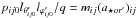
pij = pij0(ρij/ρij0)γ′,
with γ′ = 1 + 1/n; n is the
polytropic index and ρ the mass density. The pressure on the element
exerted by the neighboring stellar inner region is taken as
pint = pij/q,
0 < q < 1. We consider in particular the half value
q = 0.5. Thus the initial radial equilibrium is
 , with
mij the constant mass of the element. At
t > 0 the radial pressure acceleration is
, with
mij the constant mass of the element. At
t > 0 the radial pressure acceleration is
 . This
relation combined with the polytropic equation, the initial radial equilibrium, and with
the constant value of ,
gives
. This
relation combined with the polytropic equation, the initial radial equilibrium, and with
the constant value of ,
gives  (4)The azimuthal gas
pressure acceleration on a given element,
(a ⋆ ϕ′1)ij,
is computed with the difference of the gas pressure forces exerted by the two adjacent
elements in this azimuthal direction. Then
(4)The azimuthal gas
pressure acceleration on a given element,
(a ⋆ ϕ′1)ij,
is computed with the difference of the gas pressure forces exerted by the two adjacent
elements in this azimuthal direction. Then  . With the
polytropic form for each pressure, the corresponding initial radial equilibrium
conditions on the adjacent elements, and the same initial mass density for each surface
element (thus the same mass of elements in the given parallel, because their initial
lenghts are the same), this expression is
. With the
polytropic form for each pressure, the corresponding initial radial equilibrium
conditions on the adjacent elements, and the same initial mass density for each surface
element (thus the same mass of elements in the given parallel, because their initial
lenghts are the same), this expression is ![Mathematical equation: \begin{eqnarray} (a_{{\star}{\varphi}'1})_{ij}& =& q \frac{l_{r'_{ij}}}{l_{{\varphi}'_{ij0}}} \left [ l_{r'_{ij0}}l_{{\varphi}'_{ij0}} \right ]^{{\gamma}'} \nonumber \\ \label{aesfi1} &&\hspace{-11mm}\times \,\left \{(a_{{\star}0r'})_{i,j-1}\left [ l_{r'_{i,j-1}}l_{{\varphi}'_{i,j-1}} \right ]^{-{\gamma}'} \!\! -\! (a_{{\star}0r'})_{i,j+1}\left [ l_{r'_{i,j+1}}l_{{\varphi}'_{i,j+1}} \right ]^{-{\gamma}'} \right \}. \end{eqnarray}](/articles/aa/full_html/2011/04/aa15874-10/aa15874-10-eq73.png) (5)
(5)
2.1.2. Viscous force
The shear part of the kinematic stress tensor is given by (e.g., Symon 1971) ![Mathematical equation: \begin{equation} \vec{P}_{\eta} = -{\eta} \left [ {\nabla}' \vec{v}' + \left ( {\nabla}' \vec{v}' \right )^{\rm trp} - \frac{2}{3} {\bf 1} \left ({\nabla}' \cdot \vec{v}' \right ) \right ], \label{tensor} \end{equation}](/articles/aa/full_html/2011/04/aa15874-10/aa15874-10-eq74.png) (6)where
1 is the unit matrix, trp indicates the transposed, and
η is the coefficient of dynamic viscosity, related with the
coefficient of kinematic viscosity, ν, by
η = νρ, with ρ the mass density.
The total force on a given surface element from shear stresses is
(6)where
1 is the unit matrix, trp indicates the transposed, and
η is the coefficient of dynamic viscosity, related with the
coefficient of kinematic viscosity, ν, by
η = νρ, with ρ the mass density.
The total force on a given surface element from shear stresses is
 ,
with the integration over its surface. We picture each element with lateral faces in the
three directions of spherical coordinates, and corresponding lateral areas
Ar′,
Aϕ′,
Aθ′. Because we do not compute the
motion in the polar direction, with
,
with the integration over its surface. We picture each element with lateral faces in the
three directions of spherical coordinates, and corresponding lateral areas
Ar′,
Aϕ′,
Aθ′. Because we do not compute the
motion in the polar direction, with  , the relevant radial
and azimuthal components of the viscous force are
, the relevant radial
and azimuthal components of the viscous force are ![Mathematical equation: \begin{eqnarray} (F_{\eta})_{r'} &=& A_{r'}{\Delta}\left [\eta \left ( \frac{4}{3}r'\frac{\partial}{\partial r'}\left ( \frac{v'_{r'}}{r'} \right )-\frac{2}{3}\frac{\partial {\omega}'}{\partial {\varphi}'} \right ) \right ]\nonumber \\ &&+ A_{{\varphi}'}{\Delta} \left [\eta \left ( r' \frac{\partial {\omega}'}{\partial r'}\sin{\theta}'+ \frac{1}{r'\sin{\theta}'}\frac {\partial v'_{r'}}{\partial {\varphi}'} \right ) \right ] \nonumber\\ \label{frvis} && + A_{{\theta}'}{\Delta} \left [ \frac{\eta}{r'} \frac{\partial v'_{r'}}{\partial {\theta}'} \right ], \\ (F_{\eta})_{{\varphi}'} &=& A_{r'}{\Delta}\left [\eta \left ( r'\frac{\partial {\omega}'}{\partial r'}\sin{\theta}'+ \frac{1}{r'\sin{\theta}'}\frac {\partial v'_{r'}}{\partial {\varphi}'} \right ) \right ]\nonumber \\ &&+ A_{{\varphi}'}{\Delta} \left [\eta \left ( -\frac{2}{3}r' \frac {\partial}{\partial r'}\left ( \frac{v'_{r'}} {r'} \right ) + \frac{4}{3}\frac{\partial {\omega}'}{\partial {\varphi}'} \right ) \right ]\nonumber \\ \label{ffivis} && + A_{{\theta}'}{\Delta} \left [\eta \frac{\partial {\omega}'}{\partial {\theta}'}\sin{\theta}' \right ], \end{eqnarray}](/articles/aa/full_html/2011/04/aa15874-10/aa15874-10-eq85.png) with
Δ meaning the difference of values of the function inside a square parenthesis computed
at the corresponding lateral faces in the direction given by the lateral area factor.
with
Δ meaning the difference of values of the function inside a square parenthesis computed
at the corresponding lateral faces in the direction given by the lateral area factor.
In our macroscopic element description, for the evaluation of the several terms in this
surface integration we consider as important the gradients across the
lateral faces of an element and ignore local gradients along these
faces. Thus, given that the density drops to zero at the outer face and the radial
velocity is also zero at the inner rigid region, we approximate the radial and azimuthal
components of the viscous force as ![Mathematical equation: \begin{eqnarray} \label{apfrvis} (F_{\eta})_{r'} &\simeq & A_{{\varphi}'}{\Delta} \left [ \frac{\eta}{r'\sin{\theta}'}\frac {\partial v'_{r'}}{\partial {\varphi}'} \right ] + A_{{\theta}'}{\Delta} \left [\frac{\eta}{r'} \frac{\partial v'_{r'}}{\partial {\theta}'} \right ], \\ (F_{\eta})_{{\varphi}'} &\simeq & -A_{r'}\left [\eta r'\frac{\partial {\omega}'}{\partial r'}\sin{\theta}' \right ] + \frac{4}{3}A_{{\varphi}'}{\Delta} \left [\eta \frac{\partial {\omega}'}{\partial {\varphi}'} \right ] \nonumber\\ \label{apffivis} && +A_{{\theta}'}{\Delta} \left [\eta \frac{\partial {\omega}'}{\partial {\theta}'}\sin{\theta}' \right ], \end{eqnarray}](/articles/aa/full_html/2011/04/aa15874-10/aa15874-10-eq89.png) with
the first term in Eq. (10) computed at
the boundary with the inner rigid region.
with
the first term in Eq. (10) computed at
the boundary with the inner rigid region.
The terms in Eq. (9) give second and
third contributions to the radial acceleration, besides that in Eq. (4). Taking the coefficient of kinematic
viscosity, ν, to be the same in all the elements, the acceleration
corresponding to the first term is approximated as in Eq. (11) of Paper II ![Mathematical equation: \begin{equation} (a_{{\star}r'2})_{ij} \simeq \frac{\nu} {l^2_{{\varphi}'_{ij}}} \left [ v'_{{r'}_{i,j+1}} + v'_{{r'}_{i,j-1}} -2 v'_{{r'}_{ij}} \right ], \label{aesr2} \end{equation}](/articles/aa/full_html/2011/04/aa15874-10/aa15874-10-eq90.png) (11)likewise, the second
term in Eq. (9) gives the acceleration
(11)likewise, the second
term in Eq. (9) gives the acceleration
![Mathematical equation: \begin{equation} (a_{{\star}r'3})_{ij} \simeq \frac{\nu} {l^2_{{\theta}'_{ij}}} \left [ v'^{\ast}_{{r'}_{i+1,j}} + v'^{\ast}_{{r'}_{i-1,j}} -2 v'_{{r'}_{ij}} \right ], \label{aesr3} \end{equation}](/articles/aa/full_html/2011/04/aa15874-10/aa15874-10-eq91.png) (12)with
(12)with
 ,
,
 the mean radial velocities of the elements in the polar direction adjacent to the
element ij.
the mean radial velocities of the elements in the polar direction adjacent to the
element ij.
In the first term of Eq. (10) we
approximate 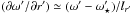 , with
 the
angular velocity of the inner stellar region as measured in the primed non-inertial
frame. In the second term we make a similar approximation as that used to obtain
Eq. (11) and ignore the factor 4/3.
Thus, the corresponding accelerations are
the
angular velocity of the inner stellar region as measured in the primed non-inertial
frame. In the second term we make a similar approximation as that used to obtain
Eq. (11) and ignore the factor 4/3.
Thus, the corresponding accelerations are ![Mathematical equation: \begin{eqnarray} \label{aesfi2} (a_{{\star}{\varphi}'2})_{ij} &\simeq& - \frac{\nu} {l^2_{r'_{ij}}} \left( r'_{ij}- \frac{1}{2}l_{r'_{ij}}\right) \left [ \frac {v'_{{\varphi}'_{ij}}}{r'_{ij}} - \left ( {\beta}_0{\Omega}_0 - \Omega \right )\sin{\theta}'_i \right ], \\ \label{aesfi3} (a_{{\star}{\varphi}'3})_{ij} &\simeq& \frac{\nu} {l^2_{{\varphi}'_{ij}}} \left [ v'_{{\varphi}'_{i,j+1}} + v'_{{\varphi}'_{i,j-1}} - 2 v'_{{\varphi}'_{ij}} \right ], \end{eqnarray}](/articles/aa/full_html/2011/04/aa15874-10/aa15874-10-eq97.png) and
finally, the last term in Eq. (10) gives
the azimuthal acceleration
and
finally, the last term in Eq. (10) gives
the azimuthal acceleration ![Mathematical equation: \begin{equation} (a_{{\star}{\varphi}'4})_{ij}\! \simeq\! \frac {{\nu}r'_{ij}}{l^2_{{\theta}'_{ij}}}\! \left [ ({\omega}'^{\ast}_{i+1,j}\!-\!{\omega}'_{ij})\sin{\theta}'_{i,i+1}\!-\! ({\omega}'_{ij}\!-\!{\omega}'^{\ast}_{i-1,j})\sin{\theta}'_{i-1,i} \right ], \label{aesfi4} \end{equation}](/articles/aa/full_html/2011/04/aa15874-10/aa15874-10-eq98.png) (15)with
(15)with
 ,
,
 the mean angular velocities of the elements in the polar direction adjacent to the
element ij, and
the mean angular velocities of the elements in the polar direction adjacent to the
element ij, and  ,
,
 the polar
angles of the boundaries of the adjacent parallels.
the polar
angles of the boundaries of the adjacent parallels.
2.2. Equations of motion
The acceleration a⋆ of a surface element
produced by gas pressure and viscous forces has a radial component
a⋆r′ given by the sum of Eqs. (4), (11), and (12), and the
corresponding azimuthal component a⋆ϕ′ is the sum of
Eqs. (5), (13), (14), and (15). In the primed non-inertial reference
frame, the pair of radial and azimuthal equations of motion of a surface element are
![Mathematical equation: \begin{eqnarray} \ddot{r}' & = & -\, \frac{Gm_1}{{r'}^2}- Gm_2 \Bigg [ \frac{r'-r_{21}\sin{\theta}'\cos{\varphi}'} {\left ({r'}^2+r^2_{21}-2r'r_{21}\sin{\theta}'\cos{\varphi}' \right )^{3/2}} \nonumber \\ &&+\,\frac{\sin{\theta}'\cos{\varphi}'}{r^2_{21}} \Bigg ] + a_{{\star}r'}+(\Omega + \dot{\varphi}')^2r'\sin^2{\theta}', \label{emr} \\ \ddot{\varphi}' & = & \frac{1}{r'\sin{\theta}'} \left \{ a_{{\star}{\varphi}'}- Gm_2 \left [ \frac{r_{21}} {\left ({r'}^2+r^2_{21}-2r'r_{21}\sin{\theta}'\cos{\varphi}' \right )^{3/2}}\right.\right. \nonumber \\&&\left.\left.\phantom{\frac{r_{21}} {\left ({r'}^2+r^2_{21}-2r'r_{21}\sin{\theta}'\cos{\varphi}' \right )^{3/2}}}\hspace{-4.9cm}-\, \frac{1}{r^2_{21}} \right ]\sin{\varphi}' \right \} -\dot{\Omega} - \frac{2}{r'}(\Omega + \dot{\varphi}')\dot{r}'. \label{emfi} \end{eqnarray}](/articles/aa/full_html/2011/04/aa15874-10/aa15874-10-eq105.png) All
pairs of equations in all surface elements are solved simultaneously, along with the
orbital motion of m2 around m1.
The values of r21, Ω,
All
pairs of equations in all surface elements are solved simultaneously, along with the
orbital motion of m2 around m1.
The values of r21, Ω,  are obtained from this orbital motion. We used a seventh-order Runge-Kutta algorithm
(Fehlberg 1968) to solve the equations. With some
forty parallels covering the stellar surface, more than 104 elements are
employed.
are obtained from this orbital motion. We used a seventh-order Runge-Kutta algorithm
(Fehlberg 1968) to solve the equations. With some
forty parallels covering the stellar surface, more than 104 elements are
employed.
2.3. Method for Ė calculation
The rate of energy dissipation per unit volume can be expressed in terms of the tensor in
Eq. (6), and is given by the matrix product
(e.g., McQuarrie 1976) 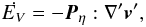 (18)which can be written as
![Mathematical equation: \begin{equation} \dot{E_V} = -2\eta \left [\frac{1}{3} \left ({\nabla}' \cdot \vec{v}' \right )^2 - \left ( {\nabla}' \vec{v}' \right )_s : \left ( {\nabla}' \vec{v}' \right )_s \right ], \label{dis2} \end{equation}](/articles/aa/full_html/2011/04/aa15874-10/aa15874-10-eq110.png) (19)where
(19)where
 is
the symmetric tensor
is
the symmetric tensor ![Mathematical equation: \hbox{$({\nabla}'\vec{v}')_{\rm s} = \frac{1}{2} [{\nabla}'\vec{v}'+ ({\nabla}'\vec{v}')^{\rm trp}]$}](/articles/aa/full_html/2011/04/aa15874-10/aa15874-10-eq112.png) .
.
The computations in our model show that the gradient in azimuthal velocity dominates that
in radial velocity. Thus, Eq. (19) can be
approximated as 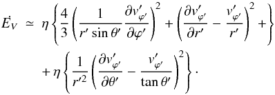 (20)Now
with , it follows that
(20)Now
with , it follows that
 (21)
(21) (22)
(22) (23)and Eq. (20) reduces to
 ![Mathematical equation: \begin{equation} \dot{E_V} \simeq {\eta} \left \{ \frac{4}{3} \left ( \frac{\partial {\omega}'}{\partial {\varphi}'} \right )^2 + \left [ r'^2 \left ( \frac{\partial {\omega}'}{\partial r'} \right )^2 + \left ( \frac{\partial {\omega}'}{\partial {\theta}'} \right )^2 \right ]{\sin}^2{\theta}' \right \}. \label{dis4} \end{equation}](/articles/aa/full_html/2011/04/aa15874-10/aa15874-10-eq117.png) (24)For an accretion disk
(θ′ = π/2, and the primed reference frame is taken
as inertial in this case) with ω′ a function only of the radial distance
r′, and
(24)For an accretion disk
(θ′ = π/2, and the primed reference frame is taken
as inertial in this case) with ω′ a function only of the radial distance
r′, and  small compared
with
small compared
with  , Eq. (24) gives
 (Lynden-Bell
& Pringle 1974); this result was used in
Eq. (14) of Toledano et al. (2007), multiplied by
the volume of an element.
(Lynden-Bell
& Pringle 1974); this result was used in
Eq. (14) of Toledano et al. (2007), multiplied by
the volume of an element.
The j-surface element on the parallel with polar angle
 has a volume

 , with
 and
and
 . The rate of
energy dissipation in the element is
Ėij = ĖVijΔVij,
with ĖVij the evaluation of Eq. (24) at the position of the element.
. The rate of
energy dissipation in the element is
Ėij = ĖVijΔVij,
with ĖVij the evaluation of Eq. (24) at the position of the element.
As already done to approximate Eq. (10),
we take 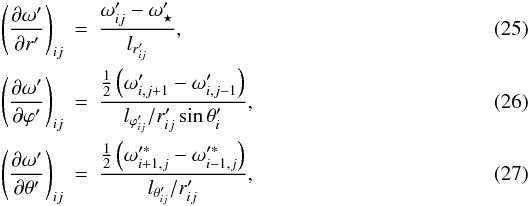 Eqs.
(25)–(27) are inserted in Eq. (24), giving ĖVij which has three
contributions
(ĖVij)r′,
(ĖVij)ϕ′, and
(ĖVij)θ′,
corresponding to the three gradients of angular velocity in spherical coordinates. The
total rate of energy dissipation in the surface layer is
Eqs.
(25)–(27) are inserted in Eq. (24), giving ĖVij which has three
contributions
(ĖVij)r′,
(ĖVij)ϕ′, and
(ĖVij)θ′,
corresponding to the three gradients of angular velocity in spherical coordinates. The
total rate of energy dissipation in the surface layer is ![Mathematical equation: \begin{equation} {\dot{E}} = \sum_{i,j}^{} \left [\left ({\dot{E}}_{Vij} \right )_{r'} + \left ({\dot{E}}_{Vij} \right )_{{\varphi}'} + \left ({\dot{E}}_{Vij} \right )_{{\theta}'} \right ]{\Delta}V_{ij}. \label{etot} \end{equation}](/articles/aa/full_html/2011/04/aa15874-10/aa15874-10-eq134.png) (28)In our computations the
major contribution to Ė comes from
(ĖVij)r′.
(28)In our computations the
major contribution to Ė comes from
(ĖVij)r′.
3. Energy dissipation rates
3.1. Sample Ė(ϕ′,θ′) calculation
We can compute Ėij, the rate of energy
dissipation in the element j in a given parallel i, as a
function of the azimuthal angle ϕ′ of the element. Also, it is of
interest to compute Ėi, the total rate of
energy dissipation in the parallel i, as a function of the corresponding
polar angle θ′. As an example, in this section we show results from our
model in the particular polytropic case with n = 1.5 and using a surface
layer depth ΔR1/R1 = 0.03, with
corresponding average mass density
ρ = 8.66 × 10⁻⁷ gr cm-3. The other input
parameters are M1 = 5 M⊙,
M2 = 4 M⊙,
R1 = 3.2 R⊙,
 day-1,
an orbital period P = 10 days
(a = 40.62 R⊙), and with two different
values β0 = 1.2 and 2.
day-1,
an orbital period P = 10 days
(a = 40.62 R⊙), and with two different
values β0 = 1.2 and 2.
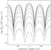 |
Fig. 1 Rate of energy dissipation Ėij as a
function of ϕ′ in a few selected parallels, for the
n = 1.5 polytropic case
ΔR1/R1 = 0.03,
ν = 0.003 |
Figure 1 shows the run of Ėij as a function of ϕ′ in some selected parallels for β0 = 1.2. The upper curve corresponds to the stellar equator, θ′ = 90°, and following curves from top to bottom give results for the parallels with θ′ ≈ 81°, 73°, 64°, 55°, 46°, 38°, 29° and 20°. A very similar results is obtained for the β0 = 2 calculation, although the energy dissipation rates are significantly larger.
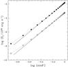 |
Fig. 2 Rate of energy dissipation in the parallel i as a function of its polar angle, corresponding to the computations in Fig. 1. Results with β0 = 1.2 and 2 are shown with empty and filled squares, respectively. The continuous lines show functions with a sin7θ′ dependence. |
Figure 2 shows the total rate of energy dissipation
in the parallel i, Ėi, as a
function of its polar angle. Both cases β0 = 1.2 and 2 are
shown in this figure, with empty and filled squares, respectively. The continuous lines
show functions with a sin7θ′ dependence. Thus, our
computations give the approximate dependence  , excluding polar
angles in a region of approximately 10° around the poles. This implies that in our model
, excluding polar
angles in a region of approximately 10° around the poles. This implies that in our model
 has a
has a
 dependence, thus
the dominant radial gradient in Eq. (24)
integrated in the volume of the parallel, which has a
dependence, thus
the dominant radial gradient in Eq. (24)
integrated in the volume of the parallel, which has a
 dependence, gives
. Concerning this
result, there is a theoretical study by Scharlemann (1981), which gives the tidal velocity field in a differentially rotating
convective envelope of a component in a binary system in circular relative orbit, in the
limit β0 → 1. For the case in which the star rotates
uniformly, Eq. (40c) of Scharlemann (1981) gives
the azimuthal component of the tidal velocity field. This equation implies, in our
notation,
dependence, gives
. Concerning this
result, there is a theoretical study by Scharlemann (1981), which gives the tidal velocity field in a differentially rotating
convective envelope of a component in a binary system in circular relative orbit, in the
limit β0 → 1. For the case in which the star rotates
uniformly, Eq. (40c) of Scharlemann (1981) gives
the azimuthal component of the tidal velocity field. This equation implies, in our
notation,  , which differs from
our result. Yet we find in our computations with β0 = 1.2, 2.0
that the surface layer does not rotate uniformly, contrary to the assumption in
Scharlemann’s equation. Thus, the difference between the two results most likely stems
from Scharlemann’s assumption of uniform rotation over the stellar surface which, for
β ≠ 1, is incorrect.
, which differs from
our result. Yet we find in our computations with β0 = 1.2, 2.0
that the surface layer does not rotate uniformly, contrary to the assumption in
Scharlemann’s equation. Thus, the difference between the two results most likely stems
from Scharlemann’s assumption of uniform rotation over the stellar surface which, for
β ≠ 1, is incorrect.
3.2. Dependence of Ė on orbital separation
In this section, we analyze the behavior of the total rate of energy dissipation, Ė for binary system models with different orbital separations and a variety of orbital eccentricities.
3.2.1. Circular orbits
As in Toledano et al. (2007), we adopt as the
test binary system one with masses
m1 = 5 M⊙ and
m2 = 4 M⊙;
m1 with a radius
R1 = 3.2 R⊙. The analysis
was made for circular relative orbits with several different values of orbital
separation a. The energy dissipation rate given by Eq. (28) was computed in
m1; we used 20 parallels distributed between the equator
and polar angle 85°, with more than 104 surface elements, and a polytropic
index n = 1.5. In the coefficient of dynamic viscosity
η = νρ the same approach as that of Toledano et al.
(2007) was adopted. That is, the average mass
density for the surface layer,
ΔR1/R1, is taken from a BEC
stellar structure model computation4. For this
paper we used a model5 kindly provided by Brott
(2010, priv. comm.). The value of the kinematic viscosity ν was taken
as the lowest value allowed by the code (see discussion in Harrington et al. 2009, regarding this parameter). For the shortest
period binary models with circular orbits, this value is
ν = 0.003  day-1, which we adopted for the whole set of circular orbit models
discussed in this section. Three different values of the thickness of the surface layer
in m1 were considered,
ΔR1/R1 = 0.01, 0.03,
0.066. The corresponding average mass densities
are, 1.19 × 10⁻⁸, 1.68 × 10⁻⁷ and
8.66 × 10⁻⁷ g cm-3, respectively. The computations were made for
two values β0 = 1.2, 2.0 of the synchronicity parameter.
day-1, which we adopted for the whole set of circular orbit models
discussed in this section. Three different values of the thickness of the surface layer
in m1 were considered,
ΔR1/R1 = 0.01, 0.03,
0.066. The corresponding average mass densities
are, 1.19 × 10⁻⁸, 1.68 × 10⁻⁷ and
8.66 × 10⁻⁷ g cm-3, respectively. The computations were made for
two values β0 = 1.2, 2.0 of the synchronicity parameter.
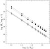 |
Fig. 3 Energy dissipation in m1 as a function of the separation a of the circular orbit. A polytropic index n = 1.5 is used. Empty symbols correspond to β0 = 1.2 and filled symbols to β0 = 2.0. The correspondence with the layer thickness ΔR1/R1 is, in triangles: ΔR1/R1 = 0.01, in squares: ΔR1/R1 = 0.03, in pentagons: ΔR1/R1 = 0.06. The continuous line is a function with an a-9 dependence on a. |
Figure 3 shows the energy dissipation Ė in m1 as a function of the radius of the circular orbit. Empty symbols correspond to β0 = 1.2 and filled symbols to β0 = 2.0. Triangles, squares, and pentagons show results for ΔR1/R1 = 0.01, 0.03, and 0.06, respectively. A clear linear behavior is obtained on this log-log plot. For comparison, the continuous line in this figure shows a function with an a-9 dependence on the orbital radius a. The data in the three cases ΔR1/R1 would shift vertically for different values of the mass density and viscosity, but the functional dependence on orbital separation remains the same.
3.2.2. Elliptic orbits
Elliptical orbit binary systems differ from those in circular orbits in that the synchronicity parameter, β, does not remain constant over the orbital cycle. This is because of the variation of the orbital angular velocity, Ω. The computation takes into account the changing value of β, but we characterize each model by its synchronicity parameter at periastron, β0.
The energy dissipation rates for a grid of elliptical orbit binary systems were
computed following a similar procedure as in Sect. 3.2.1 for the
m1 + m2 = 5 + 4 M⊙
binary system, but in this case eccentricities e = 0.1, 0.3, 0.5 0.7
and 0.8 were assigned, and 20 latitude grid points were used in each hemisphere of
m1. The remaining parameters were held constant:
R1 = 3.2, β0 = 1.2,
ΔR1/R1 = 0.06,
n = 1.5,  day-1.
The changing separation of the two stars over the orbital cycle leads to a strong
dependence of the energy dissipation rate on the orbital phase. Thus, in order to assign
a value of Ė to each model calculation, an average value of the energy
dissipation rate over orbital cycle, Ėave, was computed by
numerically integrating Ė obtained at many phases distributed over the
orbital cycle, and then dividing by the corresponding orbital period. The values of
Ėave are plotted in Fig. 4 as a function of the major semi-axis of the orbit.
day-1.
The changing separation of the two stars over the orbital cycle leads to a strong
dependence of the energy dissipation rate on the orbital phase. Thus, in order to assign
a value of Ė to each model calculation, an average value of the energy
dissipation rate over orbital cycle, Ėave, was computed by
numerically integrating Ė obtained at many phases distributed over the
orbital cycle, and then dividing by the corresponding orbital period. The values of
Ėave are plotted in Fig. 4 as a function of the major semi-axis of the orbit.
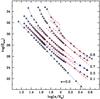 |
Fig. 4 Energy dissipation rates (in erg s-1) from our model calculations for β0 = 1.2 and different eccentricities as indicated. The dashed lines show the absolute value of Ėorb given by Eq. (A31) of Hut (1981), as written in our Eq. (30). The dotted lines connect the points corresponding to each eccentricity. The short dot-dashed lines show the values of ĖHut for e = 0.8 and lag angles α = 10° and 50°. |
Two aspects of this figure stand out: 1) there is a “family” of curves, one for each value of the eccentricity; 2) in each case, the scaling of Ėave with a does not follow a unique linear (in the log-log plane) plot, as in the circular orbit case. Instead, for very short orbital periods, the slope is steeper and for very long periods, the slope is flatter than the Ėave ~ a-9 relation for circular orbits. It is also interesting to note that the departure from this relation grows with increasing orbital eccentricity.
3.3. Comparison with the “weak friction” model
Hut (1981) provided a derivation of the differential equations for the tidal evolution under the “weak friction, equilibrium tide” model representation for the tidal interaction (Darwin 1880; Alexander 1973). The fundamental assumption of this model is that the tidal bulges that are raised by the external perturbing potential are only slightly misaligned with respect to the axis that connects the two stars. The system is then driven toward an equilibrium configuration through the action of the torques acting on the “retarded body”. The misalignment of the bulges is caused by dissipation (i.e., friction) in the perturbed star. Hut’s formalism includes high order terms in the orbital eccentricity, as required to properly assess the energy dissipation rates in very eccentric systems7. In this section we test our model by computing the energy dissipation rates for a 5 + 4 M⊙ polytropic (n = 1.5) binary system with a primary star’s radius R1 = 3.2 R⊙ for a range in orbital separations and eccentricities. Each binary system of the grid is characterized by the energy dissipation rates averaged over the orbital cycle, Ėave. We show that for a variety of orbital eccentricities, the behavior of Ėave is consistent with the predicted energy dissipation rates in the “weak friction” approximation given by Hut (1981) within the domain of applicability of this approximation. Our model also adequately predicts the pseudo-synchronization angular velocity obtained by Hut (1981) for moderate eccentricities (e ≤ 0.3).
3.3.1. Energy dissipation rates
The rate of energy dissipation within the primary star associated with the decrease in
the orbital and rotation energy in the system is given by Hut (1981) in his Eq. (A31)
![Mathematical equation: \begin{eqnarray} \dot{E}_{\rm Hut} = -3 \frac{k}{T} G(m_1\!+\!m_2)\left ( \frac{m_2^2}{m_1} \right ) \left(\frac{R_1^8}{a^9}\right ) (1\!-\!e^2 )^{-15/2} \left [A\!-\!2Bx\!+\!Cx^2 \right ] \nonumber \end{eqnarray}](/articles/aa/full_html/2011/04/aa15874-10/aa15874-10-eq195.png) (28)where
k is a constant that depends on the stellar structure, and
x = ω/n, with ω
the angular rotation velocity of m1 and
n = np(1 − e2)3/2/(1 + e)2
the mean orbital angular velocity, with np the orbital
angular velocity at periastron.
(28)where
k is a constant that depends on the stellar structure, and
x = ω/n, with ω
the angular rotation velocity of m1 and
n = np(1 − e2)3/2/(1 + e)2
the mean orbital angular velocity, with np the orbital
angular velocity at periastron.  ,
where τ is the lag time, and
,
where τ is the lag time, and
 (29)After
converting masses and distances to solar units, and writing
ω/n in terms of
np, and recalling that
ω/np = β0,
the above equation can be rewritten as
(29)After
converting masses and distances to solar units, and writing
ω/n in terms of
np, and recalling that
ω/np = β0,
the above equation can be rewritten as ![Mathematical equation: \begin{eqnarray} \dot{E}_{\rm Hut}& =& -4.4\times10^{42} k \tau \left ( \frac{m_1+m_2}{M_\odot} \right ) \left (\frac{m_2}{M_\odot} \right)^2 \left (\frac{R_1}{R_\odot} \right )^5 \left(\frac{a}{R_\odot} \right)^{-9} \nonumber \\ \label{eqhut2} &&\times (1-e^2)^{-15/2} \left [A - 2 Bx+Cx^2 \right ], \end{eqnarray}](/articles/aa/full_html/2011/04/aa15874-10/aa15874-10-eq206.png) (30)with
ĖHut given in erg s-1 and
x = β0(1 + e)2.
(30)with
ĖHut given in erg s-1 and
x = β0(1 + e)2.
For the lag time, Hut (1981, Eq. (4)) gives τ = α/(ω − Ω), where ω and Ω are the rotational and instantaneous orbital angular velocity, respectively. α is the lag angle, and is measured from the line that joins the centers of m1 and m2. This expression may be re-written in terms of the instantaneous synchronicity parameter, β, as τ = α/Ω(β − 1).
In eccentric binary systems, α is generally very small around
periastron, but it can be quite large at other orbital phases8. At the same time, the amplitude of the tidal bulges is largest
around periastron and, given that this is when m1 and
m2 have their closest approach, the tidal interaction
effects are strongest. Hence, for the purpose of these exploratory calculations, we now
make the following approximation: To compute the energy dissipation rates using
Eq. (30), we adopt
τ ~ αper/Ω0(β0 − 1),
where αper is the lag angle at periastron which we assume is
relatively small, and here tentatively adopt α = 1°. We thus also use
β = β0. Using Kepler’s relation
Ω0 = G1/2(m1 + m2)1/2a − 3/2(1 + e)2(1 − e2) − 3/2
and converting to solar units, 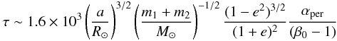 (31)with
αper given in radians and τ is in
seconds. Note that when Eq. (31) is
introduced into Eq. (30), the dependence
of ĖHut on orbital separation
~ a − 15/2, thus flattening the slope from the
a-9 relation that holds for a circular orbit.
(31)with
αper given in radians and τ is in
seconds. Note that when Eq. (31) is
introduced into Eq. (30), the dependence
of ĖHut on orbital separation
~ a − 15/2, thus flattening the slope from the
a-9 relation that holds for a circular orbit.
For the value of k, we use the expression given in Lecar et al. (1976,
their Eq. (2)) for the mass in the tidal bulge, Mt:
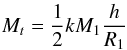 (32)where
h is the height of the tide. Consider, for example, the model binary
system with e = 0.8, P = 15 d, from the grid of models
discussed in the previous section. The height of the tide at periastron is
~ 0.03 R⊙ (see below). The mass in the bulge is
Mt = ftMlayer,
where ft is the fraction of the mass in the outer layer,
Mlayer, that goes into to the bulge. For the particular
case in question,
(32)where
h is the height of the tide. Consider, for example, the model binary
system with e = 0.8, P = 15 d, from the grid of models
discussed in the previous section. The height of the tide at periastron is
~ 0.03 R⊙ (see below). The mass in the bulge is
Mt = ftMlayer,
where ft is the fraction of the mass in the outer layer,
Mlayer, that goes into to the bulge. For the particular
case in question,  , where
ΔR1 = 0.06 R⊙ is the layer
thickness and ⟨ ρ ⟩ = 8.66 × 10⁻⁷ g cm-3, is
the average density of the layer. The maximum in the primary bulge approximately extends
over 20° in azimuth, so ft ~ 10-4.
Hence, this estimate yields k ~ 10-8.
, where
ΔR1 = 0.06 R⊙ is the layer
thickness and ⟨ ρ ⟩ = 8.66 × 10⁻⁷ g cm-3, is
the average density of the layer. The maximum in the primary bulge approximately extends
over 20° in azimuth, so ft ~ 10-4.
Hence, this estimate yields k ~ 10-8.
With these considerations, we use Eq. (30) to estimate the energy dissipation rates in the “weak friction” approximation, ĖHut, for the binary model parameters m1 = 5 M⊙, m2 = 4 M⊙, R1 = 3.2 R⊙, β0 = 1.2, and k = 5 × 10⁻⁸. The dashed lines in Fig. 4 correspond to the absolute values of ĖHut given by Eq. (30). The coincidence between the general behavior of these lines and that of the numerical computations is encouraging. Note that no relative shift or scaling is introduced, and yet the relative separation between the curves corresponding to the different eccentricities is reproduced by our models. In addition, our model reproduces the general trend in the slope of the Ėave vs. a relation, particularly for large orbital separations. Thus, we find that our numerical calculation captures to a large extent the general scaling in the energy dissipation rates predicted analytically within the “weak friction” tidal model.
However, although the scaling with e predicted by Eq. (30) is adequately captured by our model, the dependence on a − n, with n = const. is not satisfied. Specifically, there is a marked excess in Ėave for smaller orbital separations, with respect to ĖHut. Several factors may be responsible for this difference. First, the assumption of a constant lag angle, α, is quite inadequate. For example, assuming that for the e = 0.8 calculation α = 10° and 50°, instead of the 1° used to draw the dash lines, significantly higher ĖHut values are obtained9. This is illustrated by the short dashed lines in Fig. 4. Second, the applicability of the standard “equilibrium tide” model for high eccentricities is questionable (Efroimsky & Williams 2009). Finally, we note that our model assumes a spherical rigidly-rotating interior region, and that this approximation is less applicable for small orbital separations, where the deformation of the star is greater.
 |
Fig. 5 Energy dissipation rates of the previous figure but here plotted as a function of the periastron distance, rper. In this representation, the different curves for each eccentricity “collapse” onto a common region. The dashed lines show the absolute value of Ėorb given by Eq. (A31) of Hut (1981) for e = 0.1 and 0.8, also plotted as a function of rper. Symbols correspond to the different eccentricities: e = 0.00 (open triangles), 0.01 (filled triangles), 0.10 (small pentagons), 0.30 (large pentagons), 0.50 (crosses), 0.70 (stars) and 0.8 (filled pentagons). |
It is interesting to note that if Ė is plotted as a function of rper, the orbital separation at periastron, instead of the semi-major axis, the curves corresponding to the different eccentricities “collapse” toward a single curve. This is illustrated in Fig. 5. Thus, the periastron distance is a more convenient parameter for the purpose of analyzing the average energy dissipation rates than the semi-major axis.
3.3.2. Pseudo-synchronization angular velocity
Pseudo-synchronization in an eccentric binary is a term used to describe the state that is closest to an equilibrium configuration. Hut (1981) demonstrated that the rotational angular velocity for pseudo-synchronization, ωps < Ω0, where Ω0 is the orbital angular velocity at periastron. Specifically, 0.8 < ωps/Ω0 < 110.
We computed sets of models with e = 0.1, 0.3, 0.5 (P = 6 d) and 0.8 (P = 20 d) holding all other parameters fixed except for β0, which was varied from ~ 0.4 to the highest value admitted by the calculation.11 Figure 6 illustrates the dependence of Ėave on β0. In all cases, there is a minimum in Ėave at a particular value (or range of values) of β0. For e = 0.1 and 0.3, the minimum occurs around β0 ~ 0.8–0.9, consistent with the “weak friction” approximation. For e = 0.5 and 0.8, however, the minimum occurs for 1.0 < β0 < 1.4, a result that is likely related to the caveats already mentioned at the end of the previous section.
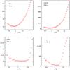 |
Fig. 6 Energy dissipation rates Ėave/1035 ⟨ ρ ⟩ as a function of β0 = ω/Ω0 for four different eccentricities, e = 0.1 (top left), 0.3 (top right), 0.5 (bottom left) and 0.8 (bottom right). The first three cases are for an orbital period P = 6 d and the last is for 20 d. The ordinate is in units of 1035 ⟨ ρ ⟩ erg s-1, where ⟨ ρ ⟩ is the average density. The dotted line indicates the level of minimum Ėave which, for e = 0.1 and 0.3 coincides with the analytical results of Hut (1981). |
4. Synchronization timescales
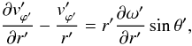
In this section we analyze the synchronization time scales, which will be defined below, using the model presented in Sect. 2, the procedure to compute the energy dissipation in Sect. 2.3, and the Ėave values described in the previous section. The results will be compared with the earlier results of Toledano et al. (2007) and with a theoretical result given by Zahn (1977, 2008).
4.1. Circular orbits
As in Toledano et al. (2007), we now procede to
estimate the synchronization time scale between the stellar rotation period and the
orbital period. The synchronization time scale is the time needed by the system to arrive
at a state in which both periods are equal, and this state is here assumed to be attained
as a consequence of the energy dissipation in the surface layer. In our computations, at
time t = 0 the whole star, including the surface layer, is rotating with
an angular velocity
ω ⋆ = β0Ω0,
with Ω0 the reference orbital angular velocity. For
circular orbits, Ω0 is directly the angular velocity
in the circular orbit while for e > 0 it is the angular velocity
at periastron. We adopt here as the condition for synchronicity12β0 = 1. Thus, with
β0 > 1 there is an initial excess of rotational
kinetic energy over that in the synchronized state. As a first approximation, ignoring the
orbital change suffered by the binary system to reach the
β0 = 1 state, the excess of rotational kinetic energy is
proportional to  , with the
proportionality constant being I/2, with I the moment
of inertia. Thus for star m1 the synchronization time is on
the order of
, with the
proportionality constant being I/2, with I the moment
of inertia. Thus for star m1 the synchronization time is on
the order of  (33)From Kepler’s
law,
(33)From Kepler’s
law,  has an
a-3 dependence on the major semi-axis a.
Thus, for a fixed value of β0 and with the approximate
a-9 dependence of Ė from Fig. 3, τsyn will have an
a6 dependence on a for circular orbits.
has an
a-3 dependence on the major semi-axis a.
Thus, for a fixed value of β0 and with the approximate
a-9 dependence of Ė from Fig. 3, τsyn will have an
a6 dependence on a for circular orbits.
On the other hand, Zahn (1977) has analyzed
theoretically the tidal friction in close binary stars, also arriving at an
a6 dependence for stars in which a turbulent viscosity may
be the main mechanism that produces the tidal friction. In a recent review of the topic
(Zahn 2008), this expression for circular orbits is
given as  (34)with
q = m2/m1,
I the moment of inertia of m1, Ω is the
orbital angular velocity which for circular orbits is constant.
(34)with
q = m2/m1,
I the moment of inertia of m1, Ω is the
orbital angular velocity which for circular orbits is constant.
 is the
dissipation time, with α the lag angle and G the
universal constant of gravitation. Zahn (2008)
suggests an approximation
is the
dissipation time, with α the lag angle and G the
universal constant of gravitation. Zahn (2008)
suggests an approximation  , where
⟨ ν ⟩ is an average kinematical viscosity, and we rewrite Eq. (34) as:
, where
⟨ ν ⟩ is an average kinematical viscosity, and we rewrite Eq. (34) as: 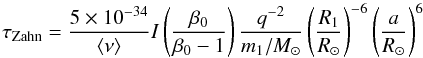 (35)where
τZahn is in seconds.
(35)where
τZahn is in seconds.
In order to compare our synchronization times obtained from Eq. (33) with those predicted in Eq. (35), we now make the simplifying assumption of
uniform density, from which  .
.
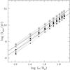 |
Fig. 7 Synchronization time computed with Eq. (33) using the results given in Fig. 3. The meaning of symbols stays the same as in Fig. 3. The continuous lines are the theoretical result obtained by
using Eq. (2.5) from Zahn (2008), under the
assumption of a uniform density structure ( |

In Fig. 7 we show the values of τsyn obtained from our Ė values and Eq. (33). These results have approximately the predicted a6 dependence, as obtained in Toledano et al. (2007) with our earlier model. We also see that the derived synchronization times depend on stellar rotation, with the faster rotating stars (β0 = 2) attaining synchronization significantly faster than slower rotators (β = 1.2).
The two continuous lines are Zahn’s theoretical result given by Eq. (35) for the two values of
β0, using
m1 = 5 M⊙,
m2 = 4 M⊙,
R1 = 3.2 R⊙, and
⟨ ν ⟩ = 3.4 × 1012 cm2 s-1. Our
results are consistent with this theoretical result, except that the value we used for the
kinematical viscosity in the calculations is significantly higher,
 d-1 = 1.7 × 1014 cm2 s-1.
It is important to note that in our calculation the tidal friction comes from the shear at
the interface of each surface element with its neighbors and with the inner (rigidly
rotating) boundary. This means that the action of the kinematical viscosity is limited to
these shearing surfaces. In addition, because ours is a single-layer approximation, there
is no buoyancy, and therefore our viscosity values are not associated with convection, as
are those of Zahn (1977, 2008). Hence, at this stage, we are only able to draw an equivalence
between the viscosity parameter used in our model and that used in Zahn’s formalism
through the comparison of the synchronization timescales, as shown in Fig. 7. That
⟨ ν ⟩ ~ 10-2ν is likely because
in our calculations the whole energy dissipation is forced to occur in the surface layer,
whereas in Zahn’s formalism deeper layers are also involved in these processes.
d-1 = 1.7 × 1014 cm2 s-1.
It is important to note that in our calculation the tidal friction comes from the shear at
the interface of each surface element with its neighbors and with the inner (rigidly
rotating) boundary. This means that the action of the kinematical viscosity is limited to
these shearing surfaces. In addition, because ours is a single-layer approximation, there
is no buoyancy, and therefore our viscosity values are not associated with convection, as
are those of Zahn (1977, 2008). Hence, at this stage, we are only able to draw an equivalence
between the viscosity parameter used in our model and that used in Zahn’s formalism
through the comparison of the synchronization timescales, as shown in Fig. 7. That
⟨ ν ⟩ ~ 10-2ν is likely because
in our calculations the whole energy dissipation is forced to occur in the surface layer,
whereas in Zahn’s formalism deeper layers are also involved in these processes.
4.2. Eccentric orbits
Equation (33) can be conveniently
written13 for an eccentric orbit in terms of the
synchronicity parameter at periastron, β0 and the orbital
eccentricity e, as  (36)where
m1 and R1 are the primary star’s
mass and radius, respectively, in solar units, and P is the orbital
period in days. The synchronization times obtained with the above equation, using the
Ėave values that are plotted in Fig. 4 are shown in Fig. 8. Several
features of this plot are notable: 1) there is a clear difference between moderately
eccentric (e ≲ 0.3) and the very eccentric systems; 2) at large orbital
separations (a ≥ 100 R⊙), the slope
significanlty flattens from the
τsyn ~ (a/R⊙)6
that applies for circular orbits14; and 3) for a
fixed value of a, the timescale for synchronization of the eccentric
binaries is shorter than the corresponding circular orbit binary, with differences as
large as five orders of magnitude visible in Fig. 8.
(36)where
m1 and R1 are the primary star’s
mass and radius, respectively, in solar units, and P is the orbital
period in days. The synchronization times obtained with the above equation, using the
Ėave values that are plotted in Fig. 4 are shown in Fig. 8. Several
features of this plot are notable: 1) there is a clear difference between moderately
eccentric (e ≲ 0.3) and the very eccentric systems; 2) at large orbital
separations (a ≥ 100 R⊙), the slope
significanlty flattens from the
τsyn ~ (a/R⊙)6
that applies for circular orbits14; and 3) for a
fixed value of a, the timescale for synchronization of the eccentric
binaries is shorter than the corresponding circular orbit binary, with differences as
large as five orders of magnitude visible in Fig. 8.
 |
Fig. 8 Synchronization from the energy dissipation rates computed with our model using a
kinematical viscosity |
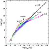 |
Fig. 9 Same synchronization times in the previous figure, but here plotted as a function of periastron distance, rper. The dotted lines connect the points corresponding to each of the eccentricities. τsyn is in units of years. |
The separation into these different “families” is eliminated in part by using the periastron distance, rper, instead of the semi-major axis of the orbit. Figure 9 illustrates the same values of Ė shown in Fig. 8, but in this case τsyn is plotted as a function of rper. The different curves “collapse” onto a common region in the log (τsyn) vs. log (rper) plane, with significant differences occuring only for very large orbital separations. This is consistent with the fact that, although the mean distance between the two stars increases with e, the distance at periastron strongly decreases, and as emphasized by Leconte et al. (2010), most of the work caused by tidal forces occurs at this point of the orbit.
The actual values of τsyn depend on the values of ν and k. But the scaling of τsyn with separation at periastron is as plotted in Fig. 8, unless ν and k depend on orbital separation15.
5. Orbital phase-dependence and periastron events
Consider the binary system with e = 0.8 and P = 15 d from the grid of models described in the previous sections. With β0 = 1.2, the primary star, m1, is rotating at 193 km s-1. The maps in the top panels of Fig. 10 are a color-coded Mollweide projection of the stellar surface, with white corresponding to the maximum elevation from the unperturbed stellar surface and black to the largest depression below the unperturbed stellar surface. Azimuth angle ϕ = 0°, corresponding to the location of m2, is on the left edge of the map, ϕ = 360° on the right edge, and ϕ = 180° is at the center. At periastron (Fig. 10, left), the surface acquires a shape that is typical of that assumed in the “equilibrium tide” approximation. That is, a tidal bulge is raised on both hemispheres with the larger bulge pointing in the general direction of the companion, m2, but “lagging" slightly behind. The maximum height of the primary bulge at the equator (Fig. 10, bottom left) is ~ 0.03 R⊙16.
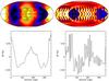 |
Fig. 10 Top: maps of radius residuals (r(ϕ′) − R1) for e = 0.8, P = 15 d, β0 = 1.2 at periastron (left) and 0.833 days after (right). The sub-binary longitude (ϕ′ = 0) is at the far left on each map and ϕ′ = 180° is at the center. The sense of the stellar rotation is from left-to-right. White/black represents maximum/minimum residuals. Bottom: corresponding plots of the radius residuals along the equator. |
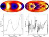 |
Fig. 11 Top: maps of tangential velocity residuals for e = 0.8, P = 15 d, β0 = 1.2 at periastron (left) and 0.833 days after (right). The sub-binary longitude (ϕ′ = 0) is at the far left on each map and ϕ′ = 180° is at the center. The sense of the stellar rotation is from left-to-right. White/black represents positive/negative residuals; i.e., particles moving faster/slower than the unperturbed stellar rotation velocity. Bottom: corresponding plots along the equator. |
The “equilibrium tide” configuration does not subsist very long, however. The right-hand panel of Fig. 10 illustrates the deformations just 0.833 day after periastron, and clearly the “equilibrium tide” approximation no longer represents the stellar surface shape. Now it is best described in terms of a large number of smaller-scale spatial structures. These would fall into the “dynamical tide” representation, if they were associated with the normal modes of oscillation of the stellar interior17. The amplitude of these structures declines with orbital phase as apastron is approached. A more in-depth analysis of the smaller spatial structures and their dependence on the model input parameters goes beyond the scope of the current paper, but the important point to note is that the “equilibrium tide” approximation is valid only around periastron passage for this particular highly eccentric model binary case. We find that for systems in our computed grid with low eccentricities and/or large orbital periods, the approximation remains valid over the orbital cycle, but not in the more extreme cases. However, even there, the tidal bulges raised by the secondary cannot be assumed to be steady over the orbital cycle, neither in amplitude nor in location.
We illustrate the azimuthal velocity field,
vϕ′, in Fig. 11. The explanation given by Tassoul (1987)
in the context of circular orbits is most appropriate to describe the phenomenon displayed
at periastron (left): “Assume that at some initial instant the primary is rotating rigidly
with a constant supersynchronous angular velocity. If there were no companion, the system
would remain forever axisymmetric. Because of the presence of the secondary, however, a
fluid particle moving on the free surface of the primary will experience small accelerations
and decelerations in the azimuthal direction. Hence, in the sectors
0° < ϕ′ < π/2 and
π < ϕ′ < 3π/2, the
azimuthal component  , of this fluid
particle will be smaller than the typical value by a small amount. On the contrary, in the
other sectors, will be
larger”. Note that in the case shown in Fig. 11 the
pattern of positive and negative residuals is slightly rotated with respect to Tassoul’s
description because this is not a circular-orbit case, and also because of the “lag” of the
primary tidal bulge. This quadrupolar pattern rapidly breaks down into smaller scale
structures after periastron, corresponding to the smaller spatial structures of Fig. 10 (right).
, of this fluid
particle will be smaller than the typical value by a small amount. On the contrary, in the
other sectors, will be
larger”. Note that in the case shown in Fig. 11 the
pattern of positive and negative residuals is slightly rotated with respect to Tassoul’s
description because this is not a circular-orbit case, and also because of the “lag” of the
primary tidal bulge. This quadrupolar pattern rapidly breaks down into smaller scale
structures after periastron, corresponding to the smaller spatial structures of Fig. 10 (right).
 |
Fig. 12 Top: maps of energy dissipation rate for e = 0.8, P = 15 d, β0 = 1.2 at periastron (left) and 0.833 days after (right). The sub-binary longitude (ϕ′ = 0) is at the far left on each map and ϕ′ = 180° is at the center. The sense of the stellar rotation is from left-to-right. White/black represents maximum/minimum residuals. Bottom: corresponding plots along the equator. |
Highest energy dissipation rates are associated with the regions having large perturbations in the azimuthal motion, both positive and negative. At periastron (Fig. 12, left), the highest Ė values occur close to the sub-binary longitude. But by 0.833 day later (Fig. 12, right), the large regions where most of the Ė was generated have broken down into small spatial scale structures. It is noteworthy, however, that some of these smaller structures are associated with significantly high values of Ė. Also noteworthy is that nearly the entire Ė occurs at ± 45° from the equatorial latitude.
The main conclusions we draw from this example are that 1) periastron passage causes a sudden and brief change in the surface perturbations, leading to significant dynamical effects; 2) the tidal shear energy dissipation rates are concentrated (in this example) around the equatorial latitude. Hence, the question arises as to whether these phenomena may provide a natural explanation for the periastron events described in the introduction, as well as the creation of a disk from the ejected material. The topic of how the material may be ejected goes beyond the scope of this paper18, but a plausible scenario is that additional energy is fed into sub-photospheric layers by the tidal shear, combined with the possible additional turbulence caused by the rapidly-changing motions on the stellar surface. We suggest that one of the crucial ingredients is the extremely rapid and strong forcing to which the stellar surface is subjected during periastron passage in very eccentric systems. Figure 13 shows a plot of Ė as a function of orbital phase for the e = 0.8, P = 15 d binary model discussed above and two other cases for comparison.19 The rapid rise in the Ė value at periastron is evident.
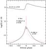 |
Fig. 13 Tidal shear energy dissipation rate for very eccentric binary systems as a function of orbital phase measured from periastron passage. Ė is in erg s-1 and ρ in g cm-3. Shown in this figure are two cases with e = 0.8 (P = 15 and 350 days) and a case for δ Sco. Note that peristron passage is always associated with a very large time variation of Ė. |
The second case depicted in Fig. 13 corresponds to a e = 0.8, P = 350 d model from our grid, and the unperturbed equatorial rotation velocity of m1 is ~8 km s-1. The Ė values undergo a ~6 order-of-magnitude variation between apastron and periastron, most of which occurs within ± 70 days of periastron passage. Finally, the third case illustrated in Fig. 13 is an exploratory model calculation for the extremely eccentric (e = 0.94) Be-type binary system δ Sco20. The primary star in this system has an estimated equatorial rotation velocity of ~200 km s-1, which means that it is rotating extremely fast, compared to the orbital angular velocity of m2. The star undergoes an increase in Ė by ~9 orders of magnitude between apastron and periastron, with a very steep rise to maximum just 15 days before periastron.
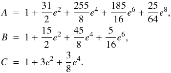
6. Discussion
A large body of research, starting with Darwin (1880), exists on the effects produced by tidal interactions on the long-term evolution of binary systems. The primary concern of these investigations is generally the timescales for circularization of the orbit and synchronization of the rotational and orbital angular velocities. The three general approaches that have been developed for analyzing the effect of tidal dissipation in these investigations are 1) the “equilibrium tide” model; 2) the “dynamical tide” model; and 3) the hydrodynamical model of Tassoul (1987).
In the “equilibrium tide” model (Darwin 1880; Alexander 1973; Hut 1980, 1981; and see Eggleton et al. 1998, and references therein)21 the shape of the stellar surface is approximated to that which it would adopt in equilibrium under the effect of the gravitational-centrifugal potential of the system. The viscous nature of the stellar material leads to a misalignment (refereed to as “lag”) between the axis that connects the two tidal bulges and the line that connects the centers of the two stars. The action of the external gravitational field on this misaligned body leads to a torque which, in turn, leads to an interchange of energy and angular momentum between stellar rotation and orbital motion. Dissipation by viscosity results in the decrease in the eccentricity of the orbit and the synchronization of the rotational and orbital motions. It is important to note that the “equilibrium tide” approach implicitly assumes that the star goes through a succession of rigidly rotating states, until the equilibrium configuration is reached.
The “dynamical tide” approach is based on the assumption that the star may be viewed as an oscillator whose normal modes may be excited by the variation in the gravitational potential. Among the first mathematical formulations available in the published literature are those of Fabian et al. (1975), Zahn (1975), and Press & Teukolsky (1977). In more recent years, a large amount of effort has been invested in further developing these concepts, as reviewed by Savonije (2008) (see, also McMillan et al. 1987; Goldreich & Nicholson 1989; Dolginov & Smel’Chakova 1992; Lai 1996; Mardling 1995; Kumar & Goodman 1996; Kumar & Quataert 1997). Three types of modes are believed to be excited a) the internal gravity modes, where the restoring force is the bouyancy force in stably stratified regions (Zahn 1975, 1977; Goldreich & Nicholson 1989; Rocca 1989); b) the acoustic modes, where the restoring force is the compressibility of the gas; and c) the inertial modes where the restoring force is the Coriolis force (Witte & Savonije 1999a,b). These modes are the mechanism by which energy from the orbital motion is absorbed by the star. The system is driven toward the equilibrium state by the damping of these modes. Hence, it is necessary to make an assumption concerning the damping mechanism. In stars with an outer convective layer, it is generally assumed that turbulent viscosity is the dominant mechanism. In stars with outer radiative layers, radiation damping is assumed to be the dissipative mechanism. It is interesting that in an eccentric system, the gravitational forcing goes through a large range of frequencies as the orbit progresses from apastron to periastron. Hence, there is a good chance that one of these frequencies will resonate with the star’s normal modes, thus exciting the particular oscillation mode in the star. At the same time, as periastron is approached, however, the star becomes more deformed, thus potentially modifying its normal modes. The above methods rely on a mathematical formulation of the star’s response to the perturbing potential of its companion, and are usually treated in the linear regime. Thus, they are generally limited to slow rotational velocities and/or low orbital eccentricites.
The third approach, introduced by Tassoul (1987) for early-type binaries, involves large-scale hydrodynamical motions within the tidally distorted star. It is based on the assumed presence of large-scale meriodional circulation, superposed on the mean azimuthal motion of stellar rotation. This circulation is believed to arise because a fluid particle moving on the free surface of the primary will experience small accelerations and decelerations in the azimuthal direction, depending on its location with regard to the sub-binary longitude22. These meridional circulation currents transport angular momentum very efficiently, which leads to very rapid synchronization timescales; i.e., the spin-down time primarily depends on (a/R)4.125. This mechanism is thus a more long-range mechanism compared with the other two. The method recognizes that near the surface, the Coriolis force and the viscous force must play a donominant role in the mechanical balance. Hence, this approach significantly differs from the other two in that it captures the hydrodynamic processes near the stellar surface.
Contrary to the three methods described above, where the primary concern is the long-term ( ≥ 106 yr) evolution of the orbital and stellar rotation parameters, our method was developed to analyze the tidal effects on orbital timescales (~days). However, we are able to compare the results of our model with results from the other models through the energy dissipation rates which, in turn, allow an estimate to be made of the synchronization timescales. We find that the results of our model for circular orbits are fully consistent with the results of Zahn (1977, 2008) for stars with convective envelopes. We also find that for eccentric orbits, our results for the scaling of the energy dissipation rates with orbital eccentricity and separation are consistent with the predictions of Hut (1981).
Zahn’s synchronization timescale for convective envelopes is based on the “dynamical tide” formalism, while Hut’s method is based on the “equilibrium tide” approximation. Our method does not rely on any a priori assumption regarding the mathematical formulation of the tidal flow structure. Instead, we solve the equations of motion of a thin, deformable surface layer that is allowed to respond to the gravitational field of m1 and m2, the Coriolis force, the centrifugal force, the gas pressure and the viscous forces from the shearing flows. The numerical solution of this system of equations yields the velocity field on the stellar surface, from which the energy dissipation rates may be computed. Thus, ours is a computation from first principles, the only simplifying assumptions being those which are inherent to the one-layer approximation. In particular, our method neglects the deformations produced by the tidal effects on the layers below the surface layer. However, because the tidal forces decline as 1/r3, the tidal effects are weaker in deeper layers of the star than on the surface (see, for example, Dolginov & Smelch’akova 1992). On the other hand, we are fully aware that the detailed behavior of underlying layers will be coupled to that of the surface layer. Thus, at this stage our results are merely indicative of the detailed behavior of the surface layer as a function of the orbital phase.
Among the advantages of our method is that it allows a qualitative assessment of the response of the stellar surface under arbitrary conditions and it captures the essence of the three general approaches described above. That is, the solution of the equations of motion yields a first-order deformation attributable to the equilibrium tide and a lag angle; a second order deformation attributable to dynamical effects23; and because of the inclusion of gas pressure, it captures some of the hydrodynamical effects. Interestingly, our results for the synchronization timescales in eccentric orbits are consistent with the equilibrium tide approach at intermediate orbital separations, but suggest much faster synchronization timescales for larger orbital separations, consistent with Tassoul’s hydrodynamic model24. From the observational standpoint, Abt & Boonyarak (2004) found that B and A stars in binaries with periods as long as 500 days have rotational periods significantly shorter than the corresponding single stars. They therefore concluded that the synchronization process can have an inpact on the stellar rotation even for relatively wide binaries with periods as long as 500 days, thus supporting the presence of a longer-range mechanism. Claret et al. (1995) and Claret & Cunha (1997) also have noted that the Zahn models and the Tassoul models each can explain the observational data only in part.
The major limitation of a one-layer model lies in neglecting the oscillatory nature of the stellar interior. In particular, the interaction of the normal modes of oscillation of the star with the external forcing frequency provides a means by which orbital energy might be captured by the star and deposited as thermal energy. Hence, we cannot at this time probe interesting situations associated with resonances. On the other hand, in long-period, very eccentric binary systems the peristron passage involves very large temporal gradients in the surface properties of the star. The tidal shear energy dissipation rates, in particular, change dramatically over a very small portion of the orbital cycle. Our exploratory calculation for the δ Sco binary system (orbital period P = 3944.7 days) indicates that Ė changes by five orders of magnitude over the 82 days before periastron, two of these occurring over the 15 days before peristron. The combination of added energy, extended radius, and high surface flow velocities may be envisaged to produce a destabilizing effect that leads to a mass-ejection event. Interestingly, we expect that the ejecta should form a disk-like structure, because the strongest tidal effects occur in the equatorial plane. Observational evidence for such a disk-forming event actually exists for the previous orbital cycle (Miroshnichenko et al. 2003). Confirming this behavior in the upcoming periastron passage of 2011 would strengthen the hypothesis.
Finally, we note that it may be productive to use the periastron distance, rper, instead of the semi-major axis, a, when comparing statistical studies of observational properties with theoretical models of tidal evolution. We show that by using rper, the synchronization timescales for binaries with different orbital eccentricities “collapse” into a small region in the τsyn vs. rper diagram, whereas on the τsyn vs. a diagram, there is a different “family” of curves corresponding to each eccentricity. This means that for a fixed value of a, the synchronization timescale derived from eccentric binary systems is significantly shorter (by orders of magnitude) than a corresponding e = 0 system. However, if rper is used instead, the spread between systems with different eccentricites is smaller.
We emphasize moreover that there is a significant dependence of τsyn on the stellar rotational velocity. However, it must be kept in mind that the important parameter is not only the equatorial rotational velocity, but also the synchronicity parameter, β0. Hence, slowly rotating stars may undergo strong tidal interaction effects if, for example, β0 ≪ 1. Whether strong tidal effects can contribute to alter chemical abundances is a question that merits examination, because this could potentially be an explanation for some of the discrepancies recently found between stellar structure evolutionary models and observations (Hunter et al. 2008; Brott et al. 2011).
Clearly, many of the outstanding questions associated with tidal interactions require a more complete treatment than that of any of the currently developed models. In particular, the departures from spherical symmetry imply that a one-dimensional treatment of the radiative transfer processes is inadequate. Furthermore, the energy that is dissipated due to tidal interactions, regardless of the mechanism invoked, is an added source of energy that is deposited in sub-photospheric layers of the star and needs to be considered when analyzing energy transport processes and determining the structure of the outer stellar layers.
7. Conclusions
We derived a mathematical expression for computing the rate of dissipation, Ė, of kinetic energy by the viscous flows that are driven by tidal interactions and used it to explore the effects caused by periastron passage in eccentric binary systems. Our method does not rely on any a priori assumptions regarding the mathematical formulation for the perturbations in the star caused by its companion. We show that our results for the scaling of Ė with orbital separation for circular orbits are the same as those derived analytically by Hut (1981), and that our results yield the same scaling of synchronization timescales with orbital separation as found by Zahn (1977, 2008) for convective envelopes. For elliptical orbits, our results reproduce the dependence of Ė on the eccentricity and the general trend with orbital separation as predicted by Hut (1981). In addition, the model also adequately predicts the pseudo-synchronization angular velocity for moderate eccentricities (e ≤ 0.3), as obtained by Hut (1981).
We explored the distribution of Ė over the stellar surface, and found that its configuration in small eccentricity binaries is consistent with the quadrupolar morphology of the “equilibrium tide”. That is, maximum Ė values tend to be located at four longitude regions where the fastest azimuthal motions are present. In very eccentric systems, however, the morphology significantly changes as a function of orbital phase. Although generally quadrupolar-like at periastron, shortly after this time Ė is distributed into smaller spatial structures, which suggests an analogy with the “dynamical tide” models. In addition, the perturbations are in general strongest around the equatorial latitude25.
We speculate that the very large and sudden increase in Ė that occurs around periastron, combined with the rapid growth rate of the velocity perturbations is a promising mechanism for explaining the increased stellar activity and mass-ejection events often observed around this orbital phase. Two factors may be involved in causing the periastron events. First, Ė is an additional source of energy that is deposited in sub-photospheric layers and represents a time-dependent perturbation to the temperature and differential velocity structure of these layers.
Second, in very eccentric binaries, the growth rate of the surface perturbations increases very abruptly at periastron. For example, in the very eccentric binary system δ Sco (e = 0.94, P = 3944.7 d), our exploratory calculation indicates that Ė changes by five orders of magnitude over the 82 days before periastron, with a two-orders of magnitude increase over the 15 days before peristron. The qualitative phenomenon is one in which portions of the stellar surface are forced to suddenly rotate faster or slower than their neighboring inner layers, thus leading to a variable differentially-rotating structure which significantly differs from its unperturbed structure. Furthermore, most of the activity occurs around the equatorial latitude. The consequence for the stability of the outer layers under these conditions is a problem that merits further attention.
A binary star is defined to be in equilibrium (Hut 1980) when it is in a circular orbit (e = 0), its rate of equatorial rotation equals the rate of orbital motion (ωrot = Ω) and the axes of stellar and orbital angular velocity are both perpendicular to the orbital plane.
Equations (40b) and (40c) given in Scharlemann (1981) indicate that for a colatitude angle θ > 70°, the maximum perturbation in the azimuthal direction is more than 15 times greater than the maximum perturbation in the polar direction.
The expression
βper = ω0/Ωper = 0.02 P  is a convenient form to compute the synchronicity parameter at periastron. P
is in days, vrot in km s-1, and
R1 in R⊙.
is a convenient form to compute the synchronicity parameter at periastron. P
is in days, vrot in km s-1, and
R1 in R⊙.
The Binary Evolutionary Code, Langer (1991).
m1 = 5 M⊙, with an age of 4.29125 × 10⁷ yrs, at which time its radius is 3.156 R⊙.
Appendix A shows the manner in which the Ė results depend on the chosen depth of the surface layer.
The model has recently been revisited by Leconte et al. (2010) in the context of tidal heating in exoplanets. These authors extended Hut’s equations to the case in which the orbital plane and the rotational equatorial plane of the objects do not coincide. A similar extension was also given in Eggleton et al. (1998).
An example of the orbital-phase dependence of α computed with our model may be found in Koenigsberger et al. (2003).
We note that at periastron, α is indeed very small (see, for example, Fig. 10), but grows after periastron passage.
Recall that in circular orbits, equilibrium configuration is at β0 = ω/Ω0 = 1, where Ė = 0.
For the fixed value of ν chosen for these calculations, very high stellar rotation rates cause neighboring surface elements to overlap, a condition which halts the computation.
Note, however, as shown by Hut (1981), the lowest energy state for the eccentric system corresponds to the pseudosynchronization period which, for moderate eccentricities, is β ~ 0.8–0.9.
Using Ω0 = 1.428 × 10⁻⁴vrot/R1β0, and vrot = β0R1(1 + e)1/2/ [0.02P(1 − e)3/2], where vrot is in km s-1, P is in days, and R1 in R⊙.
Note that for a ≥ 100 R⊙, τsyn ~ (a/R⊙)4.125, similar to the synchronization timescale predicted by Tassoul (1987).
Because ν is generally associated with turbulence, and because the perturbations of the surface velocity field in short-period binaries is very strong, the turbulent component in these systems may be much stronger than in wider binary systems. Thus, the use of a constant viscosity for all orbital separations may not be the most appropriate.
A rough estimate (cf., Zahn 2008) of the tidal bulge elevation for a non-rotating star with similar characteristics, δR/R1 ~ (m1/m2)(R1/rper)4 ~ 0.02, thus predicting δR = 0.07 R⊙, a factor 2.5 larger than predicted by our model.
Recall that the stellar interior here is a rotating, rigid body.
See, for example, Lee (1993).
Note that actual binary systems with this eccentricity and orbital period are extremely rare or non-existent, as can be seen in Fig. 1 of Mazeh (2008), which is probably because of the very large Ė, which should rapidly tend to circularize the orbit.
The parameters used for this calculation are m1 = 15 M⊙, m2 = 2 M⊙, P = 3944.7 d, R1 = 7 R⊙, β0 = 28.5, ΔR1/R1 = 0.06, β0 = 28.5, ν = 0.08 R2⊙ d-1.
An illustrative description and discussion of the limitations of this model may be found in Ferraz-Mello et al. (2008).
Indeed, our simulations show that these azimuthal motions are the dominant cause of photospheric line-profile variability on orbital timescales (Harrington et al. 2009).
Clearly, the dynamical effects predicted by the model refer to the surface layer only.
Note, however, that our model does not currently include meridional motions. The connection with the Tassoul model resides in the concept of the azimuthal flow velocities. These have significantly faster speeds than those of meridional flows and act on very short timescales.
The equator coincides with the orbital plane in our models.
Acknowledgments
We express our gratitude to Frederic Masset for a critical reading of this paper and very helpful suggestions, and to the referee, Peter Eggleton, for important comments. We also thank J. Kuhn, P. Garaud, and A. Maeder for motivating and helpful discussions; I. Brott for the 5 M⊙ stellar model; and Alfredo Díaz and Ulises Amaya for computing assistance. This research was funded under grants DGAPA/PAPIIT/UNAM 106708; CONACYT 48929; travel support to GK and DMH from the CONACYT-NSF collaborative program is acknowledged.
References
- Abt, H. A., & Boonyarak, C. 2004, ApJ, 616, 562 [Google Scholar]
- Alexander, M. E. 1973, A&ASS, 23, 459 [Google Scholar]
- Bedding, T. R. 1993, AJ, 106, 768 [Google Scholar]
- Bonacić Marinović, A. A., Glebbeek, E., & Pols, O. R. 2008, A&A, 480, 797 [NASA ADS] [CrossRef] [EDP Sciences] [Google Scholar]
- Brott, I., Langer, N., de Koter, A., et al. 2011, A&A, in press [Google Scholar]
- Claret, A., & Cunha, N. C. S. 1997, A&A, 318, 187 [NASA ADS] [Google Scholar]
- Claret, A., Giménez, A., & Cunha, N. C. S. 1995, A&A, 299, 724 [NASA ADS] [Google Scholar]
- Darwin, G. H. 1880, Philos. Trans. R. Soc. London, 171, 713 [NASA ADS] [CrossRef] [Google Scholar]
- Dolginov, A. Z., & Smelch’akova, E. V. 1992, A&A, 257, 783 [NASA ADS] [Google Scholar]
- Efroimsky, M., & Williams, J. G. 2009, Celestial Mechanics and Dynamical Astronomy, 104, 257 [Google Scholar]
- Eggleton, P. P., Kiseleva, L. G., & Hut, P. 1998, ApJ, 499, 853 [NASA ADS] [CrossRef] [Google Scholar]
- Fabian, A. C., Pringle, J. E., & Reese, M. J. 1975, MNRAS, 172, 15 [NASA ADS] [CrossRef] [Google Scholar]
- Fehlberg, E. 1968, NASA TR R-287 [Google Scholar]
- Ferraz-Mello, S., Rodtríguez, A., & Hussmann, H. 2008, Celestial Mechanics and Dynamical Astronomy, 101, 171 [NASA ADS] [CrossRef] [Google Scholar]
- Goldreich, P., & Nicholson, P. D. 1989, ApJ, 342, 1079 [NASA ADS] [CrossRef] [Google Scholar]
- Harrington, D., Koenigsberger, G., Moreno, E., & Kuhn, J. 2009, ApJ, 704, 813 [NASA ADS] [CrossRef] [Google Scholar]
- Hunter, I., Brott, I., Lennon, D. J., et al. 2008, ApJ, 676, L29 [NASA ADS] [CrossRef] [Google Scholar]
- Hut, P. 1980, A&A, 97, 167 [NASA ADS] [Google Scholar]
- Hut, P. 1981, A&A, 99, 126 [NASA ADS] [Google Scholar]
- Koenigsberger, G., & Moreno, E. 1997, in Luminous Blue Variables: Massive Stars in Transition, ed. A. Nota, & H. Lamers, ASP Conf. Ser., 120, 233 [Google Scholar]
- Koenigsberger, G., & Moreno, E. 2008, Rev. Mex. Astron. Astrofis. (SC), 33, 108 [Google Scholar]
- Koenigsberger, G., Moreno, E., & Cervantes, F. 2002, Interacting winds from Massive Stars, ed. A. F. J. Moffat, & N. St-Louis, ASPCS, 260, 507 [Google Scholar]
- Koenigsberger, G., Moreno, E., & Cervantes, F. 2003, A massive star Odyssey, from Main Sequence to Supernova, ed. K. A. van der Hucht, A. Herrero, & C. Esteban, Proc. IAU Symp., 212, 101 [Google Scholar]
- Koenigsberger, G., Georgiev, L., Moreno, E., et al. 2006, A&A, 458, 513 [NASA ADS] [CrossRef] [EDP Sciences] [Google Scholar]
- Kumar, P., & Quataert E. J. 1997, ApJ, 479, L51 [NASA ADS] [CrossRef] [Google Scholar]
- Kumar, P., & Goodman, J. 1996, ApJ, 466, 946 [NASA ADS] [CrossRef] [Google Scholar]
- Lai, D. 1996, ApJ, 466, L35 [NASA ADS] [CrossRef] [Google Scholar]
- Langer, N. 1991, A&A, 252, 669 [NASA ADS] [Google Scholar]
- Leconte, J., Chabrier, G., Baraffe, I., & Levrard, B. 2010, A&A, 516, A64 [NASA ADS] [CrossRef] [EDP Sciences] [Google Scholar]
- Lee, U. 1993, ApJ, 417, 697 [NASA ADS] [CrossRef] [Google Scholar]
- Lynden-Bell, D., & Pringle, J. E. 1974, MNRAS, 168, 603 [NASA ADS] [CrossRef] [Google Scholar]
- Mardling, R. A. 1995, ApJ, 450, 732 [NASA ADS] [CrossRef] [Google Scholar]
- Mazeh, T. 2008, in Tidal Effects in Stars, Planets and Disks, ed. M.-J. Goupil, & J.-P. Zahn, EAS Pub. Ser., 29, 1 [Google Scholar]
- McMillan, S. L. W., McDermott, P. N., & Taam, R. E. 1987, ApJ, 318, 261 [NASA ADS] [CrossRef] [Google Scholar]
- McQuarrie, D. A. 1976, Statistical Mechanics (New York: Harper & Row) [Google Scholar]
- Millour, F., Chesneau, O., Borges Fernandes, M., et al. 2009, A&A, 507, 317 [NASA ADS] [CrossRef] [EDP Sciences] [Google Scholar]
- Miroshnichenko, A. S., Fabregat, J., Bjorkman, D. S., et al. 2001, A&A, 377, 485 [NASA ADS] [CrossRef] [EDP Sciences] [Google Scholar]
- Miroshnichenko, A. S., Bjorkman, K. S., Morrison, N. D., et al. 2003, A&A, 408, 305 [NASA ADS] [CrossRef] [EDP Sciences] [Google Scholar]
- Moreno, E., & Koenigsberger, G. 1999, Rev. Mex. Astron. Astrofis., 35, 157 [NASA ADS] [Google Scholar]
- Moreno, E., Koenigsberger, G., & Toledano, O. 2005, A&A, 437, 641 [NASA ADS] [CrossRef] [EDP Sciences] [Google Scholar]
- Press, W. H., & Teukolsky, S. A. 1977, ApJ, 213, 183 [NASA ADS] [CrossRef] [Google Scholar]
- Rocca, A. 1989, A&A, 213, 114 [NASA ADS] [Google Scholar]
- Savonije, G. 2008, in Tidal Effects in Stars, Planets and Disks, ed. M.-J. Goupil, & J.-P. Zahn, EAS Pub. Ser., 29, 91 [Google Scholar]
- Scharlemann, E. T. 1981, ApJ, 246, 292 [NASA ADS] [CrossRef] [Google Scholar]
- Symon, K. R. 1971, Mechanics (Addison-Wesley) [Google Scholar]
- Tango, W. J., Davis, J., Jacob, A. P., et al. 2009, MNRAS, 396, 842 [NASA ADS] [CrossRef] [Google Scholar]
- Tassoul, J. L. 1987, ApJ, 322, 856 [NASA ADS] [CrossRef] [Google Scholar]
- Toledano, O., Moreno, E., Koenigsberger, G., Detmers, R., & Langer, N. 2007, A&A, 461, 1057 [NASA ADS] [CrossRef] [EDP Sciences] [Google Scholar]
- van Genderen, & Sterken 2007, IBVS, 5782 [Google Scholar]
- Zahn, J. P. 1975, A&A, 41, 329 [NASA ADS] [Google Scholar]
- Zahn, J. P. 1977, A&A, 57, 383 [NASA ADS] [Google Scholar]
- Zahn, J. P. 2008, in Tidal Effects in Stars, Planets and Disks, ed. M.-J. Goupil, & J.-P. Zahn, EAS Pub. Ser., 29, 67 [Google Scholar]
Appendix A: Grid of model calculations
Summary of the 5 + 4 M⊙ model binary system models for
ΔR1/R1 = 0.06 and
 day-1
(unless noted otherwise).
day-1
(unless noted otherwise).
Table A.1 lists the input parameters of the grid
of model calculations used in this paper. The first column identifies the set number; the
second column lists the eccentricity; the third column lists the range in orbital periods
included in the given set; the fourth column lists the value of
β0 used in the calculation, or the range in
β0 values; and the last column contains comments. Unless
otherwise noted, all calculations were performed with a kinematical viscosity parameter,
 day-1 = 2.8 × 1014 cm2/s.
Appendix B: Dependence of Ėave on layer depth
We examined the manner in which the energy dissipation rates depend on the choice of the depth (ΔR1/R1) of the surface layer that is modeled. This was done holding all parameters fixed, except for the values of dR1/R1, which were varied from 0.02 to 0.10. The results for e = 0.1, 0.3 and 0.8 are illustrated in Fig. B.1, which show that for the models we have run for this paper, the calculations using different layer depths yield values of Ėave that differ by no more than a factor of two.
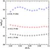 |
Fig. B.1 Dependence of Ėave on the choice of layer depth for models computed with e = 0.1, 0.3 and e = 0.8, and corresponding orbital periods as listed in the label. The average density for each layer depth used for the Ėave calculation were obtained from the stellar structure model of a 5 Mo, 3.15 Ro star (Brott 2010, private communication). This shows that for a fixed set of binary parameters, the energy dissipation rates depend on the choice of layer depth only within a factor of ~2. |
All Tables
Summary of the 5 + 4 M⊙ model binary system models for
ΔR1/R1 = 0.06 and
day-1
(unless noted otherwise).
All Figures
|
Fig. 1 Rate of energy dissipation Ėij as a
function of ϕ′ in a few selected parallels, for the
n = 1.5 polytropic case
ΔR1/R1 = 0.03,
ν = 0.003 |
| In the text | |
|
Fig. 2 Rate of energy dissipation in the parallel i as a function of its polar angle, corresponding to the computations in Fig. 1. Results with β0 = 1.2 and 2 are shown with empty and filled squares, respectively. The continuous lines show functions with a sin7θ′ dependence. |
| In the text | |
|
Fig. 3 Energy dissipation in m1 as a function of the separation a of the circular orbit. A polytropic index n = 1.5 is used. Empty symbols correspond to β0 = 1.2 and filled symbols to β0 = 2.0. The correspondence with the layer thickness ΔR1/R1 is, in triangles: ΔR1/R1 = 0.01, in squares: ΔR1/R1 = 0.03, in pentagons: ΔR1/R1 = 0.06. The continuous line is a function with an a-9 dependence on a. |
| In the text | |
|
Fig. 4 Energy dissipation rates (in erg s-1) from our model calculations for β0 = 1.2 and different eccentricities as indicated. The dashed lines show the absolute value of Ėorb given by Eq. (A31) of Hut (1981), as written in our Eq. (30). The dotted lines connect the points corresponding to each eccentricity. The short dot-dashed lines show the values of ĖHut for e = 0.8 and lag angles α = 10° and 50°. |
| In the text | |
|
Fig. 5 Energy dissipation rates of the previous figure but here plotted as a function of the periastron distance, rper. In this representation, the different curves for each eccentricity “collapse” onto a common region. The dashed lines show the absolute value of Ėorb given by Eq. (A31) of Hut (1981) for e = 0.1 and 0.8, also plotted as a function of rper. Symbols correspond to the different eccentricities: e = 0.00 (open triangles), 0.01 (filled triangles), 0.10 (small pentagons), 0.30 (large pentagons), 0.50 (crosses), 0.70 (stars) and 0.8 (filled pentagons). |
| In the text | |
|
Fig. 6 Energy dissipation rates Ėave/1035 ⟨ ρ ⟩ as a function of β0 = ω/Ω0 for four different eccentricities, e = 0.1 (top left), 0.3 (top right), 0.5 (bottom left) and 0.8 (bottom right). The first three cases are for an orbital period P = 6 d and the last is for 20 d. The ordinate is in units of 1035 ⟨ ρ ⟩ erg s-1, where ⟨ ρ ⟩ is the average density. The dotted line indicates the level of minimum Ėave which, for e = 0.1 and 0.3 coincides with the analytical results of Hut (1981). |
| In the text | |
|
Fig. 7 Synchronization time computed with Eq. (33) using the results given in Fig. 3. The meaning of symbols stays the same as in Fig. 3. The continuous lines are the theoretical result obtained by
using Eq. (2.5) from Zahn (2008), under the
assumption of a uniform density structure ( |
| In the text | |
|
Fig. 8 Synchronization from the energy dissipation rates computed with our model using a
kinematical viscosity |
| In the text | |
|
Fig. 9 Same synchronization times in the previous figure, but here plotted as a function of periastron distance, rper. The dotted lines connect the points corresponding to each of the eccentricities. τsyn is in units of years. |
| In the text | |
|
Fig. 10 Top: maps of radius residuals (r(ϕ′) − R1) for e = 0.8, P = 15 d, β0 = 1.2 at periastron (left) and 0.833 days after (right). The sub-binary longitude (ϕ′ = 0) is at the far left on each map and ϕ′ = 180° is at the center. The sense of the stellar rotation is from left-to-right. White/black represents maximum/minimum residuals. Bottom: corresponding plots of the radius residuals along the equator. |
| In the text | |
|
Fig. 11 Top: maps of tangential velocity residuals for e = 0.8, P = 15 d, β0 = 1.2 at periastron (left) and 0.833 days after (right). The sub-binary longitude (ϕ′ = 0) is at the far left on each map and ϕ′ = 180° is at the center. The sense of the stellar rotation is from left-to-right. White/black represents positive/negative residuals; i.e., particles moving faster/slower than the unperturbed stellar rotation velocity. Bottom: corresponding plots along the equator. |
| In the text | |
|
Fig. 12 Top: maps of energy dissipation rate for e = 0.8, P = 15 d, β0 = 1.2 at periastron (left) and 0.833 days after (right). The sub-binary longitude (ϕ′ = 0) is at the far left on each map and ϕ′ = 180° is at the center. The sense of the stellar rotation is from left-to-right. White/black represents maximum/minimum residuals. Bottom: corresponding plots along the equator. |
| In the text | |
|
Fig. 13 Tidal shear energy dissipation rate for very eccentric binary systems as a function of orbital phase measured from periastron passage. Ė is in erg s-1 and ρ in g cm-3. Shown in this figure are two cases with e = 0.8 (P = 15 and 350 days) and a case for δ Sco. Note that peristron passage is always associated with a very large time variation of Ė. |
| In the text | |
|
Fig. B.1 Dependence of Ėave on the choice of layer depth for models computed with e = 0.1, 0.3 and e = 0.8, and corresponding orbital periods as listed in the label. The average density for each layer depth used for the Ėave calculation were obtained from the stellar structure model of a 5 Mo, 3.15 Ro star (Brott 2010, private communication). This shows that for a fixed set of binary parameters, the energy dissipation rates depend on the choice of layer depth only within a factor of ~2. |
| In the text | |
Current usage metrics show cumulative count of Article Views (full-text article views including HTML views, PDF and ePub downloads, according to the available data) and Abstracts Views on Vision4Press platform.
Data correspond to usage on the plateform after 2015. The current usage metrics is available 48-96 hours after online publication and is updated daily on week days.
Initial download of the metrics may take a while.