| Issue |
A&A
Volume 528, April 2011
|
|
|---|---|---|
| Article Number | A28 | |
| Number of page(s) | 35 | |
| Section | Extragalactic astronomy | |
| DOI | https://doi.org/10.1051/0004-6361/201015719 | |
| Published online | 22 February 2011 | |
The WSRT Virgo Hi filament survey
II. Cross correlation data⋆
1
Laboratoire d’Astrophysique de Marseille,
38 rue Frédérique Joliot-Curie,
13388
Marseille Cedex 13,
France
e-mail: This email address is being protected from spambots. You need JavaScript enabled to view it.
2
Kapteyn Astronomical Institute, PO Box 800, 9700 AV
Groningen, The
Netherlands
3
CSIRO – Astronomy and Space Science, PO Box 76,
Epping,
NSW
1710,
Australia
Received: 8 September 2010
Accepted: 22 December 2010
Abstract
Context. The extended environment of galaxies contains a wealth of information about the formation and life cycle of galaxies which are regulated by accretion and feedback processes. Observations of neutral hydrogen are routinely used to image the high brightness disks of galaxies and to study their kinematics. Deeper observations will give more insight into the distribution of diffuse gas in the extended halo of the galaxies and the inter-galactic medium, where numerical simulations predict a cosmic web of extended structures and gaseous filaments.
Aims. To observe the extended environment of galaxies, column density sensitivities have to be achieved that probe the regime of Lyman limit systems. H i observations are typically limited to a brightness sensitivity of NHI ~ 1019 cm-2, but this must be improved upon by ~2 orders of magnitude.
Methods. In this paper we present the interferometric data of the Westerbork Virgo H i Filament Survey (WVFS) – the total power product of this survey has been published in an earlier paper. By observing at extreme hour angles, a filled aperture is simulated of 300 × 25 m in size, that has the typical collecting power and sensitivity of a single dish telescope, but the well defined bandpass characteristics of an interferometer. With the very good surface brightness sensitivity of the data, we hope to make new H i detections of diffuse systems with moderate angular resolution.
Results. The survey maps 135 degrees in Right Ascension between 8 and 17 h and 11 degrees in Declination between − 1 and 10 degrees, including the galaxy filament connecting the Local Group with the Virgo Cluster. Only positive declinations could be completely processed and analysed due to projection effects. A typical flux sensitivity of 6 mJy beam-1 over 16 km s-1 is achieved, that corresponds to a brightness sensitivity of NHI ~ 1018 cm-2. An unbiased search has been done with a high significance threshold as well a search with a lower significance limit but requiring an optical counterpart. In total, 199 objects have been detected, of which 17 are new H i detections.
Conclusions. By observing at extreme hour angles with the WSRT, a filled aperture can be simulated in projection, with a very good brightness sensitivity, comparable to that of a single dish telescope. Despite some technical challenges, the data provide valuable constraints on faint, circum-galactic H i features.
Key words: galaxies: formation / intergalactic medium
Appendix is only available at electronic form at http://www.aanda.org
© ESO, 2011
1. Introduction
In the current epoch, numerical simulations predict that most of the baryons are not in galaxies, but in extended gaseous filaments, forming a Cosmic Web (e.g. Davé et al. 1999; Cen & Ostriker 1999) Galaxies are just the brightest pearls in this web, as the baryons are almost equally distributed amongst three components: (1) galactic concentrations, (2) a warm-hot intergalactic medium (WHIM) and (3) a diffuse intergalactic medium. Direct detection of the intergalactic gas is very difficult at UV, EUV or X-ray wavelengths (Cen & Ostriker 1999) and so far the clearest detections have been made in absorption (e.g. Lehner et al. 2007; Tripp et al. 2008). In this and previous papers in this series, we make an effort to detect traces of the intergalactic medium in emission, using the 21-cm line of neutral hydrogen. Most of the gas in the Cosmic Web will be highly ionised, due to the moderately high temperatures above 104 K, resulting in a low neutral fraction and relatively low neutral column densities. A more detailed background and introduction on this topic is outlined in Popping (2010) and Popping & Braun (2011a)
To investigate column densities that probe the Lyman Limit System regime, very deep H i observations are required with a brightness sensitivity significantly better than NHI ~ 1019 cm-2. Reaching these column densities is important to learn more about the distribution of neutral hydrogen in the inter-galactic medium and to have a better understanding of feedback processes that fuel star formation in galaxies. In Popping & Braun (2011a) and Popping & Braun (2011b) two H i surveys have been presented that reach these low column densities in a region of ~1500 square degrees. The first data product described in Popping & Braun (2011a) is the total power data of the Westerbork Virgo Filament Survey, an H i survey mapping the galaxy filament connecting the Virgo Cluster with the Local Group. The survey spans 11 degrees in Declination from − 1 to +10 degrees and 135 degrees in Right Ascension between 8 and 17 h. This survey has a point source sensitivity of 16 mJy beam-1 over 16 km s-1 corresponding to a column density of NHI ~ 3.5 × 1016 cm-2.
The second data product presented in Popping & Braun (2011b) is reprocessed data, using original data that has been observed for the H i Parkes All Sky Survey (Barnes et al. 2001; Wong et al. 2006). The 1500 square degree region overlapping the WVFS was reprocessed to permit comparison between these data products and detections. The point source sensitivity of the reprocessed HIPASS data is 10 mJy beam-1 over 26 km s-1, corresponding to a column density of NHI ~ 3.5 × 1017 cm-2.
In this paper, a third data product is presented: the cross-correlation data of the Westerbork Virgo Filament Survey. As explained in Popping & Braun (2011a), the aim of the WVFS was to achieve very high brightness sensitivity in a large region of the sky, to permit detection of H i features that probe the neutral component of the Cosmic Web. The configuration of the array was chosen such that the dishes of the interferometer form a filled aperture of ~300 m in projection by observing at extreme hour angles. Because of the much smaller beam size compared to the WVFS total-power or HIPASS observations, we will be able to identify brighter clumps within diffuse features if these are present.
The special observing configuration creates some technical challenges itself. This novel observing strategy requires non-standard data-reduction procedures, which will be explained in Sect. 2. In Sect. 3 we will present the results, starting with a list of detected features. Objects are sought both blindly, by using a high signal-to-noise threshold, and in conjunction with a known optical counterpart by using a lower threshold. New H i detections and diffuse structures are briefly discussed, however detailed analysis of these features will be presented in a follow up paper, also discussing new and tentative detections obtained from the WVFS total-power data and the re-processed HIPASS data as described in Popping & Braun (2011a) and Popping & Braun (2011b). We will end with a short discussion and conclusion, summarizing the main results.
2. Observations and data reduction
The basic observations have already been described in Popping & Braun (2011a), where the total power product of the Westerbork Virgo Filament Survey is presented. Cross-correlation data were acquired simultaneously with that total power data. We will only summarise the observational parameters as these have been discussed previously and concentrate more on the observing technique and data reduction as these are very non-standard for this data set.
2.1. Observations
The galaxy filament connecting the Virgo Cluster with the Local Group has been observed using the Westerbork Synthesis Radio Telescope (WSRT) in drift scan mode. Data was acquired in two 20 MHz IF bands centred at 1416 and 1398 MHz. In total ~1500 degrees has been observed from −1 to 10 degrees in Declination and from 8 to 17 h in right ascension. Forty-five strips have been observed at fixed Declinations of Dec = −1, −0.75, −0.5 ... 10 degrees. The correlated data was averaged in Right Ascension every 60 s, corresponding to an angular drift of about 15 arcmin, to yield Nyquist sampling in the scan direction. All regions have been observed twice, once when the sources were rising and once when they were setting.
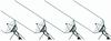 |
Fig. 1 Observing mode of the WSRT dishes: 12 of the 14 dishes are placed at a regular interval of 144 meters. When observing at large hour angles, an approximately filled aperture of 300 by 25 m can be simulated in projection. |
2.2. Observing technique
The data has been obtained at very extreme hour angles between ± 80 and ± 90 degrees, to be able to achieve a filled-aperture projected geometry. The WSRT has 14 dishes of 25 m diameter, of which 12 can be placed at regular intervals of 144 m. At these extreme hour angles, the dishes do not shadow each other, however the separation is so small that there are no gaps in the UV-plane. Using the 12 dishes at regular intervals, a filled aperture is created in projection of 300 × 25 m in extent as demonstrated in Fig. 1. When observing in this mode, we can achieve the high sensitivity of a single dish telescope, but benefit from the excellent spectral baseline properties and PSF of an interferometer. Although each pointing is only observed one minute at a time and two minutes in total, the expected sensitivity after one minute of observing is ΔNHI ~ 5 × 1017 cm-2 over 20 km s-1 in a ~35 × 3 arcmin beam over a ~35 × 35 arcmin instantaneous field-of-view. It is important to note that the shape of the beam in a single snap-shot is extremely elongated. The high column density sensitivity is only achieved in practise for sources which completely fill the beam, which is only likely for the nearest sources, or when they are fortuitously aligned with the elliptical beam. However, each pointing is observed at two complementary hour-angles; one positive and the other negative, implying that the orientation of the snap-shot beams is also complimentary. When combining the observations, the resulting beam has a well defined circular/elliptical shape, even though the orientation of each of the two beams is only a few degrees on either side of vertical. The concept is demonstrated in Fig. 2 where the combination of the individual elongated beams forms a symmetric, approximately circular response.
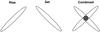 |
Fig. 2 Due to the filled aperture of ~300 × 25 meters, a very elongated beam is created. By observing each pointing twice at complementary orientations, the combined beam of the two observations is nearly circular, although with a significant side-lobe level. |
2.3. Data reduction
Both the auto and cross-correlation data have been obtained simultaneously, but were separated before importing them into Classic AIPS (Fomalont 1981). The reduction process of the auto-correlations or total power data has been described in detail in Popping & Braun (2011a). Here we will describe the cross-correlation data product.
A typical observation consisted of a calibrator source (3C 48 or 3C 286), the actual drift scan at a fixed Declination and another calibrator source. After importing the data into AIPS, the calibration and drift scan data were concatenated into a single file.
The total dataset consists of 90 drift-scans at fixed declination, containing 91 baselines in two polarisations; half observed at an extreme negative hour angle and the other half at an extreme positive hour angle. Each baseline was inspected manually in Classic AIPS, using the SPFLG utility. Suspicious features appearing in the frequency and time domain of each baseline were inspected critically. Features that were not confirmed in spectra acquired simultaneously were flagged as radio frequency interference (RFI).
Right ascension range and noise levels of the 18 individual sub-cubes of the WVFS cross-correlation data.
The calibrator sources were used to determine the bandpass calibration and the bandpass solutions were inspected by eye before application. Continuum data files were created from the line data by averaging the central 75% of the frequency bandwidth. These were used for determining the gain calibrations. As we are using the AIPS package which was originally developed for VLA data, a re-definition of the polarisation products is necessary for correct gain calibration. The VLA measures right and left circular polarisations (RR = I + V, LL = I − V, RL = Q + iU and LR = Q − iU), while the WSRT data consists of the two perpendicular linear polarisation products (XX = I − Q, YY = I + Q, XY = −U + iV and YX = −U − iV). Both definitions are in terms of the same true Stokes parameters (I, Q, U, V). By redefining a calibrator’s parameters as (I′, Q′, U′, V′) = (I, –U, V, –Q) it is possible to successfully calibrate the (XX,YY,XY and YX) data by treating it as if it were (RR,LL,RL and LR). Redefinition of polarization products has no effect for sources that are not polarised. However the calibrator, 3C 286, is known to be about 10% linearly polarised. The “apparent Stokes” values that have been used for this calibrator are (14.75, –1.27, 0, –0.56) Jy for the first IF and (14.83, –1.28, 0. –0.57) Jy for the second IF. Gain solutions determined with the continuum data are applied to the line data as well. The calibrated data is exported from AIPS into the uvfits format and imported into the Miriad (Sault et al. 1995) software package. Miriad has been used to further reduce the data. The mosaic scans are split into individual pointings. Continuum emission is subtracted from the line data using a first order polynomial, excluding the edge of the bandpass and regions containing galactic emission.
Although there are only scans at 45 different declinations, each scan contains 540 pointings in right ascension. Because the complete survey cannot be imaged simultaneously due to computer memory and image projection limitations, all the scans have been split into individual pointings. The complete survey is separated in 18 blocks of 40 pointings in right ascension and 45 pointings in declination, with a ten pointing overlap in right ascension between neighbouring blocks. This corresponds to sub-regions of ~10 × 11 degrees in size. The central positions of each of the sub-region cubes is listed in Table 1. When inverting the data from the UV to the image domain a uniform weighting scheme was applied, as this is the most optimal weighting for the 12 inner antennas of the array. Because of the regular antenna spacing, many baselines have the same length but the uv-plane is fully sampled at all spacings between one and eleven dish diameters. To suppress the side-lobes due to incomplete sampling of the longer baselines involving antennas 13 and 14, a Gaussian taper has been applied to the visibility data with a FWHM of 200 arcsec; as this is approximately the size of the final beam. The 250 individual velocity channels were imaged between 150 and 2000 km s-1 with a sampling of 8.24 km s-1. An example of a single channel in a sub-region is shown in Fig. 3, the inner 10 degrees in right ascension and declination have uniform mosaic sampling and an approximately constant noise level. Figure 4 shows the same field, overlaid with all the individual pointing patterns that have been used to mosaic this field.
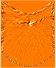 |
Fig. 3 Example of a channel map from one of the processed sub-region cubes (Cube 9) from the WVFS cross-correlation data. The inner region is well sampled by the pointings and the noise is uniform, while emission at the edges is noisier. There is 25% overlap in right ascension between adjacent cubes. Unfortunately the coordinates could not be shown in this plot due to projection effects, as explained in the text. |
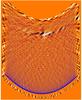 |
Fig. 4 Same image as Fig. 3, but now with the positions of the pointings overlaid. Each cube contains data from 45 pointings in declination, by 40 pointings in right ascension covering 11 by 10 degrees. Due to the NCP projection of the data, the declinations close to zero degrees are increasingly distorted, as can be seen in the shape of the pointings that are squeezed toward the lowest declinations. Unfortunately, pointings with both positive and negative declinations could not gridded simultaneously due to limitations of the NCP projection. |
Unfortunately the data from pointings with negative declinations are missing from the cubes, as well as the axis labels in the two plots that are shown. The data has been inverted using the Miriad software package, which grids and inverts the data using the natural NCP (North Celestial Pole) projection that applies to data obtained with an East-West interferometer. In most cases this is not a problem, however the NCP definition breaks down at a declination of zero degrees. The NCP projection is defined in Brouw (1971) by:  (1)and
  (2)At declinations approaching zero, the M-value diverges to infinity, making any projection impossible. The commonly used imaging tasks in both Miriad and AIPS have been found to work effectively when given either all positive or all negative declinations, but failed when given both simultaneously. Various methods of circumventing this problem have been tested, but none of them was successful in re-projecting all of the data to a more useful grid. We have therefore chosen to neglect the negative Declination pointings of the cross-correlation data, as they contain less than 10% percent of the total. Other projections for the northern part of the data have been considered, but these are not favorable since they yield a highly position dependant PSF. The data is gridded in NCP-projection, for which a well defined beam applies. When re-projecting the ~10 × 10 degree field to e.g. a SIN-projection, the response to point sources, particularly at the lowest declinations, is severely distorted. The effect of the NCP-projection can also be seen in the shape and distribution of the pointings in Fig. 4 as the pointings at low Declination are squeezed into narrow ellipses. Quite apart from the NCP-projection, it is an inherent property of an east-west interferometer, that the north-south spatial resolution that can be achieved at Dec = 0 is only as good as the primary beam, which is ~35 arcmin.
Figure 5 shows the synthesized beam for one of the central pointings in the strip at Dec = 10 degrees. The left panel shows the beam due to a single observation, which is extremely elongated. The right panel displays the beam after combining both complimentary observations. When averaging the two elongated beams, a circular main-lobe is formed, although substantial X-shaped side-lobes are also apparent.
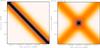 |
Fig. 5 Beam shape of a central pointing in the strip at Dec = 10 degrees. The left panel shows the synthesized beam of a single observation, while the right panel shows the beam for the combination of two complimentary scans. Both panels have the same intensity scale and contours are drawn at 70, 80 and 90 percent of the peak. |
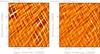 |
Fig. 6 The left panel shows a region of the dirty map; data that has only been inverted from the u,v plane to the image plane. The right panel shows exactly the same region after one pass of cleaning. While in the left panel the cross pattern of the beam is very apparent, in the right panel the side-lobes are almost completely subtracted. |
After the cubes have been imaged, the data were Hanning smoothed using a width of 3 channels, to eliminate spectral sidelobes and lower the rms noise. Although the channel sampling of the cubes is unchanged, the velocity resolution of the data is decreased to ~16 km s-1.
After Hanning smoothing has been applied, the beam and smoothed dirty maps were deconvolved using the MOSSDI task within Miriad to create clean cubes. This task is similar to the single-field CLEAN algorithm, but can be applied to mosaic-data. Only one pass of CLEAN deconvolution has been done without any masking. Because of the relatively large size of the 18 cubes, the cleaning step takes significant processing power. For the cleaning step a cutoff level of 50 mJy beam-1 was used. This cutoff level was determined empirically to be optimal in cleaning the data as deeply as possible while not creating false components. Although on the whole the data quality was significantly improved by deconvolution, the brightest sources are still suffering from some residual side-lobe artifacts. A second cleaning pass using a clean mask was not undertaken, since residual sidelobes prevented effective mask definition in an automatic way. The survey volume was deemed too large, to determine a mask manually. Nevertheless the improvement in dynamic range is significant as can be seen in the example shown in Fig. 6. In the left panel a channel is shown before cleaning and in the right panel the same field is shown after cleaning. In the left panel a very strong X-shaped sidelobe pattern can be seen at the location of bright sources. In the right panel the side-lobes have almost completely disappeared.
2.4. Sensitivity
We reach an almost uniform noise level throughout the survey area of 6 mJy beam-1 over 16 km s-1 which corresponds to a column density sensitivity of NHI ~ 1.1 × 1018 cm-2. The noise level in each of the individual 18 cubes is listed in Table 1. Although we reach very high sensitivities, we note that the data is affected by some residual side-lobe contamination in the vicinity of bright sources.
Typical features that occur in the data cubes are illustrated in Fig. 3. At the edge of the field there is an increase in the noise due to the finite number of mosaic pointings included in each cube. The large dark and light structure in the upper part of the field is caused by solar interference during the observation. This instance of solar interference is very extreme and certainly not typical. Distributed over the field are many galaxies that appear as point sources. The X-shaped residual side-lobe pattern is still apparent within the noise around the brightest of these sources in the field.
2.5. False positives
Although the reduced data has a good flux sensitivity, there are many artifacts in the data, that are important to understand. Because the “cleaning” step during the data reduction has not been perfect, there are artifacts in the vicinity of bright groups of sources that are caused by side-lobes in the beam. In some cases the residual side-lobes of a bright source are similar in strength to fainter sources in it’s vicinity.
At some locations, the quality of the data was not optimal and parts of several declination strips had to be flagged. As a result, the restoring beam is not well matched to the data at these locations and the sensitivity is  worse. Due to the extended nature of the mosaic pointing pattern, such instances are often compensated by adjacent pointings. The effect of poor data quality is most apparent around a declination of 9.25 degrees (due to solar interference), where the noise is enhanced throughout the entire survey.
Although an attempt was made to observe only during night time hours, portions of scans are suffering from solar interference. The regions where this occurs are relatively isolated, however the data quality in these regions is significantly impaired.
Galactic H i emission is another potential cause of false detections at radial velocities below ~+400 km s-2.
2.6. Flux determination
In the case of single dish observations with a large beam, the flux density of an object can be determined by integrating the spectrum over the line-profile of an object. When multiplied with the velocity resolution of the observations, this gives the line strength in [Jy km s-1]. This method can be used when the telescope beam is more extended than the spatial size of an object implying that the sources are unresolved. This assumption has been used for the HIPASS data and for the WVFS total power data. Although the WVFS cross-correlation data has a relatively large beam size compared to typical interferometric observations, some objects are apparently resolved.
The flux of each object is therefore determined in two different ways. The first method simply employs the integral of the line strength in the spectrum with the highest peak brightness. The error in this estimate is given by:  (3)where vres is the velocity resolution of the data, while δv is the channel separation in [km s-1].
The second method is a more sophisticated one, that is better suited to extended sources. Ideally the flux would be determined interactively for each object, by selecting the regions that contain significant emission in a moment map integrated over the velocity extent of the source. While this is possible when observing a modest number of individual galaxies, the total area of the WVFS survey and the number of objects is too large to treat each object manually. An automatic method is used, which consists of integrating the flux of the moment maps in the vicinity of each peak out to a certain radius. Ideally, beyond a certain radius the integrated flux density remains approximately constant apart from fluctuations due to the noise and local background. Because of side-lobe and large-scale background effects this is often not the case; the integrated flux drops again or keeps increasing. A radius has to be determined that yields the best estimate of the integral, while restricting the effects of confusing features as much as possible
For each object a zeroth moment map is created and the radial profile of the flux values is determined. A Gaussian function is fitted to the radial profile, the σ value of the fit is an indication of how extended the source is. The pixel brightness is integrated for all pixels within a radius of 3.5σ and converted from [Jy beam-1 km s-1] to [Jy km s-1] by division with the beam area. The error of the integrated flux is calculated from: 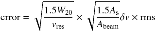 (4)where As is the surface area of the source and Abeam is the surface area of the synthesised beam. The integrated value of the pixel values is used, rather than the integral of the Gaussian fit, to be more sensitive to possible extended emission which is likely to be suppressed by the wings of the Gaussian.
2.7. Flux correction
 |
Fig. 7 Beam response of pointings in the mosaic as function of the observed declination (δ) (top panel) and the NCP projected declination (M). The observed mosaic is Nyquist sampled, with a regular interval between beams of 15 arcmin. When projecting the data, the sampling becomes different. |
We have noticed a shortcoming in the invert task within miriad when the data is converted from the u,v plane to the image plane. When creating the mosaiced image, each individual pointing is inverted and then the set of images are combined using the primary beam model for the relative weightings.
When gridding the data using the NCP projection the offset in declination with respect to the tangential point is calculated using Eq. (2). In this function δ0 is the central declination, δ is the observed declination that has to be gridded and Δα is the difference between the central Right Ascension and the Right Ascension to be gridded. At declinations close to zero, the differences in M in the projected frame become very small: δ = 0 + ϵ and δ = 0 + 2ϵ are gridded to the same pixel in the projected frame and for δ = 0 there is a singularity as there is no solution at all.
In the observed frame, the mosaic is Nyquist sampled and there is a pointing every 15 arcmin between 0.25 and 10 degrees in declinations. This is shown in the top panel of Fig. 7 where the response of each beam is plotted as function of declination. At each position the sum of all the beam responses is equal and the weighted sum is always unity.
The separation between the pointings with respect to each other changes, when they are converted to the projected NCP frame. Not only the position of pointings changes, the complete shape of the primary beam becomes different, and a distorted beam should be applied when doing the weighting. We suspect that this is not happening and that the undistorted beam is used. This is demonstrated in the bottom panel of Fig. 7 where the undistorted beam response of the pointings is plotted as function of the projected M value. The M value gives the offset with respect to the reference pixel, so M = 0 corresponds to δ = 5 degrees.
In an image the flux is determined by the weighted sum of the beam response of all the contributing pointings.: 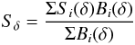 (5)and
 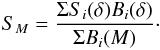 (6)Where Si(δ) is the measured flux by a pointing, Bi(δ) is the beam response in the observed frame, while Bi(M) is the beam response in the projected frame.
In the projected frame the sum of the beam responses changes dramatically with declination if the projection is not applied to the shape of the primary beam.
As a result, fluxes appear lower in the projected frame at low declinations, as the sum of the beam responses by which the flux is weighted is larger. At high declinations the opposite is the case where the flux values in the projected frame become enhanced.
This effect is clearly visible in the data, as the measured flux of objects at low declination is systematically to low. This is demonstrated for a sample of objects in the right panel of Fig. 8. The data points show the ratio between the fluxes obtained from the WVFS total power data as described in chapter 4 and the fluxes from the cross-correlation data, without a flux correction. The flux ratios are plotted on a logarithmic scale against declination. At low declinations the total power fluxes are much higher, while at high declinations the opposite is the case.
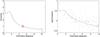 |
Fig. 8 Left panel: correction factor as function of declination, to be applied on the obtained fluxes. Right panel: correcting factor on a logarithmic scales with data points representing the flux ratio between WVFS total-power and cross-correlation data, before applying the correction on the cross-correlation data. |
The correction that has to be applied is given by: 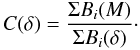 (7)This ratio is plotted in the left panel of Fig. 8 as function of declination. The cross indicates the central position of the projected grid at 5 degrees, where the ratio is exactly 1 as no correction has to be applied. For declinations below 5 degrees the fluxes have to be scaled up, while for high declinations the fluxes have to be scaled down. At both ends of the correction function there is a bump, as the edges of the mosaic are not Nyquist sampled in the observations, so the integrated beam responses are different here. For declinations approaching zero degrees the correction goes to infinity, because of the singularity in the NCP projection here.
In the right panel of Fig. 8 the same correcting ratio is plotted on a logarithmic scale, together with a sample of data points as described before. Although the scatter is large the data points follow the correcting function reasonably well. The fluxes obtained from the total power and cross-correlation data actually can be different as the total power data is more sensitive to extended emission, but to get the cross-correlation data on the right level, the correction has to be applied.
3. Results
3.1. Source detection
Because of the large extent of the WVFS, and the large number of independent pixels, an automated source finding algorithm is essential to obtain a list of candidate detections. Although the sensitivity of the data is good, source detection is not straightforward because of the artifacts that are apparent in the data as described in Sect. 2.5. Two strategies have been employed to circumvent these complications and to obtain a list of candidate detections that is as complete as possible. The first method is a blind search that uses a clipping level of 8σ. This conservative clipping level will provide a reliable list of bright features. The second method uses a less conservative clipping level of 5σ that will also yield many false positives. An extra constraint on these features is that an optical counterpart is required within a suitable search radius and at a comparable radial velocity. The search radius is variable, depending on the declination of the candidate feature, as will be explained below.
For both approaches the Duchamp (Whiting 2008) source finding algorithm has been used, with different control parameters. The two methods and their results are described below. When searching for objects, Duchamp uses the processed, three dimensional data cubes. The source finder has been run on each of the 18 cubes individually, although for Cubes 8 and 9 every pixel above a declination of 9 degrees has been blanked. This region could not be used due to solar interference, which heavily affected the quality of the data. The interference is so strong here that it increases the noise and causes many false and unreliable detections. As a consequence, any objects between ~172 and ~190 degrees in right ascension and above 9 degrees in declination will not be detected.
3.2. Blind detections
Although the noise in the data is approximately Gaussian, it is clear from an inspection of the histogram of brightnesses that there are excess negative outliers from this ideal distribution. Due to the purely relative nature of interferometric data (the absence of the auto-correlation), artifacts caused by e.g. side-lobes, continuum sources and solar interference are symmetric in their positive and negative excursions with respect to zero. For this reason, the number of noise and artifact pixels within a negative brightness interval is equal to the number of likely false positive pixels within the same brightness interval on the positive side of the histogram. This is illustrated in Fig. 9 where a histogram of the observed brightness is plotted from the central portion of Cube 13. The incidence of each brightness scaled by the local rms fluctuation level is plotted. At 4 or 5σ the number of negative pixels is still significant, but these rapidly drop to zero for a brightness below − 8σ. A clipping level of +8σ was therefore chosen since it should yield no false positive detections due to either noise or artifacts.
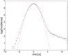 |
Fig. 9 Histogram of incidence of brightness in units of σ in Cube 13 of the WVFS. At a level of − 5σ there are still many pixels, indicating that the number of false positives at the + 5σ level is also likely to be relatively high. At a level of − 8σ there are no negative pixels, so above a clipping level of + 8σ no false detections are expected. |
For the actual source finding Duchamp has been used with four different settings, that are summarised in Table 2. The cubes were first Hanning smoothed to velocity resolutions of 16, 32, 64 and 128 km s-1, to be more sensitive to sources with different line widths. Although an initial clipping level of 8σ has been used for peak identification, the detected features are “grown” to a level of 3σ. Furthermore a certain number of pixels in the velocity domain is required, that is representative for the velocity resolution.
Duchamp parameters for the blind H i search in the WVFS cross-correlations.
 |
Fig. 10 Example of a source with a bright residual side-lobe pattern. An X pattern is clearly visible and those regions within the side-lobes with multiple contours might be mis-identified as individual objects by the Duchamp source-finding algorithm. |
For each candidate detection, the spectrum was determined and a moment map has been created by integrating the data cube over the velocity width of the detection. Furthermore, an optical counterpart was sought for each source within a radius of 7 arcmin. A radius of 7 arcmin was chosen both to accomodate some intrinsic offset of the H i and optical centroid as well as those instances of limited positional accuracy, as will be explained below.
All spectra and moment maps were inspected visually, to look for artifacts. Continuum artifacts, or solar interference can result in a false detection, but are easily recognised by eye.
The moment maps were used to eliminate those candidate sources coincident with residual side-lobe artifacts. When candidate sources are coincident with one of the arms of the X-shaped residual side-lobe of a bright nearby source, then they are very likely unreliable. An example of a clear residual side-lobe structure is shown in Fig. 10.
Furthermore, all multiple detections of the same source were excluded from the list of detections. Features that are at the edge of a cube are likely to be detected twice in two adjacent cubes. In the cubes with different velocity resolution, the peak flux of the candidate is not always at the same spatial position, resulting in a slightly different apparent centroid. Finally, sources are sometimes counted twice when there are two bright spectral components that do not connect. For example in the case of a double horned profile, where the region between the two peaks does not exceed the 3σ level which was set as the “growing” limit.
Physical properties of new H i detections in the Westerbork Virgo Filament Survey.
A total of 135 sources have been detected using the blind detection approach, which have a peak brightness exceeding 8σ. The properties of each detection are listed in the Appendix, where the spectrum of each detection is shown as well. The first column gives the name of the source, consisting of the characters “WVFSCC” (Westerbork Virgo Filament Survey Cross-Correlation), followed by six plus six digits for the Right Ascension and Declination respectively in hh:mm:ss and dd:mm:ss format. The second column gives the optical ID if present, followed by the Right Ascension, Declination and Velocity. The sixth and seventh column give the line-width at 50 and 20% of the peak (W50 and W20). The following three columns give the integrated line-strength (Sl), the integrated moment map flux density (Si) and the error in the integrated flux density (σS). The differences between the different flux measurements and the method of estimating the uncertainty are explained in Sect. 3.4. The last column in the table indicates whether the object has been found in the blind search (B) or in the search where an optical identification is required (O). When objects appear in both search methods, this is indicated with two letters.
Of the 135 detected sources in the blind search method, only WVFSCC 120929+080730 does not have an optical counterpart, the properties of this objects are given in Table 3, which has the same column description as the Appendix, but only showing new H i detections in the survey.
3.3. Confirmed detections
Because of the high clipping limit in the blind search, many objects have been missed that are at a lower significance, which might still be real sources. In a second approach, all features are sought with a peak brightness of at least 5σ. This limit was chosen to permit the deepest possible search for the H i counterparts to known objects while keeping the number of likely false positives manageable. An optical identification was sought for each candidate within a variable search radius, using the NASA Extragalactic Database (NED)1. Only those features which have an optical counterpart at a radial velocity that is within 100 km s-1 of the detected feature are accepted. Because the survey has been done using an east-west array, the synthesized beam size is increasing towards lower declinations. For features above 8 degrees in declination, a search radius of 6 arcmin was employed, which is on the order of the synthesized beam FWHM. For lower declinations, the search radius is scaled as a function of the declination:  (8)For declinations below 2 degrees a constant search radius of 24 arcmin is used, which is of the same order as the primary beam of the telescope. This scaling is chosen to track the distortions of the NCP projection at these low declinations. Allowing even larger search radii is not necessary, as the uncertainty in position cannot be larger than the primary beam.
A very similar method has been used to identify counterpart features as for the blind search, employing Duchamp with two different settings, as given in Table 4. Only two velocity resolutions have been used, as using more combinations did not appear to be practical. The list of candidate features was visually inspected in a very similar way as the blind search detections. Multiple detections were omitted, as well as false positives caused by artifacts in the data.
Duchamp parameters for the counterpart search in the WVFS.
In a similar fashion as for the blind search, all the spectra and moment maps of the candidate features have been inspected visually to look for artifacts. All detections with their properties are listed in the appendix, together with the sources that have been detected through the blind detection.
A total of 198 H i features with a peak brightness exceeding 5σ could be identified with an optical counterpart within the search radius. We have compared the list of detections with the HIPASS catalogue. In total 53 objects are not listed in the HIPASS database, of which 16 are completely new H i detections. On the other hand 51 objects have not been detected in the current data, which are listed in the HIPASS catalogue. The properties of the new H i detections are listed in Table 3.
The WVFS has a better point source sensitivity than HIPASS, which explains the sources that are detected in WVFS and not in HIPASS. For the HIPASS detections, a clipping level of 4σ has been used which corresponds to approximately 60 mJy beam-1 over 18 km s-1 taking into account the point source sensitivity of the original HIPASS cubes. The 5σ clipping limit that has been used in this survey corresponds to ~30 mJy beam-1 at a very comparable velocity resolution of 16 km s-1.
Although the point source sensitivity of the WVFS is almost a factor two better than HIPASS, the latter has a much better brightness sensitivity due to the larger beam. The 14 arcmin beam of the Parkes telescope is approximately six times larger in area than the synthesised beam of the WVFS, resulting in a three times better brightness sensitivity. This may explain the relatively high number of sources that have not been detected in the WVFS. Diffuse sources will be more easily detected in the larger beam of a single dish like the Parkes telescope.
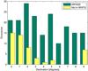 |
Fig. 11 The dark histogram shows the number of HIPASS sources as function of declination between 0 and 10 degrees, binned in intervals of 1 degree. The light histogram shows the number of HIPASS objects that have not been found in the WVFS source detection procedures. The distribution of undetected sources is not uniform, as their proportion increases toward lower Declination. |
The incidence of all the 51 HIPASS sources that are missed in the current survey are plotted as a histogram of declination with a bin size of 1 degree in Fig. 11. The dark bars of the histogram represent the distribution of sources catalogued by HIPASS, while the light coloured bars show the number of HIPASS sources that have not been detected by WVFS. The histogram does not show a uniform distribution for the missed sources, several sources that have not been identified in WVFS are in the region that has been excluded from the search due to solar interferences, as explained in Sect. 3.1. This explains the high number of non-detections in the last bin, above a declination of 9 degrees. What is striking is that the vast majority of the sources that have not been detected in the WVFS cross-correlation data have a low Declination. This is again an effect of the shortcoming in the gridding, as has been described earlier. At declinations below 2 degrees the projected fluxes become diluted by a factor more than two and in many cases end up below the detection limit.
3.4. Flux comparison
The two different methods by which the flux was determined are compared in Fig. 12 where the integrated flux is plotted as function of the line-strength. The dashed line through the origin of the plot indicates where the fluxes are equal. For low flux values, there is reasonable agreement between the two methods. For high fluxes the differences are increasing dramatically, with most bright sources being much more extended than the synthesised beam. This is shown in a different way in Fig. 13, where the ratio of the two fluxes with their error bars is plotted on a logarithmic scale against the integrated flux on a logarithmic scale. Here the differences become even more apparent. In addition to a systematically higher flux in all the integrated moment maps, the ratio also increases with source brightness. This result implies that most objects do have extended emission on the scale of the ~5 arcmin synthesised beam.
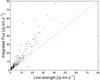 |
Fig. 12 Integrated flux of the WVFS cross correlation data plotted against the line-strength. For many objects, the integrated flux is significantly larger than the line strength implying that detections are spatially resolved. |
As a second test, all measured fluxes have been compared with fluxes obtained from the HIPASS catalogue, where available. Figure 14 shows both the WVFS line-strength (circles) as the integrated flux (crosses) plotted against HIPASS fluxes. The dashed line indicates where the plotted fluxes are equal. Fluxes determined from the line-strength measurement are much too low; while there is reasonable correspondence between the integrated WVFS fluxes and the HIPASS fluxes. This is also shown in Fig. 15, where the ratio between the integrated WVFS fluxes and the HIPASS fluxes is plotted on a logarithmic scale against the HIPASS fluxes. At low flux values the scatter is very large, but overall there is very good correspondence. To be less influenced by the scatter, for all objects with a HIPASS flux stronger than 5 Jy km s-1 the mean and median values have been determined. The mean of the ratios is 0.91 with a standard deviation of 0.33, while the median of the ratios is 0.87, these numbers indicate that there is an excess in the catalogued HIPASS fluxes of ~10% with respect to the WVFS cross-correlation data.
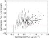 |
Fig. 13 Ratio of integrated flux and line-strength is plotted on a logarithmic scale as function of the integrated flux. For almost all sources the emission is more extended than the synthesised beam and the integrated flux is much higher than the integrated line-strength. |
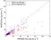 |
Fig. 14 WVFS line-strength (circles) and integrated flux (crosses) are plotted as function of HIPASS flux. Although the line-strength is very low for many objects with respect to the HIPASS fluxes, there is good correspondence between the HIPASS data and the WVFS integrated fluxes. |
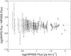 |
Fig. 15 Ratio of WVFS integrated flux and HIPASS fluxes as function of HIPASS fluxes, plotted on a logarithmic scale. |
3.5. New H I detections
Both the blind search for neutral hydrogen and the search based on identification of an optical counterpart have resulted in a number of new H i detections. Spectra for all these detections are shown in Fig. 16; WVFSCC 120929+080730 is the only one without an optical counterpart. Typically all detections have a peak brightness of between 25 and 50 mJy beam-1, which is quite faint. Based on the fluxes derived from WVFS, none of these sources could have been detected by HIPASS, as the peak flux is below the clipping level that has been utilised for the HIPASS source finding. The new H i detections do not share any particular attributes, and the spectra have a variety of shapes. The line-widths vary from a few tens of km s-1 to several hundreds of km s-1 and both single peaks as well as “double-horned” profiles are encountered.
3.6. H I without an optical counterpart
The blind H i search resulted in one source, for which no optical counterpart is found. WVFSCC 120929+080730 is just at the 8σ detection limit of the blind H i search. This feature has one strong peak, but has a relatively narrow line-width of only 22 km s-1 at FWHM as can be seen from the spectrum in Fig. 16. The peak column density of this feature is NHI ~ 1.5 × 10¹⁹ km s-1. No cataloged optical counterpart is found within a radius of one degree, at the relevant velocity. The nature of this detection is not clear, as the DSS image of this position also shows no likely counterpart. Possibly this is an example of an intergalactic gas filament that is a component of the Cosmic Web. Comparison with other data products will have to reveal whether this detection can be confirmed in independent data.
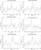 |
Fig. 16 Spectra of new H i detections is the WVFS cross correlation data. The central velocity of each object is indicated by the dashed vertical line. |
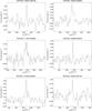 |
Fig. 16 continued. |
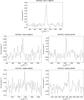 |
Fig. 16 continued. |
3.7. Extended neutral hydrogen
For each detection a moment map has been created by integrating the cubes in the velocity domain over the line-width of the detection. All integrated maps were visually inspected to search for extended emission or companions. For several galaxies there is clear evidence of extended H i emission; we will discuss these cases in more detail individually.
WVFSCC 103109+042831: the main galaxy UGC 5708 has a clear extension toward a nearby companion to the north west. The companion is separated from UGC 5708 by approximately 20 arcmin, which corresponds to 100 kpc. Both the radial velocity and the line width of the companion are very similar to that of UGC 5708 as can be seen from the spectra in Fig. 17. The peak column density of the companion is NHI ~ 3 × 1019 cm-2. The contours are overlaid on a second generation DSS image. An optical counterpart can be identified exactly at the peak of the contours. This optical counterpart is probably CGCG 037-059 which is classified as a galaxy triplet. Only one radial velocity, of 11 944 km s-1 is known for this triplet. If CGCG 037-059 is indeed a galaxy triplet that is gravitationally bound, then a relation with the H i gas is not likely because of the very large deviation in radial velocity and the similarity in spatial position is purely coincidental. The other possibility is that the classification of CGCG 037-059 is incorrect and that the H i gas is associated with an object with an unknown redshift.
WVFSCC 123428+062753: the main galaxy is NGC 4532, that has an extended H i companion towards the south east as can be seen in Fig. 18. Although the gas looks very extended, it belongs to the irregular galaxy Holmberg VII, at a radial velocity of 2039 km s-1. Due to the relatively large synthesised beam it has not been identified as an individual object, but this is not the first detection of neutral hydrogen in this galaxy.
WVFSCC 125550+041348: this is a very extended structure with at least 4 concentraions as can be seen in Fig. 19. The main galaxy is NGC 4808, which has a long tail of H i gas towards the south. The apparent extension to the south-east is most likely caused by a residual side-lobe. When looking at the optical DSS image with the H i contours overlaid, an optical counterpart can be identified for all H i peaks. The first optical galaxy south-east of NGC 4808 is CGCG 043-077 and has only one H i contour. The peak column density of this detection is NHI ~ 1.4 × 1019 cm-2, this is the first H i detection of this galaxy. The two galaxies to the south are UGC 8053 and UGC 8055, both with a peak column density of NHI ~ 4 × 1019 cm-2, which have been previously detected in H i .
4. Discussion and conclusion
The WSRT has been used in a very novel observing mode to simulate a filled aperture in projection of 300 × 25 m by observing at very extreme hour angles. Because of the very short observing times per pointing it is a technical challenge to observe and reduce this data, while still achieving useful results. In total 22 000 pointings have been observed that cover a total area of ~1500 square degrees. Each pointing has been observed two times for a period of one minute. Normally an integration time of one minute with an interferometer is not sufficient to fill the u,v plane, however as there are essentially no gaps between the individual antennas in projection, and the two scans have a complimentary orientation, a well defined synthesized beam could be formed. The observing method is limited to a narrow range in declination, but has been very successful.
In the reduced data we reach a flux sensitivity of ~6 mJy beam-1 over 16 km s-1. The synthesised beam has an average size of 395 × 245 arcsec, which results in a brightness sensitivity of NHI ~ 1018 cm-2. Such a brightness sensitivity can typically only be achieved with single-dish observations. Because the WSRT is an interferometer, the calibration and stability of the bandpass is significantly superior to that of a single dish.
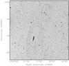 |
Fig. 17 A second generation red band DSS image, overlaid with H i contours of WVFSCC 103109+042831. Contour levels are drawn at 1, 2, 4 and 8 Jy km s-1. The main galaxy is UGC 5708, the small companion in the north west is most likely CGCG 037-059 |
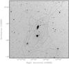 |
Fig. 18 H i contours of WVFSCC 123428+062753 at 1, 2, 4 and 8 Jy km s-1 are overlaid on a second generation DSS images. The main galaxy is NGC 4532, while the diffuse galaxy in the South-East that is attached is Holmberg VII. |
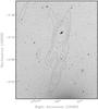 |
Fig. 19 H i contours of WVFSCC 125550+041348 at levels of 1, 2, 4 and 8 Jy km s-1 overlaid on a red band, second generation DSS images. The main galaxy NGC 4808 has a long tail of H i towards the south, connecting two other galaxies. South-East of the main galaxy is a very faint signal possibly associated with another galaxy. |
The drawback of interferometric observations is that a cleaning step has to be applied to correct for the synthesised beam shape, especially for bright objects. Although the synthesised beam is well defined, the side-lobes in our observations are very strong, making the cleaning step a critical one. Because of the large size of the survey, only one pass of cleaning deconvolution could be applied. Improved deconvolution results would require detailed masking of real emission features during component identification. Because of the relatively high side-lobe level, any automatic masking procedure is unlikely to be reliable. Each emission peak would have to be inspected visually, to be able to distinguish a real emission feature from a side-lobe artifact. Because of the size of the survey this approach was not considered practical. As a result of these limitations, there are low level artifacts in the data, although the flux sensitivity in the reduced data is very good.
An extra complication in processing the data is that the north-south synthesized beamsize increases towards low Declinations since the WSRT is an east-west array. Furthermore, the natural image plane projection of an east-west array is the North Celestial Pole (NCP) projection (Brouw 1971) which becomes undefined at zero degrees. As a result, only positive declinations could be analysed in our mosaiced images. Although this did not dramatically affect our results, it is still a major point of concern.
We found another serious complication in using an NCP projection in a wide field survey close to a declination of zero degrees. This complication is not caused by a shortcoming in the projection, but more likely a shortcoming in the imaging software that has been used. When gridding the observed data or u,v coordinates to the projected plane, the observed flux is not being conserved due to an incorrect wighting when combining pointings in a mosaic. At positive declinations, the imaged flux of data below the declination of the reference pixel is diluted while for data above the reference pixel the imaged flux is enhanced compared to the observed flux. This effect is very apparent when using a NCP projection but probably also happens when using other projections. When observing small fields, or fields between ~20 and ~70 degrees in declination this effect is negligible, however in our case a significant correction to the derived fluxes had to be applied.
In general, other image plane projections are required at Declinations near zero degrees to enable both positive and negative Declinations to be imaged simultaneously. However several major interferometers are East-West arrays, including the WSRT and the Australia Telescope Compact Array (ATCA). All these telescopes are being upgraded, partly to serve as a pathfinders for the SKA (Square Kilometre Array). A general aim of future telescopes, especially the ones that use a FPA (Focal Plane Array) is to conduct large surveys of the entire sky. Ideally these surveys will have significant overlap with deep optical surveys, however several major optical surveys are concentrated at Declinations near zero degrees.
Two search methods have been applied to the reduced WVFS data, both using the Duchamp source finding algorithm. The first method is a blind search at a peak brightness limit of 8σ. The second method uses an initial peak brightness limit of 5σ, but has the additional requirement that all detected features need to have an optical counterpart. In the blind search 138 objects have been detected, while the second search resulted in 198 H i counterparts to cataloged optical galaxies. Of all the detections 16 are new H i detections and only 1 detection does not have an optical counterpart. On average, the interferometric total fluxes of detections are ~10% lower than the catalogued fluxes in the HIPASS archive.
There are many features in the cube with a peak of 3 or 4σ and an integrated flux that probably exceeds 8σ. It is very likely that many of these features are real, however they cannot be identified reliably by automated source finders. In a subsequent paper, the WVFS cross-correlation data will be compared with the WVFS total-power data and the re-reduced HIPASS data as described in Popping & Braun (2011a) and Popping & Braun (2011b). Both surveys contain several new H i detections and tentative filaments. As this is a limited number of sources, we can do a targeted search in the WVFS cross-correlation data. Although the brightness sensitivity of each of the three surveys is almost an order of magnitude different, comparison of the data will be useful to distinguish extended and diffuse emission from denser H i clumps.
Online material
Appendix A: Physical properties of H i detections in the Westerbork Virgo Filament Survey
Physical properties of H i detections in the Westerbork Virgo Filament Survey.
Appendix B: Spectra of all H i detections in the WVFS cross-correlation data
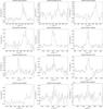 |
Fig. B.1 Spectra of detections of neutral hydrogen in the WVFS cross-correlation with a known optical counterpart. Detections were found using an 5σ threshold and are only accepted if an optical counterpart at a corresponding redshift is cataloged. The central velocity of each object is indicated by the dashed line. |
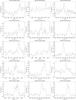 |
Fig. B.1 continued. |
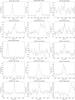 |
Fig. B.1 continued. |
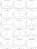 |
Fig. B.1 continued. |
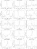 |
Fig. B.1 continued. |
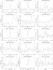 |
Fig. B.1 continued. |
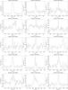 |
Fig. B.1 continued. |
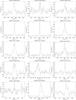 |
Fig. B.1 continued. |
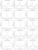 |
Fig. B.1 continued. |
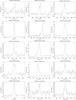 |
Fig. B.1 continued. |
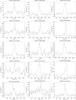 |
Fig. B.1 continued. |
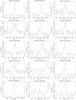 |
Fig. B.1 continued. |
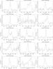 |
Fig. B.1 continued. |
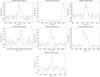 |
Fig. B.1 continued. |
The NASA/IPAC Extragalactic Database (NED) is operated by the Jet Propulsion Laboratory, California Institute of Technology, under contract with the National Aeronautics and Space Administration.
Acknowledgments
The Westerbork Synthesis Radio Telescope is oper- ated by the ASTRON (Netherlands Foundation for Research in Astronomy) with support from the Netherlands Foundation for Scientic Research (NWO).
References
- Barnes, D. G., Staveley-Smith, L., de Blok, W. J. G., et al. 2001, MNRAS, 322, 486 [NASA ADS] [CrossRef] [Google Scholar]
- Brouw, W. N. 1971, PhD Thesis, Leiden University [Google Scholar]
- Cen, R., & Ostriker, J. P. 1999, ApJ, 514, 1 [NASA ADS] [CrossRef] [Google Scholar]
- Davé, R., Hernquist, L., Katz, N., & Weinberg, D. H. 1999, ApJ, 511, 521 [NASA ADS] [CrossRef] [Google Scholar]
- Fomalont, E. 1981, Newsletter. NRAO NO. 3, 3 [Google Scholar]
- Lehner, N., Savage, B. D., Richter, P., et al. 2007, ApJ, 658, 680 [NASA ADS] [CrossRef] [Google Scholar]
- Popping, A. 2010, PhD Thesis (University of Groningen) [Google Scholar]
- Popping, A., & Braun, R. 2011a, A&A, 527, A90 [NASA ADS] [EDP Sciences] [Google Scholar]
- Popping, A., & Braun, R. 2011b, A&A, submitted [Google Scholar]
- Sault, R. J., Teuben, P. J., & Wright, M. C. H. 1995, in Astronomical Data Analysis Software and Systems IV, ASP Conf. Ser. 77, 433 [Google Scholar]
- Tripp, T. M., Sembach, K. R., Bowen, D. V., et al. 2008, ApJS, 177, 39 [NASA ADS] [CrossRef] [Google Scholar]
- Whiting, M. T. 2008, Astronomers! Do You Know Where Your Galaxies are? ed. H. Jerjen, & B. S. Koribalski, 343 [Google Scholar]
- Wong, O. I., Ryan-Weber, E. V., Garcia-Appadoo, D. A., et al. 2006, MNRAS, 371, 1855 [NASA ADS] [CrossRef] [Google Scholar]
All Tables
Right ascension range and noise levels of the 18 individual sub-cubes of the WVFS cross-correlation data.
Physical properties of new H i detections in the Westerbork Virgo Filament Survey.
All Figures
|
Fig. 1 Observing mode of the WSRT dishes: 12 of the 14 dishes are placed at a regular interval of 144 meters. When observing at large hour angles, an approximately filled aperture of 300 by 25 m can be simulated in projection. |
| In the text | |
|
Fig. 2 Due to the filled aperture of ~300 × 25 meters, a very elongated beam is created. By observing each pointing twice at complementary orientations, the combined beam of the two observations is nearly circular, although with a significant side-lobe level. |
| In the text | |
|
Fig. 3 Example of a channel map from one of the processed sub-region cubes (Cube 9) from the WVFS cross-correlation data. The inner region is well sampled by the pointings and the noise is uniform, while emission at the edges is noisier. There is 25% overlap in right ascension between adjacent cubes. Unfortunately the coordinates could not be shown in this plot due to projection effects, as explained in the text. |
| In the text | |
|
Fig. 4 Same image as Fig. 3, but now with the positions of the pointings overlaid. Each cube contains data from 45 pointings in declination, by 40 pointings in right ascension covering 11 by 10 degrees. Due to the NCP projection of the data, the declinations close to zero degrees are increasingly distorted, as can be seen in the shape of the pointings that are squeezed toward the lowest declinations. Unfortunately, pointings with both positive and negative declinations could not gridded simultaneously due to limitations of the NCP projection. |
| In the text | |
|
Fig. 5 Beam shape of a central pointing in the strip at Dec = 10 degrees. The left panel shows the synthesized beam of a single observation, while the right panel shows the beam for the combination of two complimentary scans. Both panels have the same intensity scale and contours are drawn at 70, 80 and 90 percent of the peak. |
| In the text | |
|
Fig. 6 The left panel shows a region of the dirty map; data that has only been inverted from the u,v plane to the image plane. The right panel shows exactly the same region after one pass of cleaning. While in the left panel the cross pattern of the beam is very apparent, in the right panel the side-lobes are almost completely subtracted. |
| In the text | |
|
Fig. 7 Beam response of pointings in the mosaic as function of the observed declination (δ) (top panel) and the NCP projected declination (M). The observed mosaic is Nyquist sampled, with a regular interval between beams of 15 arcmin. When projecting the data, the sampling becomes different. |
| In the text | |
|
Fig. 8 Left panel: correction factor as function of declination, to be applied on the obtained fluxes. Right panel: correcting factor on a logarithmic scales with data points representing the flux ratio between WVFS total-power and cross-correlation data, before applying the correction on the cross-correlation data. |
| In the text | |
|
Fig. 9 Histogram of incidence of brightness in units of σ in Cube 13 of the WVFS. At a level of − 5σ there are still many pixels, indicating that the number of false positives at the + 5σ level is also likely to be relatively high. At a level of − 8σ there are no negative pixels, so above a clipping level of + 8σ no false detections are expected. |
| In the text | |
|
Fig. 10 Example of a source with a bright residual side-lobe pattern. An X pattern is clearly visible and those regions within the side-lobes with multiple contours might be mis-identified as individual objects by the Duchamp source-finding algorithm. |
| In the text | |
|
Fig. 11 The dark histogram shows the number of HIPASS sources as function of declination between 0 and 10 degrees, binned in intervals of 1 degree. The light histogram shows the number of HIPASS objects that have not been found in the WVFS source detection procedures. The distribution of undetected sources is not uniform, as their proportion increases toward lower Declination. |
| In the text | |
|
Fig. 12 Integrated flux of the WVFS cross correlation data plotted against the line-strength. For many objects, the integrated flux is significantly larger than the line strength implying that detections are spatially resolved. |
| In the text | |
|
Fig. 13 Ratio of integrated flux and line-strength is plotted on a logarithmic scale as function of the integrated flux. For almost all sources the emission is more extended than the synthesised beam and the integrated flux is much higher than the integrated line-strength. |
| In the text | |
|
Fig. 14 WVFS line-strength (circles) and integrated flux (crosses) are plotted as function of HIPASS flux. Although the line-strength is very low for many objects with respect to the HIPASS fluxes, there is good correspondence between the HIPASS data and the WVFS integrated fluxes. |
| In the text | |
|
Fig. 15 Ratio of WVFS integrated flux and HIPASS fluxes as function of HIPASS fluxes, plotted on a logarithmic scale. |
| In the text | |
|
Fig. 16 Spectra of new H i detections is the WVFS cross correlation data. The central velocity of each object is indicated by the dashed vertical line. |
| In the text | |
|
Fig. 16 continued. |
| In the text | |
|
Fig. 16 continued. |
| In the text | |
|
Fig. 17 A second generation red band DSS image, overlaid with H i contours of WVFSCC 103109+042831. Contour levels are drawn at 1, 2, 4 and 8 Jy km s-1. The main galaxy is UGC 5708, the small companion in the north west is most likely CGCG 037-059 |
| In the text | |
|
Fig. 18 H i contours of WVFSCC 123428+062753 at 1, 2, 4 and 8 Jy km s-1 are overlaid on a second generation DSS images. The main galaxy is NGC 4532, while the diffuse galaxy in the South-East that is attached is Holmberg VII. |
| In the text | |
|
Fig. 19 H i contours of WVFSCC 125550+041348 at levels of 1, 2, 4 and 8 Jy km s-1 overlaid on a red band, second generation DSS images. The main galaxy NGC 4808 has a long tail of H i towards the south, connecting two other galaxies. South-East of the main galaxy is a very faint signal possibly associated with another galaxy. |
| In the text | |
|
Fig. B.1 Spectra of detections of neutral hydrogen in the WVFS cross-correlation with a known optical counterpart. Detections were found using an 5σ threshold and are only accepted if an optical counterpart at a corresponding redshift is cataloged. The central velocity of each object is indicated by the dashed line. |
| In the text | |
|
Fig. B.1 continued. |
| In the text | |
|
Fig. B.1 continued. |
| In the text | |
|
Fig. B.1 continued. |
| In the text | |
|
Fig. B.1 continued. |
| In the text | |
|
Fig. B.1 continued. |
| In the text | |
|
Fig. B.1 continued. |
| In the text | |
|
Fig. B.1 continued. |
| In the text | |
|
Fig. B.1 continued. |
| In the text | |
|
Fig. B.1 continued. |
| In the text | |
|
Fig. B.1 continued. |
| In the text | |
|
Fig. B.1 continued. |
| In the text | |
|
Fig. B.1 continued. |
| In the text | |
|
Fig. B.1 continued. |
| In the text | |
Current usage metrics show cumulative count of Article Views (full-text article views including HTML views, PDF and ePub downloads, according to the available data) and Abstracts Views on Vision4Press platform.
Data correspond to usage on the plateform after 2015. The current usage metrics is available 48-96 hours after online publication and is updated daily on week days.
Initial download of the metrics may take a while.