| Issue |
A&A
Volume 528, April 2011
|
|
|---|---|---|
| Article Number | A92 | |
| Number of page(s) | 17 | |
| Section | Galactic structure, stellar clusters and populations | |
| DOI | https://doi.org/10.1051/0004-6361/201015226 | |
| Published online | 07 March 2011 | |
The Hamburg/ESO R-process Enhanced Star survey (HERES)
VI. The Galactic chemical evolution of silicon⋆,⋆⋆
1 Key Laboratory of Optical Astronomy, National Astronomical Observatories, CAS, 20A Datun Road, Chaoyang District, 100012 Beijing, PR China
e-mail: This email address is being protected from spambots. You need JavaScript enabled to view it.
2 Graduate University of the Chinese Academy of Sciences, 19A Yuquan Road, Shijingshan District, 100049 Beijing, PR China
3 Sydney Institute for Astronomy (SIfA), School of Physics, The University of Sydney, NSW 2006, Australia
4 Zentrum für Astronomie der Universität Heidelberg, Landessternwarte, Königstuhl 12, 69117 Heidelberg, Germany
5 Division of Astronomy and Space Physics, Department of Physics and Astronomy, Uppsala University, Box 516, 75120 Uppsala, Sweden
Received: 17 June 2010
Accepted: 20 January 2011
Abstract
Aims. To obtain detailed silicon abundances of metal-poor stars, we aim to explore the correlation between the abundance ratios and the stellar parameters and the chemical enrichment of the interstellar medium (ISM).
Methods. We determined the silicon abundances of 253 metal-poor stars in the metallicity range −4 < [Fe/H] < −1.5, based on non-local thermodynamic equilibrium (NLTE) line formation calculations of neutral silicon and high-resolution spectra obtained with VLT-UT2/UVES.
Results. The Teff dependence of [Si/Fe] noticed in previous investigations is diminished in our abundance analysis owing to the inclusion of NLTE effects. An increasing slope of [Si/Fe] towards decreasing metallicity is present in our results, in agreement with Galactic chemical evolution models. Intrinsic scatter of [Si/Fe] in our sample is small. We identified two dwarfs with [Si/Fe] ~ +1.0: HE 0131−3953, and HE 1430−1123. These main-sequence turnoff stars are also carbon-enhanced. They may have been pre-enriched by sub-luminous supernovae.
Conclusions. The small intrinsic scatter of [Si/Fe] in our sample may imply that these stars formed in a region where the yields of type II supernovae were mixed into a large volume, or that the formation of these stars was strongly clustered, even if the ISM was enriched by single SNa II in a small mixing volume.
Key words: line: formation / line: profiles / stars: abundances / stars: Population III / Galaxy: abundances / Galaxy: halo
Based on observations collected at the European Southern Observatory, Paranal, Chile (Proposal numbers 170.D-0010, and 280.D-5011).
Table 3 is only available in electronic form at http://www.aanda.org
© ESO, 2011
1. Introduction
Studying the detailed elemental abundances of metal-deficient stars in the Galactic halo is a standard approach to probe the origin of our Galaxy and its early evolution, because many of these stars have formed from the local counterparts to high-redshift gas clouds during the early chemo-dynamical evolution of the Galaxy (e.g. Beers & Christlieb 2005, and reference therein). While abundance ratios as a function of [Fe/H]1 provide information about the chemical enrichment history of the Galaxy, the scatter of these ratios allows us to study mixing processes of the interstellar medium (ISM) in the early phases of the formation of the Galaxy (e.g. Argast et al. 2000; Karlsson & Gustafsson 2005; Karlsson 2005).
In investigations of the enrichment of the ISM, the α-elements (e.g., Mg, Si, Ca, and Ti) are often used as tracer elements, because their yields depend on the mass and the explosion energy of the SN and the amount of fallback (Karlsson 2005). Silicon, which is produced by explosive oxygen burning, belongs to the most abundant metals, and it can be detected over a wide metallicity range. Besides, some extreme examples are found, which challenge the enrichment model of SNe II. For instance, HE 1424 − 0241, an extreme metal-poor star with [Fe/H] = −4.0, has a very low Si abundance (i.e., [Si/Fe] ~ −1.0 dex, Cohen et al. 2007). Therefore, Si is a suitable element to probe the enrichment of the ISM.
Previous studies of silicon abundances in metal-poor stars yielded a range of scatter in [Si/Fe]; typically from ~0.06 dex to 0.4 dex (e.g. Ryan et al. 1996; Cayrel et al. 2004; Cohen et al. 2004; Honda et al. 2004; Aoki et al. 2005; Preston et al. 2006; Lai et al. 2008; Shi et al. 2009). However, these dispersions cannot be simply considered as cosmic scatter reflecting the ISM mixing process. This is mainly because of three reasons: (1) the small sample size of analysis stars in most of the above-mentioned studies; (2) when several analyses from the literature are combined, systematic offsets in the Si abundances owing to different methods of stellar parameter determination and different structure of model atmospheres may arise, which artificially increases the scatter in the combined sample; (3) the Si abundance derived from the Si i line at 3905 Å, which is the only line that can be reliably measured in stars at [Fe/H] < −2.5 may not represent the true value, because this line may be contaminated by CH lines (Cayrel et al. 2004) and the abundance determined from this line shows an abnormal dependence on effective temperature (Teff) (Preston et al. 2006; Lai et al. 2008). All these may conceal the “real” cosmic scatter. Thus, Si abundances that are determined in a careful and homogeneous way for a large sample of metal-poor stars are needed.
Very recently, an NLTE analysis of silicon abundances of metal-poor stars has been carried out by Shi et al. (2009), who discuss the NLTE effects of the strong Si i lines at 3905 Å and 4103 Å. A strong correlation between the difference of [Si/Fe] calculated under NLTE and LTE assumptions of these two lines and the stellar parameters in their sample was noticed. This confirms the suggestion of Preston et al. (2006) that Si abundances determined from the Si i line at 3905 Å without NLTE corrections for metal-deficient star may not be considered as the true values at Teff warmer than 5800 K. From these results, the anomalous Teff dependence of [Si/Fe] (Preston et al. 2006; Lai et al. 2008) can be partially explained. Hence NLTE has to be taken into account when studying the chemical evolution of Si and the scatter of [Si/Fe] as a function of [Fe/H].
The aim of this work is thus to obtain detailed silicon abundances of metal-poor stars, and to explore the correlation between the abundance ratios and the stellar parameters and the chemical enrichment of the ISM are explored. This work is based on spectra of the Hamburg/ESO R-process Enhanced Star survey (HERES), as described in Sect. 2. The method and the procedures of the abundance analysis are described in Sect. 3. The results are presented in Sect. 4 and are discussed in Sect. 5.
2. Observations and stellar parameters
The present work is based on the spectra of 253 HERES stars. The sample selection and observations are described in Christlieb et al. (2004). For the convenience of the reader, we repeat here that the spectra were obtained with the Ultraviolet-Visual Échelle Spectrograph (UVES, Dekker et al. 2000) mounted on the 8 m Unit Telescope 2 (Kueyen) of the Very Large Telescope (VLT). The pipeline-reduced spectra cover the wavelength range from 3769 Å to 4980 Å at a minimum seeing-limited resolving power of R = 20 000. The coordinates and barycentric radial velocities of the stars are listed in Table 1 of Barklem et al. (2005, heareafter B05).
We adopt the stellar parameters of B05 in our analysis. In the work of B05, photometric Teff, metallicity estimated from the calibration of the Ca ii K-line index along with B − V color (Beers et al. 1999), log g estimated from log g − Teff correlation (Honda et al. 2004), ξ = 1.8 km s-1, and vmacro = 1.5 km s-1 were set as initial guess, and then were refined in an automated analysis that is based on the Spectroscopy Made Easy (SME) package by Valenti & Piskunov (1996). The details are described in Sects. 2 and 3 of B05.
3. Abundance analysis
In our analysis, we employ the one-dimensional line-blanked local thermodynamic equilibrium (LTE) model atmospheres MAFAGS (Fuhrmann et al. 1997), with opacity distribution functions (ODF) of Kurucz (1992). For consistency, solar abundances are the same as B05, i.e., C is taken from Allende Prieto et al. (2002) and other elements are those of Grevesse & Sauval (1998). During the computation of model atmospheres at [Fe/H] < − 0.6, an α-element enhancement of 0.4 dex is adopted. A convective efficiency of αmlt = 0.5 is used. For more details on the model atmospheres, we refer the reader to Grupp (2004).
3.1. Line synthesis
The silicon abundances were determined by spectrum synthesis of the Si i lines at 3905.53 Å and 4102.93 Å, using the Spectrum Investigation Utility (SIU) of Reetz (1991), which computes line formation under both LTE and NLTE conditions. Continuum scattering is considered in the computation of the source function.
Shi et al. (2009) studied the silicon abundance discrepancy between NLTE and LTE analyses for the two lines adopted in our analysis, and suggested that this departure is correlated with the strength of lines and stellar parameters. The main characteristics are: the NLTE effects of weak lines is small; the NLTE corrections of these two lines increase for extremely metal-poor warm stars, and the values can reach more than 0.15 dex for the 3905 Å line and 0.25 dex for the 4103 Å line. Thus, the NLTE effects of these two lines are considered in the present analysis. The silicon model atom and the NLTE calculation method are described in detail in Shi et al. (2008, 2009).
Atomic data of the Si i lines used in our analysis.
Molecular line data for B-X system of the CH molecule near 3905 Å from Kurucz (1993).
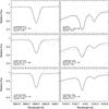 |
Fig. 1 Examples of spectral synthesis for six representative stars. The dots are the observational spectra, the solid lines are the best-fitting profile, and the dotted lines are the synthetic spectra with Si abundances of ± 0.15 dex with regard to the best fit, corresponding to less/more than 5% in the continuum. The listed parameters are Teff, log g, [Fe/H], and ξt, respectively. |
Another factor which may affect the determination of the silicon abundance is contamination with CH lines. Cohen et al. (2004) suggested that the Si i line at 3905.53 Å is probably blended with the B-X bandhead, which is located approximately at λ = 3900 Å. Preston et al. (2006) noticed that the blend effect of this CH band is weak in their sample of red horizontal-branch stars. However, the [C/Fe] ratio of most of their sample stars is less than 0.0 dex. Therefore, the CH B-X lines are included in our line synthesis to extract reasonable results for our metal-deficient sample stars including giants and main-sequence stars.
Although B05 have already derived the carbon abundance, the abundance determination for A-X system of CH near 4310 Å were independently performed with the analysis code to keep the consistency of the abundance analysis technique. The oxygen abundance was adopted to be [O/Fe] = 0.6 dex.
The atomic line data of Si i lines are listed in Table 1. The oscillator strengths (log gf) are adopted from the experimental results of Garz (1973), and van der Waals interaction constants (log C6, in the unit of s-1 cm6, frequency definition) are calculated according to the interpolation tables of Anstee & O’Mara (1991, 1995). The molecule line data of the CH A-X system are taken from B05, and reference therein. The line positions and log gf values of the CH lines around 3900 Å are selected from the database of Kurucz (1993). They are listed in Table 2. For stars in which neither of the Si lines can be detected clearly, the feature that is on the position of theoretical silicon line was fitted, and the maximum value for Si that could fit the spectrum is considered as the upper limits for the Si abundance. Synthetic spectra for six representative stars of our sample are shown in Fig. 1.
3.2. Abundance uncertainties
The main uncertainties in the abundances are caused by (1) uncertainties in the analysis of individual lines, including random errors of atomic data and fitting uncertainties; (2) errors in the continuum rectification; (3) uncertainties of the stellar parameters.
The errors of log gf given in Garz (1973) were adopted as the perturbation, which was added to change the abundance. The variances of the silicon abundance were taken as the uncertainties affected by log gf, and they are around 0.02 dex. It results in an error of 0.02 dex on average. After we achieved the best-fitting profile of a certain silicon line, the abundance was changed until the profile deviated from the best one. This abundance change was adopted as the fitting uncertainty. Typically, this value is 0.03 dex, which is close to the noise. Finally, the random error was estimated by summing the estimated error on the adopted log gf value and the fitting uncertainty in quadrature. This result is around 0.04 dex.
The continuum around the silicon line at λ = 3905.53 Å is affected by the wings of Hϵ and Ca ii K lines if the effective temperature exceeds 5500 K in our analysis. It is difficult to pinpoint the accurate continuum location for this wavelength range in this case, which has a direct effect on the abundance determination for the dwarfs. The situation is similar for the 4102.93 Å line, which is located in the wing of the Hδ line. In the worst case, the error in continuum rectification was estimated to be five percent, which results in a change of the Si abundance of up to 0.11 dex.
From the determination of atmospheric parameters described in B05, 100 K, 0.25 dex, 0.1 dex, and 0.15 km s-1 are the average uncertainties of Teff, log g, metallicity, and micro-turbulent velocity, respectively. These uncertainties typically result in abundance changes of 0.06 dex, 0.03 dex, 0.01 dex, and 0.1 dex, respectively. The overall uncertainty from errors in the atmospheric parameters is estimated by summing these four abundance changes in quadrature.
Finally, the quadratic sum of the uncertainties from these three sources is adopted as the total abundance error.
4. Results
4.1. Carbon
The abundance results are listed in Table 3, and a comparison with the abundances derived by B05 is shown in Fig. 2. The carbon abundances agree well with each other:
 We note that the log ε(C) values derived by us are systematically higher by about 0.10 dex. This difference can be explained by the difference of the model atmospheres. The theoretical continuum computed by the MAFAGS is higher than that calculated by MARCS (used in B05), which results in a higher carbon abundance.
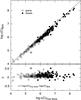 |
Fig. 2 Comparison of the carbon abundance determined in this work with those of B05. The open circles refer to giants, while the filled circles represent subgiants and dwarfs. The solid line is the one-to-one correlation and the dotted line represents a linear fit of the data. |
The carbon abundance ratio as a function of Teff is shown in Fig. 3. The decreasing [C/Fe] towards decreasing Teff for stars whose Teff are below 5000 K is expected, because the surface abundance of carbon of evolved giants may be deficient owing to the mixing processes including first dredge-up and extra-mixing (Cayrel et al. 2004; Lucatello et al. 2006; Aoki et al. 2007). For the giants with Teff lower than 5000 K, contamination of Si i 3905 Å by CH B-X band can be neglected. Excluding these low-temperature giants and the carbon enhanced stars ([C/Fe] > 1.0 dex (see Lucatello et al. 2006), the ⟨ [C/Fe] ⟩ = 0.33 ± 0.24 dex. If the carbon enhanced stars are accounted for, the average value is changed to 0.42 ± 0.44 dex, with larger dispersion. These values imply that the CH B-X band may affect the line profile of Si i 3905 Å for most of our sample stars, thus it is necessary to add CH B-X band in our line fitting.
4.2. Silicon
Our silicon abundance results are also listed in Table 3. The average value and standard deviation of the abundance ratios derived by these two lines are as follows: ⟨ [Si/Fe] 3905 ⟩ = 0.44 ± 0.39 (247 stars) and ⟨ [Si/Fe] 4103 ⟩ = 0.41 ± 0.42 (199 stars). Note that the stars for which only upper limits are available are not considered in these calculations.
The abundance discrepancy between Si3905 and Si4103 as a function of the C abundance and the stellar parameters is shown in Fig. 4. In this figure, only the stars that had both lines measured are used to make a comparison. The dashed lines in Fig. 4 present the average difference (0.06 dex) and 1σ scatter (±0.09 dex). In the upper panel there is no trend in Δ(=log ε(Si)3905 − log ε(Si)4103) vs. log ε(C). This reflects that the contamination with the CH B-X band has been eliminated in our final results.
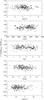 |
Fig. 4 Difference between the abundances of Si determined by the Si i 3905 and 4103 Å lines as a function of the C abundance and stellar parameters. The symbols are the same as in Fig. 2. The dashed lines show the average difference between these two lines and 1σ scatter. |
There is a small offset between the results derived from 3905 Å and those derived from the 4102.93 Å line. According to Shi et al. (2008), the 4102.93 Å line should yield a higher abundance if the log gf values of Garz (1973) are adopted (see Shi et al. 2008, Fig. 7). Our results show the contrary. As discussed above, the blend with CH lines is unlikely to be the reason. Moreover, most of the sample stars are very metal-poor, thus blends of other metal components can be neglected. From the panels of Fig. 4, the distribution of the difference shows a concentration around giants. This phenomenon may be explained by two reasons:
-
(1)
Lai et al. (2008) raised thehypothesis that strong lines would lead to higher abundancevalues than weak ones, especially in giants, if the T − τ relation of the adopted model atmosphere is shallower than that of true one. For most of the giants in our sample, the equivalent width (EW) of the line at 3905 Å (EW > 150 mÅ) is much larger than that of the 4103 Å line (EW < 120 mÅ), thus the larger derived abundance from the 3905 Å line and a slight increase of the difference towards decreasing Teff (see the second panel of Fig. 4) are reasonable;
-
(2)
the strong lines are sensitive to the micro-turbulence velocity. Twenty stars were used as a test: if the ξt value is increased 0.15 km s-1, the log ε(Si3905) will decrease by 0.11 dex, while the log ε(Si4103) only decreases by 0.04 dex. Hence, the determination of ξt may cause higher silicon abundances for the 3905 Å line.
Figure 4 also show that Δ decreases with increasing metallicity. This is probably an artifact that arises because the fact that the 4103 Å line is difficult to detected at low metallicity. In the comparison, stars in which only Si3905 can be detected are unavailable for this low-metallicity range.
The average of the Si abundance determined from Si3905 and Si4103 are taken to represent the final abundance. If only an upper limit can be derived from one line, we adopted the value derived from the other line. The average Si abundance ratio and its standard deviation are ⟨ [Si/Fe] ⟩ = 0.46 ± 0.20 (253 stars). This value is closed to the prediction in Goswami & Prantzos (2000) ( about 0.5 dex in the low-metallicity regime), while the value is 0.53–0.68 dex in the calculation of Kobayashi et al. (2006). The higher theoretical value is primarily caused by the adopted IMF in the models, because [α/Fe] is higher for larger stellar masses.
Considering the mixing effect in low-temperature giants and the accretion from a companion for the carbon enhanced metal-poor (CEMP) star, an average [Si/C] of 0.13 ± 0.21 in the range of 0 < [C/Fe] < 1 and Teff > 5000 K was estimated. In the predictions of (Woosley & Weaver 1995; Heger & Woosley 2002), [Si/C] is about 0.15 dex if the initial mass of the progenitor star was about 12–40 M⊙.
In the upper panel of Fig. 6 we show our results along with the results of previous LTE silicon abundance analyses. Most of these studies presented large scatter in [Si/Fe]. For instance, Ryan et al. (1996) showed that the star-to-star scatter increases towards decreasing [Fe/H], that is 0.11 for [Fe/H] > −1.5, 0.14 for −2.5 < [Fe/H] < −1.5, and 0.32 for [Fe/H] ≤ − 2.5. Preston et al. (2006) gave a star-to-star scatter of 0.22 for 24 giants( [Fe/H] < −2.0). In our NLTE results, the scatter of dwarfs is smaller (~0.13). Also, for the whole sample, the star-to-star scatter is close with the estimated uncertainties (~0.16), that is, 0.23 dex, 0.18 dex, and 0.16 dex in the metallicity ranges of [−4, −3], [−3, −2], and [−2, −1], respectively. In the lower panel of the same figure, our result shows a stronger correlation between [Si/Fe] and [Fe/H]. The slope of [Si/Fe] versus [Fe/H] found in our NLTE analysis is − 0.14 ([Si/Fe] = 0.15(±0.07) − 0.14(±0.03) × [Fe/H]), which is higher than the values found by most LTE results (e.g., –0.03 in McWilliam et al. 1995; –0.07 in Ryan et al. 1996; 0.03 in Honda et al. 2004; –0.06 in Preston et al. 2006, and so on). More details are discussed in Sect. 5.
5. Discussion and conclusions
5.1. Abundance correlations with stellar parameters
In Figs. 5 and 6 we show [Si/Fe] as a function of the stellar parameters. The abundance correlation with stellar parameters is discussed below.
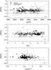 |
Fig. 5 Si abundance ratio as a function of stellar parameters. The arrows refer to upper limits; otherwise, the symbols are the same as in Fig. 2. The average error bar is shown in the lower right corner of each panel. The crosses are the results of Preston et al. (2006), while the open triangles are those of Lai et al. (2008). Besides, in the upper panel the dashed line, short dashed line, and dot-dashed line represent the least-square fits of the results of our observed data, Preston et al. (2006), and Lai et al. (2008), respectively. |
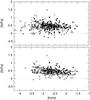 |
Fig. 6 Same as Fig. 5, but for [Si/Fe] vs. [Fe/H]. In the upper panel we compare our results with those of previous LTE analyses: McWilliam et al. (1995, pluses); Ryan et al. (1996, asteriks); Cayrel et al. (2004, open square); Honda et al. (2004, open diamonds); Aoki et al. (2005, filled square). In the lower panel the thick solid lines are 1-σ scatter, the short dashed lines crossing data points represent the fitting slope, and the dashed-dotted lines are the fitting uncertainties. |
Previous LTE silicon abundance analyses of metal-poor stars reported a correlation of [Si/Fe] with Teff (e.g. Preston et al. 2006; Lai et al. 2008), i.e., [Si/Fe] decreases with increasing temperature. In our results with NLTE correction, the phenomenon is not obvious. The slopes of these three data sources are listed below:
(1) this work:
[Si/Fe] =  ;
;
[Si/Fe] =  ;
;
(3) Lai et al. (2008):
[Si/Fe] =  .
.
Note that  .
.
These relation can be also seen in the upper panel of Fig. 5, in which our results are plotted along with previous LTE abundance analyses. The steep slope in [Si/Fe] versus Teff in previous studies is mainly caused by the low [Si/Fe] stars hotter than ~ 5500 K. The NLTE correction decreases with decreasing temperature. At higher Teff, the results with NLTE correction will become larger, which causes a higher silicon abundance than those of LTE and makes this slope much smaller. Therefore, our results support the conclusion of Shi et al. (2009) that NLTE effects can explain the temperature dependency of [Si/Fe]. Therefore, the increasing trend of [Si/Fe] with the declined Teff is diminished, if NLTE is considered in the abundance analysis of silicon.
Preston et al. (2006) concluded that there was no correlation between [Si/Fe] and log g, and our NLTE results also confirm this conclusion.
In the lower panel of Fig. 6, an increase of [Si/Fe] with decreasing [Fe/H] can be seen. Although Fe i is affected by significant NLTE effects for giants and very metal-poor stars (e.g. Teff = 5000 K, log g = 2.00, and [Fe/H] = −3.00, Mashonkina et al. 2010), the NLTE correction of Fe i leads only to small changes in our final [Si/Fe] results and the slope of [Si/Fe] vs. [Fe/H]. In the worst case, we find a NLTE correction for [Fe/H] of + 0.25 dex, corresponding to a change in [Si/Fe] of + 0.03 dex. Applying the corrections to our 22 very metal-poor giants ([Fe/H] < −3.0 dex) would lead a change of +0.02 in the slope of [Si/Fe] vs. [Fe/H]. In addition, the corrections for stellar granulation for Si and Fe are small (i.e., < 0.1 dex), and significant only for high-excitation potential lines in metal-deficient stars (Asplund 2005). Therefore, we conclude that the observed slope in Fig. 6 may not be the result of NLTE/3D effects.
Magnesium is also used as the tracer to discuss the metallicity dependence. In Fig. 7, [Si/Mg] is plotted against [Mg/H], where the magnesium abundances are taken from B05. A slope of [Si/Mg] vs. [Mg/H] can be noticed: [Si/Fe] = 0.02(±0.06) − 0.07(±0.03) × [Mg/H]. The NLTE effect of Mg may not be the reason which causes this tendency. This is because in the very recent NLTE study of Mg of Andrievsky et al. (2010), the NLTE results of Mg have the same evolution behaviour as the LTE ones, and the NLTE correction of Mg just enhances the abundance.
We discussed these trends in greater detail in Sect. 5.3.
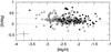 |
Fig. 7 [Si/Mg] as a function of [Mg/H]. The symbols are the same as in Fig. 5. The big triangles mark as Si-enhancement stars. Open triangles are giants, while filled ones are dwarfs. |
5.2. The outliers in our sample
We did not find any stars with a deficiency of Si (such as HE 1424−0241, Cohen et al. 2007). This star is at [Fe/H] ~ − 4 with an unusually low Si abundance, where [Si/Fe] = −1.01 and [Si/Mg] = −1.45. Cohen et al. (2008) speculated that this phenomenon may be the result of a chemically inhomogeneous ISM and that the star probably was enriched by a single SN. If that is the case, our results imply that our sample stars may not be formed in the gas that was contributed by ejecta from only one SN. This will be discussed further in Sect. 5.3.1.
On the other hand, we noticed five candidates with a large overabundance of silicon, [Si/Fe] are 1.47 dex, 0.99 dex, 1.10 dex, 1.01 dex, and 1.03 dex for HE 0308−1154, HE 1246−1344, HE 2314 − 1554, HE 0131−3953, and HE 1430−1123, respectively. The first three are giants and the other two are dwarfs. Only HE 0308−1154 whose [Si/Fe] is outside of the 3σ limit can be clearly considered as Si-enhancement (in our observed sample, [Si/Fe] is in Gaussian distribution, that is # = 253,μ = 0.46,σ = 0.20). To probe the nature of these stars, we investigate the abundance patterns of these stars, as derived by B05, and discuss them below.
Giants:
Two additional metal-deficient giants with large Si-enhancement are known:
-
(1)
CS29498 − 043 [Fe/H] = −3.75 dex, [C/Fe] = 1.90 dex, [Mg/Fe] = 1.81 dex, [Si/Fe] = 1.07 dex (Aoki et al. 2002);
-
(2)
CS22949 − 037 [Fe/H] = −3.79 dex, [C/Fe] = 1.05 dex, [Mg/Fe] = 1.22 dex, [Si/Fe] = 1.04 dex (Norris et al. 2001).
Both of them are CEMP stars with a large excess of α-elements.
However, in our study, the giants HE 0308−1154, HE 1246−1344, and HE 2314−1554 have otherwise “normal” abundance ratios. We checked the EW of two Si i lines of these three stars, and found that both EWs of these lines are larger than 100 mÅ, and the differences of derived abundance between Si i 3905 and 4103 are small. The incorrect “T − τ” relationship in model atmosphere (Lai et al. 2008) can result in an offset of 0.2 dex. This phenomena can be partially interpreted by the following hypothesis.
Dwarfs:
Previously, large excesses of Si were rarely found in dwarfs. The [Si/Fe] value of metal-deficient dwarfs determined by using Si i transitions in the red spectral region that are not affected by NLTE effects, are seldom higher than 0.6 dex (e.g. Stephens & Boesgaard 2002; Shi et al. 2009; Zhang et al. 2009), but these lines are difficult to detected at [Fe/H] < −2.0 dex. Even assuming a NLTE correction of + 0.2 dex for the [Si/Fe] values determined by Preston et al. (2006); Lai et al. (2008), where the Si abundance is derived from the 3905.93 Å line, none of the stars in their sample would be Si-enhanced by more than 0.75 dex.
The two Si-enhanced dwarfs, HE 0131−3953 and HE 1430−1123, are Ba-enhanced CEMP stars. Furthermore, HE 0131−3953 was identified as an s-II star2 by B05, and HE 1430−1123 has rather low [Sr/Ba] value of −1.58 dex, which is thought to be associated with the s-II stars. This star cannot be identified as a s-II star because of lacking abundance information for Eu (see more details in B05). Although mass transfer from a formerly more massive companion during its AGB phase might have caused the enhancements of C and Ba seen in these stars, this scenario does not provide an explanation for the Si-enhancements. Tsujimoto & Shigeyama (2003) suggested that it might be caused by pre-enrichment by subluminous SNe experiencing mixing and fallback. The fallback that occurred inside the Si layer in subluminous SNe can result in smaller abundances of elements heavier than Si and the enhancement of Si in these CEMP stars with regard to iron and the abundance ratio in the Sun.
5.3. Star-to-star scatter and mixing of the interstellar medium
The dispersion in the abundance ratios of metal-poor stars provides a measure of the chemical inhomogeneities in the star-forming gas, and hence of the mixing processes in the ISM. Audouze & Silk (1995) argued that increasing inhomogeneity is to be expected with decreasing metallicity as a result of the small number statistics of enriching events (i.e., SN II). This was also observed for a number of element ratios (Ryan et al. 1996; McWilliam 1997).
In the wake of these findings, Argast et al. (2000) derived the expected scatter for several abundance ratios, including [Si/Fe], as a function of metallicity. They predict a star-to-star scatter of ~ 0.4 dex in [Si/Fe] in the range of −4 < [Fe/H] < −3, at which the model ISM was essentially unmixed. The scatter reduces to ~ 0.25 dex in the range −3 < [Fe/H] < −2 owing to a gradually increased mixing. At [Fe/H] > −2.0, the scatter is around 0.2 dex, reaching typical levels of the observational uncertainties depending on the data quality.
In contrast, more recent studies have reported on a number of elements for which the scatter in the abundance ratios, like [Mg/Fe], are consistent with the observational uncertainties, all the way down to [Fe/H] ~ −3.5 (e.g., B05; Cohen et al. 2004; Arnone et al. 2005; Lai et al. 2008; Bonifacio et al. 2009). In the present study, the 1-σ scatter in [Si/Fe] is 0.23 dex, 0.18 dex, and 0.16 dex in the metallicity range [−4, −3], [−3, −2], and [−2, −1], respectively. Because the halo ISM should be well mixed at metallicities higher than −2.0 dex, as suggested by minimal mixing models like the one by Argast et al. (2000), the scatter of 0.16 dex can be considered as the observational error. If this is the case, the cosmic scatter is less than 0.15 dex in the full range −4 < [Fe/H] < −2, which is considerably smaller than what was predicted by Argast et al. (2000). It therefore seems that Si also belongs to the class of elements that show very little cosmic scatter. However, extreme outliers do also exist in [Si/Fe] (see Cohen et al. 2007). It is not entirely known which role these outliers play. Have they been formed out of gas enriched by SNe in a specific mass range, or are they “freak objects” formed under very particular circumstances? In the latter case, the measured surface abundances may not uniquely reflect common SN nucleosynthesis. We will discuss these questions in greater detail below.
5.3.1. Stochastic modelling of the chemical evolution of Si
In order to investigate the enrichment and amount of mixing in the early ISM, our large, homogeneous sample is compared with a stochastic model of the chemical evolution of Si. The statistics discussed here are based on a model that was originally developed by Karlsson (2005, 2006) and Karlsson et al. (2008). In this model, stars are assumed to form randomly within the system. They enrich their surroundings locally by ejecting heavy elements such as Si and Fe. The Fe yields used to calculate the metallicity distribution function (MDF) depicted in Fig. 8 are taken from Umeda & Nomoto (2002), and are nearly identical to the Fe-yields presented in Nomoto et al. (2006). The turbulent mixing of the ISM is modelled as a diffusion process in a way that each individual SN remnant continues to grow in time as
 (1)
(1)
where Vmix is the mixing volume and Dturb = 1.2 × 10⁻⁴ kpc Myr-1 is the turbulent diffusion coefficient. Here, σE, which is a measure of the initial size of the SN remnant as it merges with the ambient medium, is set to zero. The model used to calculate the MDF is nearly identical to model A in Karlsson (2005).
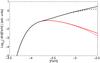 |
Fig. 8 Logarithm of the predicted metallicity distribution function (MDF). The quantity f is the fraction of stars that fall within each [Fe/H] bin (1 dex). The black, solid line shows the metal-poor tail of the predicted MDF of the Galactic halo, while the black, dashed line shows the predicted MDF of our observational sample. The red, solid and dashed lines denote the distribution of stars enriched by a single SN for the Galactic halo and the current sample, respectively. Below [Fe/H] ~ −3.8, the number of stars quickly goes to zero. |
The large number of stars in the present sample enables us to discuss outlier statistics. For example, what is the probability of finding an extreme Si-abundant star, similar to HE 1424 − 0241 (Cohen et al. 2007), in our sample? We shall make the simplifying assumption that stars with such extreme [Si/Fe] ratios can only occur if they were enriched by a single SN (Cohen et al. 2008) within a certain range of masses. Theoretically, the low Si-star may be enriched by two or more SNe, all within that same mass range, but this probability quickly goes to zero if the fraction of SNe within this range is ≲ 30%, or so. About 16% of all Galactic halo stars are found to have a metallicity below [Fe/H] = −2.5 (Carney et al. 1996). Assuming that stars enriched by one SN are predominantly found in this metallicity regime (see Fig. 8), the probability of finding a star enriched by a single SN in the Galactic halo is thus estimated to be p1,halo = 9 × 10⁻³, given the simulated metallicity distribution function (MDF) in Fig. 8.
Because our sample is biased against stars above [Fe/H] ~ −2.5, this must be accounted for if we seek to directly compare the observations with the model. A selection function of B − V = 0.7 was adopted (see Schörck et al. 2009, their Table 12). While stars enriched by one SN are hardly affected at all by this bias (i.e., they are mostly found below [Fe/H] = −2.5), the number of stars enriched by more than one SN is significantly smaller, by a factor of ~7. Consequently, the fraction of stars enriched by single SNe in the present observational sample is higher compared with the corresponding fraction of the Galactic halo (see Fig. 8). The biased fraction is estimated to be p1,bias = 6.1 × 10⁻².
The probability of finding exactly k stars with similarly extreme abundances like HE 1424 − 0241. In a sample of n stars is given by the binomial statistics B(n,k) = C(n,k)pkqn − k, where p is the probability of success, q = 1 − p and C(n,k) = n ! /k ! (n − k) ! . Given that only a fraction, fxtrm, of the stars enriched by a single SN may show an extreme abundance, the probability of finding such a star is therefore pxtrm = fxtrm p1,bias. The fraction fxtrm depends critically on the stellar yields and the IMF. Both parameters are uncertain, in particular in this extremely metal-poor regime.
5.3.2. Abundance ranges, dispersions, and outlier statistics
Including the low Si-star HE 1424−0241, the observed range in [Si/Fe] between this star and the mean of the sample is ~1.5 dex. The lowest 33% of this range will still keep us below [Si/Fe] = −0.5 (i.e., outside ~5σ of the current sample), which is ≥ 0.5 dex below the next lowest observed [Si/Fe] ratio at ~0. From current observations we are unable to estimate how big fxtrm is in this lower range. However, even though the theoretical yields do not predict these low values in [Si/Fe], we can estimate fxtrm by calculating the fraction of stars that falls within the lowest 33% of the corresponding theoretical range. This range, as predicted by the yield calculations of Heger & Woosley (2010), is reached by 7.5% of the massive stars within 10 − 40 M⊙, for a Salpeter IMF. The corresponding fraction using the yields by Nomoto et al. (2006) is 41.5%, in the mass range 13 − 40 M⊙. We will adopt a fiducial value of fxtrm = 0.15, and allow for a range of 0.05 ≤ fxtrm ≤ 0.45.
The probability of finding one or more stars (k ≥ 1) with a low [Si/Fe] in a sample of n = 253 stars can be expressed as B(n = 253,k ≥ 1) = 1 − (1 − pxtrm)n = 90.2%, for fxtrm = 0.15 and p1,bias = 6.1 × 10⁻². Within the range fxtrm = 0.05 − 0.45, the chance is B = 53.8 − 99.9%, with increasing B for increasing fxtrm. This is high, irrespective of the value of fxtrm. For fxtrm = 0.075, the chance is B = 68.7 ≃ 70%. Hence, the probability is high that at least one star with an extremely low [Si/Fe] would have been detected in the current sample. However, as noted in Sect. 5.2, there are no such stars in our sample. In this respect, our observations appear to be inconsistent with an inhomogeneous ISM in which the metal-poor stars in the Galactic halo were enriched only by a small number of SNe, as indicated by the presence of HE 1424−0241 at [Si/Fe] = −1.01. The star found by Cohen et al. (2007) have such a low [Si/Fe] and appears so detached from the rest of the halo stars, which all have [Si/Fe] ≳ 0, may suggest that its Si abundance is not (only) a result of enrichment by regular core collapse SNe (cf. Cohen et al. 2007). If this is the case, we should exclude it from the comparison between the observed and simulated star-to-star scatter. This view is also supported by the findings above that more like this stars would likely have been detected in our sample if this star were a “normal” outlier, enriched by a regular core collapse SN.
Below, we will exclude HE 1424 − 0241 from the discussion and only consider the sample stars presented here (Table 3). Consequently, the observed range in [Si/Fe] is significantly reduced, with a star-to-star scatter of σ = 0.22 below [Fe/H] = −3. As illustrated in the upper panel of Fig. 9, the observed 1-σ scatter is comparable with the theoretical dispersions expected from the yield ratio of Si-to-Fe over the mass range of core collapse SNe (the distributions in Fig. 9 are convolved with a Gaussian (σ = 0.14) to account for the random errors in the observations). The yield calculations by Nomoto et al. (2006) infer a dispersion of σ = 0.33 while the calculations by Heger & Woosley (2010) infer a dispersion of σ = 0.23, or σ = 0.27, if the full mass range 10 ≤ m/ℳ⊙ ≤ 100 is considered. Moreover, the observed range, [Si/Fe]max – [Si/Fe]min = 1.53, is larger than the expected theoretical range predicted by Heger & Woosley (2008, the observed range is larger in > 99.9% of the cases for n = 253 stars, assuming SN progenitor masses in the range 10 ≤ m/ℳ⊙ ≤ 40), while it is comparable with the one predicted by Nomoto et al. (2006), larger in 38% of the cases.
These are the maximum theoretical dispersions and ranges. In reality, we expect the stars enriched by a single SNe to be distributed over a range in [Fe/H]. In particular, a fraction of the stars below [Fe/H] = −3 are expected to be enriched by more than one SN. These stars are closer to the mean [Si/Fe] and the observed 1-σ dispersion below [Fe/H] = −3 (see Fig. 9, lower panel) is therefore expected to be lower than the dispersion of the yield ratio depicted in Fig. 9, upper panel. The lower panel of Fig. 9 shows a simulation in which the turbulent mixing is turned off (i.e., minimal mixing). The size (mixing volume) of the SN remnants is set to σE = 8.5 × 10⁻³, which corresponds to a mixing mass of 1 × 10⁵ ℳ⊙, for a particle density of 1 cm-3. The SN II yields are taken from Nomoto et al. (2006). Apart from the overall trend, which is shallower in the simulation, the 1-σ scatter in the metallicity three bins [−4, −3] , [−3, −2] , and [−2, −1] are found to be 0.23, 0.16, and 0.14, respectively, excluding the stars that are predominantly enriched by electron capture SNe (see below). This is significantly smaller than the scatter predicted by Argast et al. (2000) and closely agree with observations. Because we turned off the turbulent mixing in our simulations, the discrepancy between the two model results should predominantly be caused by differences in the adopted SN yields.
In conclusion, we cannot reject the possibility that the stars in our sample were formed in a chemically inhomogeneous ISM, solely based on the measurements of Si. Admittedly, our sample lacks extremely Si-deficient stars, but this may instead suggest that HE 1424 − 0241 is very atypical, and should not be included in the analysis. If this star was born with this low Si abundance, which reflects the nucleosynthesis of a rare SN, the early ISM must indeed have been highly inhomogeneous. Note that gas that low in Si will rapidly reach “chemical normality” as soon as SNe II enrich it. Low Si-stars would therefore be relatively uncommon. Moreover, the observed scatter increases faster with decreasing [Fe/H] than does the mean observational uncertainty of the stars (see Fig. 6, lower panel). This suggests that the scatter at the lowest metallicities has a small but non-negligible contribution from real abundance inhomogeneities in the early star-forming gas.
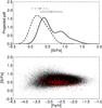 |
Fig. 9 Expected star-to-star scatter in [Si/Fe] for core collapse SNe. The top panel shows the expected maximum range in [Si/Fe] for stars enriched by single Type II SNe. The solid curve denotes the probability density function (PDF) assuming SN yields by Nomoto et al. (2006), while the dashed curve (SN mass range 10 ≤ m/ℳ⊙ ≤ 40) and the dotted curve (10 ≤ m/ℳ⊙ ≤ 100) denote the PDFs assuming yields by Heger & Woosley (2008). Each PDF is convolved with a Gaussian (σ = 0.14) to account for the observational uncertainty in [Si/Fe]. The corresponding 1-σ dispersions are shown as solid (σ = 0.33), dashed (σ = 0.23), and dotted (σ = 0.27) thin lines, centered at the respective mean of each distribution. The grey thin line at [Si/Fe] = 0.53 denotes the observational star-to-star scatter (σ = 0.22) below [Fe/H] = −3. The bottom panel shows the full (convolved) distribution of model stars (small black dots) in the [Fe/H] – [Si/Fe] plane. The observations are shown as red dots (upper limits are shown as triangles), for comparison. The star-to-star scatter below [Fe/H] = −3 in the simulation is σ ≃ 0.23. Note the small number of EMP stars below [Si/Fe] ~ 0. These stars have been partly enriched by electron capture SNe in the mass range 8 ≤ m/ℳ⊙ ≤ 10, which produce very small amounts of Si. The SN II (Fe-core collapse) yields are taken from Nomoto et al. (2006), while the electron capture SN yields are taken from Wanajo et al. (2009). |
5.3.3. Contribution from electron capture SNe
To find out the frequency of low-Si stars enriched by a rare type of SNe, we included the contribution of electron capture SNe, which have masses in the range 8 − 10 ℳ⊙. The electron capture SNe are believed to constitute a fraction of ~4−30% of all SNe (Poelarends et al. 2008; Wanajo et al. 2009, 2011). During the final stage of their evolution, these objects develop a degenerate O-Ne-Mg core and their structure and nucleosynthesis are distinctly different from the more massive Fe-core collapse SNe, including a very low Si yield (Wanajo et al. 2009). Assuming that all stars in the mass range 8 − 10 ℳ⊙ become electron capture SNe (i.e., 30% of all SNe, given a Salpeter IMF), the fraction of stars in the simulation with a [Si/Fe] < − 0.5 is pxtrm ≃ 1.55 × 10⁻³. This results in a probability of 32.4% of finding a low [Si/Fe] star in our sample. It is a relatively low probability, but not extremely low, and the possibility to find such a star in the combined sample of Galactic halo stars studied with detailed spectroscopy is non-negligible. The lower panel of Fig. 9 is truncated at [Si/Fe] = −0.5. Nevertheless, the few model stars below [Si/Fe] ~ 0 do have a small contribution from electron capture SNe.
Although the electron capture SNe indeed produce a low Si yield and the fraction of low-Si stars enriched by this type of SN is consistent with observations, the overall predicted abundance pattern (Wanajo et al. 2009) provides quite a poor fit to that observed in HE 1424 − 0241. The situation improves if a few per mille of ejecta of an Fe-core collapse SN areadded to the gas. However, the fit to the light elements Na, Mg, and Al is still poor. It is beyond the scope of this study to discuss the abundance pattern and possible origin of HE 1424 − 0241 in detail. The interested reader is directed to Cohen et al. (2007).
5.3.4. A note on trends and observed scatter
As discussed in Sect. 5.1 and the begining of Sect. 5.3, our results present not only a slope in [Si/Fe] with metallicity, but also a small cosmic scatter.
Trends as well as scatterss are affected by the star formation and mixing time scale of the ISM. Homogeneous chemical evolution models assume instantaneous mixing. In these models trends may in the most metal-poor regime arise from the progenitor mass dependence of the SN yields. A given abundance ratio, e.g., [Si/Fe], evolves with time, or metallicity, because the most massive, short-lived SNe have a different [Si/Fe] yield ratio from those of less massive, longer-lived SNe.
However, mixing is not instantaneous. In order to relax the assumption of unphysically short mixing time scales and still retain the small star-to-star scatter observed in a number of abundance ratios, Arnone et al. (2005) speculated that the cooling time scale of metal-poor gas may be long enough for the ISM to mix before subsequent generations of stars are able to form. However, because the star-forming gas in this scenario always has to be well mixed, this type of “global mixing” would have difficulties to explain any trends with metallicity like the one reported here (see also, e.g., Cayrel et al. 2004), unless these trends are a result of a metallicity-dependency of the SN yields. In the case of Si, the conclusion is ambiguous. Nomoto et al. (2006) predict a trend in [Si/Fe] with metallicity that goes in the right direction, although with a shallower slope than what is observed, while Chieffi & Limongi (2004) predict almost no trend, but with a very shallow slope in the opposite direction.
An alternative explanation for the small observed scatter without invoking an unphysically short mixing time scale is suggested by Bland-Hawthorn et al. (2010). They present a new stochastic chemical evolution model in which stars are formed in clusters, as is known to be the case in present-day star formation. In this scenario, the mixing initially only occurs on a local scale. However, as a result of stars being grouped together in clusters, the ejecta of ≥ 1 SNe are mixed together within each cluster, provided the clusters are massive enough to contain SNe. This may produce enough mixing to explain the observations of, e.g., [Mg/Fe], while the large scatter observed for a number of neutron-capture elements, e.g., [Ba/Fe] (Burris et al. 2000; François et al. 2007), can still be accounted for. This will be discussed in a forthcoming paper.
Karlsson & Gustafsson (2005) found trends with metallicity for certain abundance ratios, while the scatter stayed small at all metallicities, and, in particular cases, even decreased towards lower metallicity. These trends are an effect of the local enrichment in which different regions are enriched by SNe of different masses. A similar effect was noticed by Ryan et al. (1996). If the metal-poor star-forming gas were not very well mixed, trends like these are to be expected, depending on the SN yields. The very same SN mass dependence could in homogeneous models generate a trend with a different or even opposite slope to that in a stochastic, inhomogeneous model. Finally, a change in the IMF, e.g. from a top-heavy to a Salpeter-like IMF, may also possibly generate a trend with a non-zero slope. Clearly, to fully unravel the origins of the observed trends at low metallicities, a deeper understanding of the interplay between the mixing and cooling processes in the ISM is necessary (Karlsson et al. 2011). This knowledge must be incorporated in the modelling of chemical evolution.
Online material
Abundance results of carbon and silicon.
[A/B] = log (NA/NB) − log (NA/NB)⊙.
This kind of star is also called r + s star (Jonsell et al. 2006).
Acknowledgments
We thank Dr. J. R. Shi for useful suggestions and discussions on NLTE corrections. This work is supported by the NSFC under grant 10821061, by the National Basic Rsearch Program of China under grant 2007CB815103, and the Global Networks program of the University of Heidelberg. T.K. is funded by ARC FF grant 0776384 through the University of Sydney. T.K. is grateful to the Beecroft Institute for Particle Astrophysics and Cosmology for their hospitality. A.J.K. acknowledges support through grants by the Swedish Research Council (VR) and the Swedish National Space Board (SNSB). P.S.B. is a Royal Swedish Academy of Sciences Research Fellow supported by a grant from the Knut and Alice Wallenberg Foundation. P.S.B. also acknowledges additional support from the Swedish Research Council. A number of comments and suggestions by an anonymous referee helped improving the paper.
References
- Allen de Prieto, C., Lambert, D. L., & Asplund, M. 2002, ApJ, 573, L137 [NASA ADS] [CrossRef] [Google Scholar]
- Andrievsky, S. M., Spite, M., Korotin, S. A., et al. 2010, A&A, 509, A88 [NASA ADS] [CrossRef] [EDP Sciences] [Google Scholar]
- Anstee, S. D., & O’Mara, B. J. 1991, MNRAS, 253, 549 [Google Scholar]
- Anstee, S. D., & O’Mara, B. J. 1995, MNRAS, 276, 859 [NASA ADS] [CrossRef] [Google Scholar]
- Aoki, W., Norris, J. E., Ryan, S. G., Beers, T. C., & Ando, H. 2002, ApJ, 576, L141 [NASA ADS] [CrossRef] [Google Scholar]
- Aoki, W., Honda, S., Beers, T. C., et al. 2005, ApJ, 632, 611 [NASA ADS] [CrossRef] [Google Scholar]
- Aoki, W., Beers, T. C., Christlieb, N., et al. 2007, ApJ, 655, 492 [NASA ADS] [CrossRef] [Google Scholar]
- Argast, D., Samland, M., Gerhard, O. E., & Thielemann, F. 2000, A&A, 356, 873 [NASA ADS] [Google Scholar]
- Arnone, E., Ryan, S. G., Argast, D., Norris, J. E., & Beers, T. C. 2005, A&A, 430, 507 [NASA ADS] [CrossRef] [EDP Sciences] [Google Scholar]
- Asplund, M. 2005, ARA&A, 43, 481 [NASA ADS] [CrossRef] [Google Scholar]
- Audouze, J., & Silk, J. 1995, ApJ, 451, L49 [NASA ADS] [CrossRef] [Google Scholar]
- Barklem, P. S., Christlieb, N., Beers, T. C., et al. 2005, A&A, 439, 129 [NASA ADS] [CrossRef] [EDP Sciences] [Google Scholar]
- Beers, T. C., & Christlieb, N. 2005, ARA&A, 43, 531 [NASA ADS] [CrossRef] [Google Scholar]
- Beers, T. C., Rossi, S., Norris, J. E., Ryan, S. G., & Shefler, T. 1999, AJ, 117, 981 [NASA ADS] [CrossRef] [Google Scholar]
- Bland-Hawthorn, J., Karlsson, T., Sharma, S., Krumholz, M., & Silk, J. 2010, ApJ, 721, 582 [NASA ADS] [CrossRef] [Google Scholar]
- Bonifacio, P., Spite, M., Cayrel, R., et al. 2009, A&A, 501, 519 [NASA ADS] [CrossRef] [EDP Sciences] [Google Scholar]
- Burris, D. L., Pilachowski, C. A., Armandroff, T. E., et al. 2000, ApJ, 544, 302 [NASA ADS] [CrossRef] [Google Scholar]
- Carney, B. W., Laird, J. B., Latham, D. W., & Aguilar, L. A. 1996, AJ, 112, 668 [NASA ADS] [CrossRef] [Google Scholar]
- Cayrel, R., Depagne, E., Spite, M., et al. 2004, A&A, 416, 1117 [NASA ADS] [CrossRef] [EDP Sciences] [Google Scholar]
- Chieffi, A., & Limongi, M. 2004, ApJ, 608, 405 [NASA ADS] [CrossRef] [Google Scholar]
- Christlieb, N., Beers, T. C., Barklem, P. S., et al. 2004, A&A, 428, 1027 [NASA ADS] [CrossRef] [EDP Sciences] [Google Scholar]
- Cohen, J. G., Christlieb, N., McWilliam, A., et al. 2004, ApJ, 612, 1107 [NASA ADS] [CrossRef] [Google Scholar]
- Cohen, J. G., McWilliam, A., Christlieb, N., et al. 2007, ApJ, 659, L161 [NASA ADS] [CrossRef] [Google Scholar]
- Cohen, J. G., Christlieb, N., McWilliam, A., et al. 2008, ApJ, 672, 320 [NASA ADS] [CrossRef] [Google Scholar]
- François, P., Depagne, E., Hill, V., et al. 2007, A&A, 476, 935 [NASA ADS] [CrossRef] [EDP Sciences] [Google Scholar]
- Fuhrmann, K., Pfeiffer, M., Frank, C., Reetz, J., & Gehren, T. 1997, A&A, 323, 909 [NASA ADS] [Google Scholar]
- Garz, T. 1973, A&A, 26, 471 [NASA ADS] [Google Scholar]
- Goswami, A., & Prantzos, N. 2000, A&A, 359, 191 [NASA ADS] [Google Scholar]
- Grevesse, N., & Sauval, A. J. 1998, in Solar Composition and Its Evolution – From Core to Corona, ed. C. Fröhlich, M. C. E. Huber, S. K. Solanki, & R. von Steiger, 161 [Google Scholar]
- Grupp, F. 2004, A&A, 420, 289 [NASA ADS] [CrossRef] [EDP Sciences] [Google Scholar]
- Heger, A., & Woosley, S. E. 2002, ApJ, 567, 532 [NASA ADS] [CrossRef] [Google Scholar]
- Heger, A., & Woosley, S. E. 2010, ApJ, 724, 341 [NASA ADS] [CrossRef] [Google Scholar]
- Honda, S., Aoki, W., Kajino, T., et al. 2004, ApJ, 607, 474 [NASA ADS] [CrossRef] [Google Scholar]
- Jonsell, K., Barklem, P. S., Gustafsson, B., et al. 2006, A&A, 451, 651 [NASA ADS] [CrossRef] [EDP Sciences] [Google Scholar]
- Karlsson, T. 2005, A&A, 439, 93 [NASA ADS] [CrossRef] [EDP Sciences] [Google Scholar]
- Karlsson, T. 2006, ApJ, 641, L41 [NASA ADS] [CrossRef] [Google Scholar]
- Karlsson, T., & Gustafsson, B. 2005, A&A, 436, 879 [NASA ADS] [CrossRef] [EDP Sciences] [Google Scholar]
- Karlsson, T., Johnson, J. L., & Bromm, V. 2008, ApJ, 679, 6 [NASA ADS] [CrossRef] [Google Scholar]
- Karlsson, T., Bromm, V., & Bland-Hawthorn, J. 2011, Rev. Mod. Phys., submitted [arXiv:1101.4024] [Google Scholar]
- Kobayashi, C., Umeda, H., Nomoto, K., Tominaga, N., & Ohkubo, T. 2006, ApJ, 653, 1145 [NASA ADS] [CrossRef] [Google Scholar]
- Kurucz, R. 1993, Diatomic Molecular Data for Opacity Calculations, Kurucz CD-ROM, Cambridge, Mass.: Smithsonian Astrophysical Observatory, 15 [Google Scholar]
- Kurucz, R. L. 1992, Rev. Mex. Astron. Astrofis., 23, 45 [Google Scholar]
- Lai, D. K., Bolte, M., Johnson, J. A., et al. 2008, ApJ, 681, 1524 [NASA ADS] [CrossRef] [Google Scholar]
- Lucatello, S., Beers, T. C., Christlieb, N., et al. 2006, ApJ, 652, L37 [NASA ADS] [CrossRef] [Google Scholar]
- Mashonkina, L., Gehren, T., Shi, J., Korn, A., & Grupp, F. 2010, in IAU Symp., ed. K. Cunha, M. Spite, & B. Barbuy, 265, 197 [Google Scholar]
- McWilliam, A. 1997, ARA&A, 35, 503 [NASA ADS] [CrossRef] [Google Scholar]
- McWilliam, A., Preston, G. W., Sneden, C., & Searle, L. 1995, AJ, 109, 2757 [NASA ADS] [CrossRef] [Google Scholar]
- Nomoto, K., Tominaga, N., Umeda, H., Kobayashi, C., & Maeda, K. 2006, Nuclear Physics A, 777, 424 [Google Scholar]
- Norris, J. E., Ryan, S. G., & Beers, T. C. 2001, ApJ, 561, 1034 [NASA ADS] [CrossRef] [Google Scholar]
- Poelarends, A. J. T., Herwig, F., Langer, N., & Heger, A. 2008, ApJ, 675, 614 [NASA ADS] [CrossRef] [Google Scholar]
- Preston, G. W., Sneden, C., Thompson, I. B., Shectman, S. A., & Burley, G. S. 2006, AJ, 132, 85 [NASA ADS] [CrossRef] [Google Scholar]
- Reetz, J. K. 1991, Diploma Thesis, Universitä München [Google Scholar]
- Ryan, S. G., Norris, J. E., & Beers, T. C. 1996, ApJ, 471, 254 [NASA ADS] [CrossRef] [Google Scholar]
- Schörck, T., Christlieb, N., Cohen, J. G., et al. 2009, A&A, 507, 817 [NASA ADS] [CrossRef] [EDP Sciences] [Google Scholar]
- Shi, J. R., Gehren, T., Butler, K., Mashonkina, L. I., & Zhao, G. 2008, A&A, 486, 303 [NASA ADS] [CrossRef] [EDP Sciences] [Google Scholar]
- Shi, J. R., Gehren, T., Mashonkina, L., & Zhao, G. 2009, A&A, 503, 533 [NASA ADS] [CrossRef] [EDP Sciences] [Google Scholar]
- Stephens, A., & Boesgaard, A. M. 2002, AJ, 123, 1647 [NASA ADS] [CrossRef] [Google Scholar]
- Tsujimoto, T., & Shigeyama, T. 2003, ApJ, 584, L87 [NASA ADS] [CrossRef] [Google Scholar]
- Umeda, H., & Nomoto, K. 2002, ApJ, 565, 385 [NASA ADS] [CrossRef] [Google Scholar]
- Valenti, J. A., & Piskunov, N. 1996, A&AS, 118, 595 [NASA ADS] [CrossRef] [EDP Sciences] [Google Scholar]
- Wanajo, S., Janka, H., & Mueller, B. 2011, ApJ, 726, L15 [NASA ADS] [CrossRef] [Google Scholar]
- Wanajo, S., Nomoto, K., Janka, H., Kitaura, F. S., & Müller, B. 2009, ApJ, 695, 208 [NASA ADS] [CrossRef] [Google Scholar]
- Woosley, S. E., & Weaver, T. A. 1995, ApJS, 101, 181 [NASA ADS] [CrossRef] [Google Scholar]
- Zhang, L., Ishigaki, M., Aoki, W., Zhao, G., & Chiba, M. 2009, ApJ, 706, 1095 [NASA ADS] [CrossRef] [Google Scholar]
All Tables
Molecular line data for B-X system of the CH molecule near 3905 Å from Kurucz (1993).
All Figures
|
Fig. 1 Examples of spectral synthesis for six representative stars. The dots are the observational spectra, the solid lines are the best-fitting profile, and the dotted lines are the synthetic spectra with Si abundances of ± 0.15 dex with regard to the best fit, corresponding to less/more than 5% in the continuum. The listed parameters are Teff, log g, [Fe/H], and ξt, respectively. |
| In the text | |
|
Fig. 2 Comparison of the carbon abundance determined in this work with those of B05. The open circles refer to giants, while the filled circles represent subgiants and dwarfs. The solid line is the one-to-one correlation and the dotted line represents a linear fit of the data. |
| In the text | |
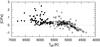 |
Fig. 3 [C/Fe] as a function of Teff. The symbols are the same as in Fig. 2. |
| In the text | |
|
Fig. 4 Difference between the abundances of Si determined by the Si i 3905 and 4103 Å lines as a function of the C abundance and stellar parameters. The symbols are the same as in Fig. 2. The dashed lines show the average difference between these two lines and 1σ scatter. |
| In the text | |
|
Fig. 5 Si abundance ratio as a function of stellar parameters. The arrows refer to upper limits; otherwise, the symbols are the same as in Fig. 2. The average error bar is shown in the lower right corner of each panel. The crosses are the results of Preston et al. (2006), while the open triangles are those of Lai et al. (2008). Besides, in the upper panel the dashed line, short dashed line, and dot-dashed line represent the least-square fits of the results of our observed data, Preston et al. (2006), and Lai et al. (2008), respectively. |
| In the text | |
|
Fig. 6 Same as Fig. 5, but for [Si/Fe] vs. [Fe/H]. In the upper panel we compare our results with those of previous LTE analyses: McWilliam et al. (1995, pluses); Ryan et al. (1996, asteriks); Cayrel et al. (2004, open square); Honda et al. (2004, open diamonds); Aoki et al. (2005, filled square). In the lower panel the thick solid lines are 1-σ scatter, the short dashed lines crossing data points represent the fitting slope, and the dashed-dotted lines are the fitting uncertainties. |
| In the text | |
|
Fig. 7 [Si/Mg] as a function of [Mg/H]. The symbols are the same as in Fig. 5. The big triangles mark as Si-enhancement stars. Open triangles are giants, while filled ones are dwarfs. |
| In the text | |
|
Fig. 8 Logarithm of the predicted metallicity distribution function (MDF). The quantity f is the fraction of stars that fall within each [Fe/H] bin (1 dex). The black, solid line shows the metal-poor tail of the predicted MDF of the Galactic halo, while the black, dashed line shows the predicted MDF of our observational sample. The red, solid and dashed lines denote the distribution of stars enriched by a single SN for the Galactic halo and the current sample, respectively. Below [Fe/H] ~ −3.8, the number of stars quickly goes to zero. |
| In the text | |
|
Fig. 9 Expected star-to-star scatter in [Si/Fe] for core collapse SNe. The top panel shows the expected maximum range in [Si/Fe] for stars enriched by single Type II SNe. The solid curve denotes the probability density function (PDF) assuming SN yields by Nomoto et al. (2006), while the dashed curve (SN mass range 10 ≤ m/ℳ⊙ ≤ 40) and the dotted curve (10 ≤ m/ℳ⊙ ≤ 100) denote the PDFs assuming yields by Heger & Woosley (2008). Each PDF is convolved with a Gaussian (σ = 0.14) to account for the observational uncertainty in [Si/Fe]. The corresponding 1-σ dispersions are shown as solid (σ = 0.33), dashed (σ = 0.23), and dotted (σ = 0.27) thin lines, centered at the respective mean of each distribution. The grey thin line at [Si/Fe] = 0.53 denotes the observational star-to-star scatter (σ = 0.22) below [Fe/H] = −3. The bottom panel shows the full (convolved) distribution of model stars (small black dots) in the [Fe/H] – [Si/Fe] plane. The observations are shown as red dots (upper limits are shown as triangles), for comparison. The star-to-star scatter below [Fe/H] = −3 in the simulation is σ ≃ 0.23. Note the small number of EMP stars below [Si/Fe] ~ 0. These stars have been partly enriched by electron capture SNe in the mass range 8 ≤ m/ℳ⊙ ≤ 10, which produce very small amounts of Si. The SN II (Fe-core collapse) yields are taken from Nomoto et al. (2006), while the electron capture SN yields are taken from Wanajo et al. (2009). |
| In the text | |
Current usage metrics show cumulative count of Article Views (full-text article views including HTML views, PDF and ePub downloads, according to the available data) and Abstracts Views on Vision4Press platform.
Data correspond to usage on the plateform after 2015. The current usage metrics is available 48-96 hours after online publication and is updated daily on week days.
Initial download of the metrics may take a while.