| Issue |
A&A
Volume 528, April 2011
|
|
|---|---|---|
| Article Number | A104 | |
| Number of page(s) | 8 | |
| Section | The Sun | |
| DOI | https://doi.org/10.1051/0004-6361/201014389 | |
| Published online | 09 March 2011 | |
Budget of energetic electrons during solar flares in the framework of magnetic reconnection
Astrophysikalisches Institut Potsdam,
An der Sternwarte 16,
14482
Potsdam,
Germany
e-mail: This email address is being protected from spambots. You need JavaScript enabled to view it.
Received:
9
March
2010
Accepted:
11
January
2011
Abstract
Context. Among other things, solar flares are accompanied by the production of energetic electrons as seen in the nonthermal radio and X-ray radiation of the Sun. Observations of the RHESSI satellite show that 1032−1036 nonthermal electrons are produced per second during flares. They are related to an energy flux in the range 1018−1022 W. These electrons play an important role, since they carry a substantial part of the energy released during a flare.
Aims. In which way so many electrons are accelerated up to high energies during a fraction of a second is still an open question. By means of radio and hard X-ray data, we investigate under which conditions this acceleration happens in the corona.
Methods. The flare is considered in the framework of magnetic reconnection. The conditions in the acceleration region in the corona are deduced by using the conservation of the total electron number and energy.
Results. In the inflow region of the magnetic reconnection site, there are typical electron number densities of about 2.07 × 109 cm-3 and magnetic fields of about 46 G. These are regions with high Alfvén speeds of about 2200 km s-1. Then, sufficient energetic electrons (as required by the RHESSI observations) are only generated if the plasma inflow towards the reconnection site has Alfvén-Mach numbers in the range 0.1−1, which can lead to a super-Alfvénic outflow with speeds up to 3100 km s-1.
Key words: acceleration of particles / Sun: flares / Sun: X-rays, gamma rays / Sun: radio radiation
© ESO, 2011
1. Introduction
A solar flare is basically defined as a sudden enhancement of the Sun’s emission of electromagnetic radiation, i.e. from the radio up to the γ-ray range (Priest 1981). During flares a large amount of stored magnetic field energy is suddenly released and transferred into a local heating of the coronal plasma, mass motions (e.g. jets), enhanced emission of electromagnetic radiation, and enhanced fluxes of energetic particles (e.g. electrons, protons, and heavy ions) (Heyvarts 1981). The energetic electrons play an important role, since they carry a substantial part of the flare released energy (Lin & Hudson 1971, 1976; Emslie et al. 2004).
The energetic electrons produced by a flare are travelling along the magnetic field lines towards the dense chromsphere, where they emit hard X-ray (HXR) radiation due to bremsstrahlung (Brown 1971). Nonthermal photon spectra, such as observed by the RHESSI spacecraft (Lin et al. 2002), can be converted into a differential injected nonthermal electron flux, from which the total flux Fe and kinetic power Pe of the accelerated electrons generated during a flare can be obtained. HXR observations have shown that these fluxes and powers can be extremely large (on the order of Fe = 1036 s-1 and Pe = 1022 W, see e.g. Holman et al. 2003; Emslie et al. 2004). It is still an open question how such a huge number of electrons is accelerated up to high energies within a fraction of a second during flares.
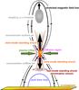 |
Fig. 1 Sketch of the reconnection process in the solar corona as described in Sect. 1. |
In solar physics, the flare is widely accepted in the framework of magnetic reconnection (see e.g. Shibata 1999). Figure 1 shows the corresponding scenario in a schematic manner. A prominence is destabilized by its photospheric footpoint motions leading to its rising up. This upward motion stretches the underlying magnetic field lines leading to the formation of a current sheet. If the current within this sheet exceeds a critical value, the resistivity is suddenly increased by plasma wave excitation owing to various instabilities (see e.g. Treumann & Baumjohann 1997). Then, magnetic reconnection can take place in the region of enhanced resistivity (also called diffusion region). Owing to the strong curvature of the magnetic field lines in the vicinity of the diffusion region, the slowly inflowing plasma shoots away from the reconnection site in oppositely directed jets (see Fig. 1), which are embedded between a pair of slow-mode standing shocks. Slow-mode shocks are accompanied by an increase in the density and temperature and a decrease in the magnetic field (Priest 1982). Thus, the plasma of these outflow jets has been heated by the slow-mode shocks (Cargill & Priest 1982). Such jets are apparently seen in the soft X-ray and/or EUV images of the Sun (Shibata et al. 1992, 1994; Wang et al. 2007). If the speed of this outflow jet is super-Alfvénic, a fast magnetosonic shock, also called termination shock can be established thanks to the deceleration of the jet during its penetration into the surrounding plasma. The appearance of such a shock is predicted in the numerical simulations by Forbes (1986) and Shibata et al. (1994). Aurass et al. (2002) and Aurass & Mann (2004) report on the signatures of such shocks in the solar radio burst radiation. This flare scenario is usually called the standard or CSHKP model (Carmichael 1964; Sturrock 1966; Hirayama 1974; Kopp & Pneumann 1976).
There are several mechanisms of electron acceleration within the flare scenario: one of them is the direct acceleration at the large scale DC electric field in the diffusion region (e.g. Holman 1985; Benz 1987; Litvinenko 2000). This process can even explain the acceleration of an electron up to high energies, but, the small spatial size of the diffusion region makes it impossible to provide a high production rate of energetic electrons (typically 1036 s-1 for large flares, see Fig. 3) as required by the observations. Therefore, Tsuneta & Naito (1998) proposed that the termination shock could be the source of energetic electrons, since it has a much greater real phase space than the diffusion region. This mechansim was studied in a quantitative manner by Mann et al. (2006, 2009). Other mechanisms are the acceleration at shock waves as a result of a blast wave and/or driven by a coronal mass ejection (Holman & Pesses 1983; Mann & Classen 1995; Mann & Klassen 2005), by stochastic acceleration via wave particle interaction in the highly turbulent flare region (Melrose 1994; Miller et al. 1996; Miteva & Mann 2007), and by acceleration in collapsing magnetic traps (Somov & Kosugi 1997; Karlicky & Kosugi 2004).
In Sect. 2, we describe the RHESSI hard X-ray observations that were used to constrain the typical nonthermal electron fluxes in solar flares. The plasma parameters in the flare region are derived from radio observations in Sect. 3. Adopting these parameters and considering the acceleration mechanism as a “black box”, the conditions of the plasma flowing into the reconnection site are derived under the requirement of compatibility with RHESSI observation in Sect. 4. Finally, the results are discussed in Sect. 5.
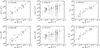 |
Fig. 2 Nonthermal electron fluxes Fe (upper row) and kinetic powers Pe (lower row) as a function of maximum GOES soft X-ray flux ISXR (i.e., GOES class; here ISXR = 10-6 W m-2 is a C1 flare, while ISXR = 10-4 W m-2 represents an X1 flare) for the 18 flares analyzed. The left column shows the maximum values of Fe and Pe, the middle column the mean values (with the error bars showing the whole range from minimum to maximum), and the right column shows the total flux Fe, tot and kinetic energy Ee of the electrons in the different flares. Also shown are linear fits using the bisector method (dashed line) and the slope α. |
2. Hard X-ray observations
To obtain representative electron flux and power values that are valid for both moderately sized and large flares, a sample of 18 flares ranging from GOES class C5.5 to X17.2 was analyzed (see Warmuth et al. 2009b). This sample includes five C-class flares, five M-class, seven X-class, and one flare greater than X10. The events in the sample were selected to cover some 2.5 decades of the (logarithmic) GOES class scale in a more or less uniform manner. It does not reflect solar flares in general – such a sample would be weighted heavily in favor of the smaller events.
We have obtained timeseries of RHESSI count rate spectra for all 18 events with time bins of 20 s (for 14 events) and 12 s (four events – in these cases the HXR flux was varying quickly, which suggested using smaller time bins to adequately capture the evolution). In all flares the impulsive phase, which is the main phase of electron acceleration, was fully observed, with the exception of the X17.2 flare of 2003 Oct. 28, where RHESSI observations started only after the main peak of the impulsive phase. This flare is nevertheless included as an example of an extremely energetic event.
For deriving the spectra we used only front detector 4, which has the best energy resolution and should therefore reveal all the features in the flare spectra most clearly. Using the OSPEX software package of the RHESSI analysis tools, spectral models of an isothermal component plus a nonthermal thick-target bremsstrahlung component (Brown 1971) were folded through the full detector response matrix and forward-fitted to the background-subtracted count rate spectra (cf. Holman et al. 2003). The spectra were corrected for pulse pileup and decimation (see Smith et al. 2002), as well as for photospheric albedo (see Kontar et al. 2006). Using a single detector allowed us to apply the advanced correction methods for the pulse pileup and gain offset provided by OSPEX (see also Warmuth et al. 2009a). The energy bin width was 1/3 keV below 15 keV, 1 keV to 50 keV, 5 keV up to 100 keV, and 10 keV above that.
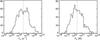 |
Fig. 3 Distribution of the flux Fe and related power Pe of nonthermal electrons produced during a sample of 18 flares. The median values are depicted as a dotted line in both cases. |
With regard to nonthermal electrons, these fits yield the total flux Fe, spectral indices δL and δH below and above the break energy EB, and low-energy cutoff ELC of the injected nonthermal electron flux. The high-energy cutoff was not fitted since it is usually masked by the background. By integrating the differential flux over energy, one obtains the total kinetic power Pe of the accelerated electrons. These fits usually yield only an upper limit for the low-energy cutoff, since the real one is often masked by the thermal component. Therefore, the nonthermal fluxes and power deduced are only lower limits.
In this manner, a total of 1142 spectra that had a detectable nonthermal component were fitted. Figure 2 shows how the electron fluxes Fe (upper row) and kinetic powers Pe (lower row) scale with GOES class. Also shown are linear fits to the logarithms of the data obtained with the linear least-squares bisector method (cf. Isobe et al. 1990) and the slope index α. The sample covers 2.5 decades of the GOES peak flux scale in a nearly uniform manner. The left column shows the peak values of Fe and Pe for the 18 flares. It is immediately evident that the peak values are systematically higher for the larger flares. The middle column depicts the mean values for Fe and Pe (dots), as well as the whole range from maximum to minimum values (error bars) in each event. Just like the peak values, the mean values grow with rising GOES class, albeit more slowly. The minimum values do not show such systematic behavior, but instead tend to be scattered in the range of 1033–1034 s-1 in terms of flux and 1019–1020 W in terms of power. This behavior is the consequence of the detection threshold for the nonthermal component due to the background and the masking of the low-energy cutoff by the thermal component. Finally, the right column shows the total flux Fe, tot and kinetic energy Ee (obtained by integrating Fe and Pe over time) for all flares. Again, both Fe, tot and Ee are correlated well with the peak GOES flux. These total values rise more steeply with GOES class (i.e., have a higher α) than the mean values. This reflects that larger flares also tend to have a longer impulsive phase.
The corresponding distributions of Fe and Pe are plotted in Fig. 3. Both Fe and Pe cover the ranges 3 × 1032–3 × 1036 s-1 and 3 × 10¹⁸–3 × 10²² W, respectively. The medians of theses distributions (dotted lines in Fig. 3) are 3.5 × 1034 s-1 and 2.2 × 10²⁰ W. A comparison with Fig. 2 shows that these values correspond to the peak of a mid-C-class flare or to the average Fe and Pe in a small M-class flare. In the following, we refer to this case as a moderate flare. Furthermore, we also consider the scenario of strong (i.e. X-class) flares. In order to obtain a representative value for Fe and Pe, only the part of the distribution where Fe > 1036 s-1 is evaluated. Again taking the medians, we obtain Fe = 1.5 × 1036 s-1 and Pe = 9.9 × 10²¹ W, which corresponds to the peak of a mid-X-class flare. Henceforth, this case will be referred to as the large flare. The mean energy of the energetic electrons estimated by Pe/Fe are the same, namely about 40 keV, for both moderate and large flares.
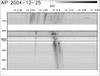 |
Fig. 4 Dynamic solar radio spectrum with a group of type III and reverse drifting bursts. It was recorded by the radio spectralpolarimeter (Mann et al. 1992) of the Astrophysical Institute Potsdam (Germany). For example, pairs of forward and reverse drift bursts appear at 230 MHz at 12:03 UT. |
3. Plasma parameters in the flare region
The standard model is also supported by radio observations. During solar flares, so-called pairs of forward and reverse drift bursts occur in dynamic spectra of the solar radio radiation. An example is shown in Fig. 4. Roughly at 12:03 UT, these features appear as a pair of stripes of enhanced radio emission simultaneously starting near the same frequency (e.g. at 230 MHz in Fig. 4) and, subsequently, rapidly drifting towards both higher and lower frequencies.
Generally, the solar radio radiation in the m- and dm-range is considered to be plasma emission (Melrose 1985); i.e., the radio waves are emitted near the local electron plasma frequency and/or its harmonics. Since the electron plasma frequency is proportional to the square root of the electron number density, the radio waves with higher and lower frequencies are emitted from the low and high corona, respectively, due to the gravitationally stratified solar atmosphere. If a radio source is moving upwards in the corona, its motion would appear as a drift towards lower frequencies in the dynamic radio spectrum.
As also seen in Fig. 4, the gaps between the starting frequencies of the forward and reverse drifting branches of these pairs are a few MHz (Aschwanden et al. 1995b). As a result, the pairs of forward and reverse drift bursts are regarded as the radio signature of electron beams simultaneously generated near the same region in the corona and, subsequently, travelling along the magnetic field lines towards the lower and higher corona. In the framework of the standard model, the frequency at which these pairs start in the dynamic radio spectrum (i.e. ≈230 MHz for the example shown in Fig. 4) gives the electron plasma frequency at the X-point (i.e. diffusion region in Fig. 4) of the magnetic reconnection. Of course, the density in the diffusion region is enhanced, but its spatial extension is relatively short, a few Mm (Aschwanden et al. 1995b). In addition, these pairs are observed over a broad frequency range (see Fig. 4), so the associated electron beams must propagate along well ordered magnetic field lines, i.e. mainly in an uncompressed region. Because of these arguments, it is justified to deduce the electron number density in the inflow region at the height of the X-point from staring frequencies of the pairs of forward and reversed drift bursts.
To relate the emission frequency to a height in the corona, a fourfold (i.e.
α = 4) Newkirk (1961) density
model 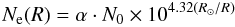 (1)(N0 = 4.2 × 104 cm-3;
R, distance from the center of the Sun; R⊙,
radius of the Sun) is adopted as an appropriate one above active regions (Koutchmy 1994). According to this model, the maximum electron
number density at the bottom of the corona (i.e.
R = R⊙) is
3.51 × 109 cm-3 corresponding to an electron plasma frequency of
532 MHz.
(1)(N0 = 4.2 × 104 cm-3;
R, distance from the center of the Sun; R⊙,
radius of the Sun) is adopted as an appropriate one above active regions (Koutchmy 1994). According to this model, the maximum electron
number density at the bottom of the corona (i.e.
R = R⊙) is
3.51 × 109 cm-3 corresponding to an electron plasma frequency of
532 MHz.
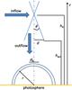 |
Fig. 5 Geometry of the reconnection region in the framework of the scenario presented in Fig. 1. |
A statistical analysis by Aschwanden et al. (1995b)
of a sample of 30 pairs of forward and reverse drift bursts shows that the radio signatures
of the X-points of the reconnection appear in the range 272–955 MHz. Now, all of them below
and above 532 MHz are considered to be generated by fundamental and harmonic emission,
respectively. Then, the mean frequency of radio signature of the X-point is at 360 MHz with
a standard deviation of 58 MHz (i.e. 16%) for the above-mentioned sample. It corresponds to
an electron number density of 1.61 × 109 cm-3. According to the
four-fold Newkirk (1961) density model (see Eq. (1))
the height of this frequency is located at 60 Mm, i.e.
hX = 60 Mm in Fig. 5. At
this height, a magnetic field of 20 G is expected according to the model by Dulk &
McLean (1978), i.e.,
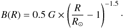 (2)This model describes the
radial behavior of the magnetic field above active regions in a rough sense.
(2)This model describes the
radial behavior of the magnetic field above active regions in a rough sense.
To determine the height of the acceleration region, Aschwanden et al. (1995a,b, 1996a,b,c)
introduced the method of time-of-flight (TOF) measurements. Here, the electrons are thought
to be accelerated at a height hacc in the corona and travel
along the magnetic field line towards the dense chromosphere, where they are stopped and
emit hard X-ray radiation via bremsstrahlung (Brown 1971). These studies provide a relation of
L′/s = 1.5 in a
statistical sense between the TOF distance L′ and the loop half
length s = π·r/2
(r, loop radius). The quantity L′ is actually
the length of the magnetic field line between the acceleration region and its footpoint in
the chromosphere. Aschwanden (2002) modeled such a
field line by a composition of two cirular segments with opposite curvature. Then, one gets
the relationship (see Eq. (4) in Aschwanden 2002)
![Mathematical equation: \begin{equation} \frac{L'}{r} = \frac{1}{2} \left(1 + \frac{h_{\rm acc}^{2}}{r^{2}}\right) \cdot \arctan \left(\frac{2 \cdot \frac{h_{\rm acc}}{r}} {\left[ \left(\frac{h_{\rm acc}}{r}\right)^{2}-1\right]}\right) \end{equation}](/articles/aa/full_html/2011/04/aa14389-10/aa14389-10-eq55.png) (3)between
the distance L′, the height of the acceleration region
hacc, and the loop radius r. For a typical
loop radius r = 10 Mm (see Fig. 12 in Aschwanden 2002) and
L′/r = 2.36 (because of
L′/s = 1.5) in the sense
of a mean value (Aschwanden 2002), the height of the
acceleration region can be determined as hacc = 20 Mm. The
location of the acceleration site is well below the height of the X-point (see Figs. 1 and 5). That should
be expected in the framework of the reconnection flare scenario as described in Sect. 1 At
the height of 20 Mm, an electron number density
Ne = 2.66 × 109 cm-3 and a magnetic
field of B = 104 G are found according to Eqs. (1) and (2).
(3)between
the distance L′, the height of the acceleration region
hacc, and the loop radius r. For a typical
loop radius r = 10 Mm (see Fig. 12 in Aschwanden 2002) and
L′/r = 2.36 (because of
L′/s = 1.5) in the sense
of a mean value (Aschwanden 2002), the height of the
acceleration region can be determined as hacc = 20 Mm. The
location of the acceleration site is well below the height of the X-point (see Figs. 1 and 5). That should
be expected in the framework of the reconnection flare scenario as described in Sect. 1 At
the height of 20 Mm, an electron number density
Ne = 2.66 × 109 cm-3 and a magnetic
field of B = 104 G are found according to Eqs. (1) and (2).
Finally, it is emphasized, that all these values of the plasma parameters and heights vary from event to event, so they should be regarded as mean values in the statistical sense; i.e., the deviations should be regarded as about 20%, since, for instance, the frequency of the X-point is fluctuating around 360 MHz with a typical deviation of 16%.
4. Budget of energetic electrons
In the framework of the flare scenario introduced in Sect. 1 (see Fig. 1), the plasma is laterally inflowing towards the reconnection region, then, it is pushed away from the reconnection site into the surrounding corona. The geometry of the reconnection region is drawn in Fig. 5. Here, the X-point of magnetic reconnection is considered to be located at hX = 60 Mm. The acceleration occurs at a height of hacc = 20 Mm. Since loops have typical radii of 10 Mm in the sense of a mean value (Aschwanden 2002), the height hacc is about 10 Mm above the top of the loop assuming the loop as a semi-circle. Then, the inflow region can be considered in the height range between hacc and hX. There, the electron number density varies in the ranges 2.66–1.61 × 109 cm-3 and the magnetic field of 104−20 G. Taking the geometric means, an electron number density Ne, in = 2.07 × 109 cm-3 and a magnetic field Bin = 46 G are chosen for typical values in the inflow region. That results in a ratio of ωpe/ωce = 3.2 between the electron plasma frequency ωpe = (4πe2Ne/me)1/2 and the electron gyrofrequency ωce = eB/mec and an Alfvén speed of vA = B/(4πmpNe)1/2 = 2200 km s-1 (e, elementary charge; me, electron mass; mp, proton mass; c, velocity of light) there, respectively.
The electron flux flowing towards the reconnection site is given by
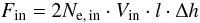 (4)with the inflow velocity
Vin and
Δh = hX − hacc,
where Ne, in denotes the electron number
density in the inflow region. The factor 2 appears in front of the righthand side of
Eq. (4), since the inflow comes from both sides of the reconnection site. The letter
l denotes the longitudinal extension of the reconnection region. Since
the plasma inflow is going towards the slow-mode standing shocks (see Fig. 1), Vin must be lower than the
local Alfvén speed, i.e.
Vin < vA, in
(Priest 1982). Then, the inflowing energy flux is
defined by
(4)with the inflow velocity
Vin and
Δh = hX − hacc,
where Ne, in denotes the electron number
density in the inflow region. The factor 2 appears in front of the righthand side of
Eq. (4), since the inflow comes from both sides of the reconnection site. The letter
l denotes the longitudinal extension of the reconnection region. Since
the plasma inflow is going towards the slow-mode standing shocks (see Fig. 1), Vin must be lower than the
local Alfvén speed, i.e.
Vin < vA, in
(Priest 1982). Then, the inflowing energy flux is
defined by  (5)In the inflow region, the
energy density win consists of the energy density of the
magnetic field
(5)In the inflow region, the
energy density win consists of the energy density of the
magnetic field  , the thermal energy density
wtherm = 3Ne, inkBTin
(kB, Boltzmann’s constant; Tin,
temperature in the inflow region; Bin, magnetic field in the
inflow region), and the kinetic energy of the inflowing plasma
, the thermal energy density
wtherm = 3Ne, inkBTin
(kB, Boltzmann’s constant; Tin,
temperature in the inflow region; Bin, magnetic field in the
inflow region), and the kinetic energy of the inflowing plasma
 ; i.e.;
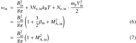 with
the plasma beta
βin = 16πNe, inkBT/B2
as the ratio between the total thermal and magnetic pressure and the Alfvén-Mach number
MA, in = Vin/vA, in
of the inflow. There, the Alfvén speed is defined by
vA, in = Bin/(4πNe, inmp)1/2.
Here, quasi-neutrality of the coronal plasma has been assumed. The Newkirk (1961) density model (see Eq. (1)) agrees with a
barometric height formula with a temperature of 1.4 MK (Mann et al. 1999). Adopting this value as the usual temperature of the corona, the
plasma beta can be determined to βin = 9.5 × 10⁻³ in
the inflow region. Because of βin ≪ 1, Eq. (6) reduces to
Eq. (7).
with
the plasma beta
βin = 16πNe, inkBT/B2
as the ratio between the total thermal and magnetic pressure and the Alfvén-Mach number
MA, in = Vin/vA, in
of the inflow. There, the Alfvén speed is defined by
vA, in = Bin/(4πNe, inmp)1/2.
Here, quasi-neutrality of the coronal plasma has been assumed. The Newkirk (1961) density model (see Eq. (1)) agrees with a
barometric height formula with a temperature of 1.4 MK (Mann et al. 1999). Adopting this value as the usual temperature of the corona, the
plasma beta can be determined to βin = 9.5 × 10⁻³ in
the inflow region. Because of βin ≪ 1, Eq. (6) reduces to
Eq. (7).
Since the hard X-ray sources have typical diameters of
dHXR = 10 Mm (see e.g. Warmuth et al. 2007, 2009b), l
as the longitudinal extension of the reconnection site is considered to be
l ≈ dHXR = 10 Mm. Of course, the flare
ribbons are usually much longer. But, since we are interested in studying the generation of
energetic electrons producing the hard X-ray emission, this choice of l
seems to be appropriate. For Δh,
Δh = hX − hacc = 40 Mm
is taken. Inserting these values and the plasma parameters of the inflow region as
introduced above into Eqs. (4), (5), and (7), one gets
 (8)and
 (9)with
Vin = MA, in ·vA, in
and vA, in = 2200 km s-1.
(9)with
Vin = MA, in ·vA, in
and vA, in = 2200 km s-1.
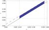 |
Fig. 6 The relationship between ϵ and ν for moderate flares. Here, the ϵth and νth part of the inflowing energy and electron number density are tranferred into the nonthermal electrons. The long dashed and full line represent ϵ = 1.55ν and ϵ = 0.78ν according to Eq. (21) for MA, in = 0.015 and 1, respectively. The dashed lines represent the relationships of Eqs. (18) and (19). |
Now, it is assumed that the ν-th part of the inflowing electrons and the
ϵ-th part of the inflowing energy is finally transfered into the
nonthermal electrons; i.e.,  (10)and
 (11)with
ν,ϵ ≤ 1. By means of Eqs. (8)–(11), one obtains
(11)with
ν,ϵ ≤ 1. By means of Eqs. (8)–(11), one obtains
 (12)and
 (13)Using
Fe = 3.5 × 1034 s-1 and
Pe = 2.2 × 10²⁰ W as typical values for moderate
flares as discussed above (see Sect. 1), Eqs. (12) and (13) result in
(13)Using
Fe = 3.5 × 1034 s-1 and
Pe = 2.2 × 10²⁰ W as typical values for moderate
flares as discussed above (see Sect. 1), Eqs. (12) and (13) result in
 (14)and
 (15)leading
to
(15)leading
to  (16)and
 (17)respectively, because of
ν < 1 and
MA, in < 1. Since
both relationships of Eqs. (16) and (17) must be fulfilled simultaneously, the quantities
ν, ϵ, and
MA, in must finally satisfy the
relationships
(17)respectively, because of
ν < 1 and
MA, in < 1. Since
both relationships of Eqs. (16) and (17) must be fulfilled simultaneously, the quantities
ν, ϵ, and
MA, in must finally satisfy the
relationships  (18)
(18) (19)
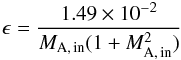
(19) (20)(see Fig. 6). The division of Eq. (15) by Eq. (14) provides
 (21)It leads to
ϵ = 1.55ν and
ϵ = 0.78ν as drawn in Fig. 6 for the case MA, in = 0.015 and
1, respectively. According to Eqs. (18), ν = 0.08 can be considered as a
typical value in the sense of a geometric mean. That leads to
MA, in = 0.12 and ϵ =
0.12 according to Eqs. (14) and (15). These values can be regarded as typical ones for
moderate flares.
(21)It leads to
ϵ = 1.55ν and
ϵ = 0.78ν as drawn in Fig. 6 for the case MA, in = 0.015 and
1, respectively. According to Eqs. (18), ν = 0.08 can be considered as a
typical value in the sense of a geometric mean. That leads to
MA, in = 0.12 and ϵ =
0.12 according to Eqs. (14) and (15). These values can be regarded as typical ones for
moderate flares.
For large flares, Fe = 1.5 × 1036 s-1 and
Pe = 9.9 × 10²¹ W (see discussion in Sect. 1) have
to be chosen in Eqs. (12) and (13). Following the same procedure as above, one gets
 (22)and
 (23)leading
to the relationship
(23)leading
to the relationship  (24)
(24) (25)
(25) (26)The division of Eq. (23)
by Eq. (22) provides
(26)The division of Eq. (23)
by Eq. (22) provides  (27)leading
to ϵ = 1.16ν and
ϵ = 0.82ν (see Fig. 7) for the cases MA, in = 0.53 and
1, respectively. For large flares, ν = 0.56 (as a geometric mean of the
boundaries given in Eq. (24)), MA, in = 0.73,
and ϵ = 0.60 according to Eqs. (22) and (23) are typical values for these
quantities. The values of ϵ and ν, which are compatible
with the RHESSI observations, are located in the shaded regions in
Figs. 6 and 7.
(27)leading
to ϵ = 1.16ν and
ϵ = 0.82ν (see Fig. 7) for the cases MA, in = 0.53 and
1, respectively. For large flares, ν = 0.56 (as a geometric mean of the
boundaries given in Eq. (24)), MA, in = 0.73,
and ϵ = 0.60 according to Eqs. (22) and (23) are typical values for these
quantities. The values of ϵ and ν, which are compatible
with the RHESSI observations, are located in the shaded regions in
Figs. 6 and 7.
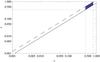 |
Fig. 7 The relationship between ϵ and ν for large flares, i.e. ϵ = 1.16ν (long dashed line) and ϵ = 0.82ν (full line) according to Eq. (27) for MA, in = 0.53 and 1, respectively. The dashed lines represent the relationships of Eqs. (24) and (25). |
According to Fig. 5, the conservation of the electron
and energy flux can be written as  (28)and
 (29)with
win and
(29)with
win and
 (30)as
the energy density in the inflow (see Eq. (6)) and outflow region, respectively (see e.g.
Baumjohann & Treumann 1997). Here,
Ne, out, Bout,
Tout and Vout denote the electron
number density, magnetic field, temperature, and flow speed in the outflow region,
respectively. Taking Eq. (28) and βin ≪ 1 into account, Eq. (29)
provides
(30)as
the energy density in the inflow (see Eq. (6)) and outflow region, respectively (see e.g.
Baumjohann & Treumann 1997). Here,
Ne, out, Bout,
Tout and Vout denote the electron
number density, magnetic field, temperature, and flow speed in the outflow region,
respectively. Taking Eq. (28) and βin ≪ 1 into account, Eq. (29)
provides  (31)with
vA, in as the Alfvén speed in the inflow
region. Because of MA, in ≤ 1 in the case of
slow shocks, Eq. (30) results in the well-known relationship
Vout ≤ 21/2vA, in.
According to the deduced plasma parameters in the inflow region, i.e.
vA, in = 2200 km s-1, one gets
an upper limit for the outflow speed
Vout ≤ 3100 km s-1. To evaluate whether the outflow
speed Vout is super-Alfvénic or not,
Vout must be normalized to the Alfvén speed in the outflow
region. It is given by
vA, out = Bout/(4πNe, outmp)1/2.
Then, one finds
(31)with
vA, in as the Alfvén speed in the inflow
region. Because of MA, in ≤ 1 in the case of
slow shocks, Eq. (30) results in the well-known relationship
Vout ≤ 21/2vA, in.
According to the deduced plasma parameters in the inflow region, i.e.
vA, in = 2200 km s-1, one gets
an upper limit for the outflow speed
Vout ≤ 3100 km s-1. To evaluate whether the outflow
speed Vout is super-Alfvénic or not,
Vout must be normalized to the Alfvén speed in the outflow
region. It is given by
vA, out = Bout/(4πNe, outmp)1/2.
Then, one finds  (32)Since
Ne, out/Ne, in >
1 and
Bout/Bin <
1 in the case of slow shocks (Priest 1982), the
righthand side of Eq. (32) is always greater than 1. As a result, it is possible that the
outflow becomes super-Alfvénic. The strongest slow shock is the so-called switch-off
shock. It appears for
MA, in → cosϑ ≤ 1. In this
case,
Bout/Bin = 1/cosϑ
with ϑ as the angle between the shock normal and the upstream magnetic
field; i.e., the magnetic field in the inflow region. Then,
Ne, out/Ne, in
varies between 4 and 2.5 as the angle ϑ is running from 0° to
90° (Priest 1982). Consequently, if the
slow shock becomes a switch-off one and nearly perpendicular, then, the
condition that the outflow becomes super-Alfvénic is fulfilled in the best way.
(32)Since
Ne, out/Ne, in >
1 and
Bout/Bin <
1 in the case of slow shocks (Priest 1982), the
righthand side of Eq. (32) is always greater than 1. As a result, it is possible that the
outflow becomes super-Alfvénic. The strongest slow shock is the so-called switch-off
shock. It appears for
MA, in → cosϑ ≤ 1. In this
case,
Bout/Bin = 1/cosϑ
with ϑ as the angle between the shock normal and the upstream magnetic
field; i.e., the magnetic field in the inflow region. Then,
Ne, out/Ne, in
varies between 4 and 2.5 as the angle ϑ is running from 0° to
90° (Priest 1982). Consequently, if the
slow shock becomes a switch-off one and nearly perpendicular, then, the
condition that the outflow becomes super-Alfvénic is fulfilled in the best way.
5. Summary
After adopting the magnetic reconnection as a flare scenario as described in Sect. 1 (see also Fig. 1), the plasma parameters, where the electron acceleration takes place, can be deduced from radio observations and time-of-flight measurements by BATSE (Burst and Transient Source Experiment) aboard the Compton Gamma Ray Observatory. As described in Sect. 2, typical electron number densities of about 2.07 × 109 cm-3 and magnetic field strengths of about 46 G are found in the inflow region located at a height of ≈40 Mm above the photopshere. These parameters lead to a ratio between the electron plasma frequency and the electron cyclotron frequency ωpe/ωce = 3.2 and to an Alfvén speed of about 2200 km s-1. This value of ωpe/ωce is relatively low in comparison to other coronal regions, where this ratio is in the range 10–40 (Mann et al. 2003; Warmuth & Mann 2005).
If this scenario is adopted as true, the flux and power of energetic electrons as observed by RHESSI during moderate flares can only be provided if ≈8% of the inflowing electrons are finally accelerated. Then, they have about 12% of the total energy incoming towards the flare region. That only happens if the inflow speed of plasma is about 260 km s-1.
In the special case of large flares, a major part (≈60%) of the incoming electrons are accelerated up to high energies >20 keV. They get a substantial part (≈60%) of the energy transfered during a large flare. That confirms in another way the observational result by Lin & Hudson (1971, 1976) and Emslie et al. (2004) that the energetic electrons carry a substantial part of the energy released during a flare. To produce such a huge number of energetic electrons, the plasma inflow must be very fast, i.e. about MA, in = 0.7 or Vin = 1500 km s-1. This can lead to a very fast ouflow with a speed of ≈2700 km s-1. In fact, Wang et al. (2007) reports on hot plasma jets with apparent speeds in the range 900–3500 km s-1 in the corona as signatures of magnetic reconnection. These speeds are close to those deduced in the present paper. When the outflow jet has a velocity greater than the Alfvén speed, a shock wave can be established, if it penetrates the surrounding plasma. This shock can be the source of energetic particles. This scenario was proposed by Tsuneta & Naito (1998). The region of the formation of this shock is expected to be located near the acceleration region, i.e. at the height hacc in Fig. 5.
In summary, large flares are accompanied by a relatively fast inflow related with a very fast outflow leading to a fast magnetosonic shock, which is able to accelerate particles very efficiently. That confirms in another way the scenario originally proposed by Tsuneta & Naito (1998). All of the results presented in this paper are obtained without any assumption of an electron acceleration mechanism.
Acknowledgments
The work was financially supported by the German space agency Deutsches Zentrum für Luft- und Raumfahrt (DLR), under grant No. 50 QL 0001.
References
- Aschwanden, M. 2002, Space Sci. Rev., 101, 1 [NASA ADS] [CrossRef] [Google Scholar]
- Aschwanden, M., & Schwartz, R. A. 1995, ApJ, 455, 699 [NASA ADS] [CrossRef] [Google Scholar]
- Aschwanden, M., Schwartz, R. A., & Alt, D. M. 1995a, ApJ, 447, 923 [NASA ADS] [CrossRef] [Google Scholar]
- Aschwanden, M., Benz, A. O., Dennis, B. R., & Schwartz, R. A. 1995b, ApJ, 455, 347 [NASA ADS] [CrossRef] [Google Scholar]
- Aschwanden, M., Hudson, H. S., Kosugi, T., & Schwartz, R. A. 1996a, ApJ, 464, 985 [NASA ADS] [CrossRef] [Google Scholar]
- Aschwanden, M., Will, M. J., Hudson, H. S., Kosugi, T., & Schwartz, R. A. 1996b, ApJ, 468, 398 [NASA ADS] [CrossRef] [Google Scholar]
- Aschwanden, M., Kosugi, T., Hudson, H. S., Wills, M. J., & Schwartz, R. A. 1996c, ApJ, 470, 1198 [NASA ADS] [CrossRef] [Google Scholar]
- Aurass, H., & Mann, G. 2004, ApJ, 615, 526 [NASA ADS] [CrossRef] [Google Scholar]
- Aurass, H., Vršnak, B., & Mann, G. 2002, A&A, 384, 273 [NASA ADS] [CrossRef] [EDP Sciences] [Google Scholar]
- Baumjohann, W., & Treumann, R. A. 1997, Basic Space Plasma Physics (London: Imperial College Press), 143 [Google Scholar]
- Benz, A. O. 1987, Sol. Phys., 111, 1 [NASA ADS] [CrossRef] [Google Scholar]
- Brown, J. C. 1971, Sol. Phys., 18, 489 [NASA ADS] [CrossRef] [Google Scholar]
- Cargill, P. J., & Priest, E. R. 1982, Sol. Phys., 76, 357 [NASA ADS] [CrossRef] [Google Scholar]
- Carmichael, H. 1964, in AAS-NASA Symp. on Physics of Solar Flares, 451 [Google Scholar]
- Dulk, G. A., & McLean, D. J. 1978, Sol. Phys., 57, 235 [Google Scholar]
- Emslie, A. G., Kucharek, H., Dennis, B. R., et al. 2004, J. Geophys. Res., 109, 10104 [NASA ADS] [CrossRef] [Google Scholar]
- Forbes, T. G. 1986, ApJ, 305, 553 [NASA ADS] [CrossRef] [Google Scholar]
- Heyvarts, J. 1981, Particle Acceleration in Solar Flares, in Solar Flare Magnetohydrodynamics, ed. E. R. Priest (New Yorok, London, Paris: Gordon and Breach Sc. Pub.), 2 [Google Scholar]
- Hirayama, T. 1974, Sol. Phys., 34, 323 [NASA ADS] [CrossRef] [Google Scholar]
- Holman, G. D. 1985, ApJ, 293, 584 [NASA ADS] [CrossRef] [Google Scholar]
- Holman, G. D., & Pesses, M. E. 1983, ApJ, 267, 837 [NASA ADS] [CrossRef] [Google Scholar]
- Holman, G. D., Sui, L., Schwartz, R. A., & Emslie, A. G. 2003, ApJ, 595, L97 [NASA ADS] [CrossRef] [Google Scholar]
- Isobe, T., Feigelson, E. D., Akritas, M. G., & Babu, G. J. 1990, ApJ, 364, 104 [NASA ADS] [CrossRef] [EDP Sciences] [Google Scholar]
- Karlicky, M., & Kosugi, T. 2004, A&A, 419, 1159 [NASA ADS] [CrossRef] [EDP Sciences] [Google Scholar]
- Kontar, E. P., MacKinnon, A. L., Schwartz, R. A., & Brown, J. 2006, A&A, 446, 1157 [NASA ADS] [CrossRef] [EDP Sciences] [Google Scholar]
- Kopp, R. A., & Pneuman, G. W. 1976, Sol. Phys., 50, 85 [NASA ADS] [CrossRef] [Google Scholar]
- Koutchmy, S. 1994, Adv. Space Res., 14, 29 [NASA ADS] [CrossRef] [PubMed] [Google Scholar]
- Lin, R. P., & Hudson, H. S. 1971, Sol. Phys., 17, 412 [NASA ADS] [CrossRef] [Google Scholar]
- Lin, R. P., & Hudson, H. S. 1976, Sol. Phys., 50, 153 [NASA ADS] [CrossRef] [Google Scholar]
- Lin, R. P., Dennis, B. R., Hurford, G. J., et al. 2002, Sol. Phys., 210, 3 [Google Scholar]
- Litvinenko, Y. E. 2000, in High Energy Solar Physics – Anticipating HESSI, ed. R. Ramaty, & N. Mandzhavidze, ASPC Conf. Ser., 206, 167 [Google Scholar]
- Mann, G., & Klassen, A. 2005, A&A, 441, 319 [NASA ADS] [CrossRef] [EDP Sciences] [Google Scholar]
- Mann, G., Aurass, H., Voigt, W., & Paschke, J. 1992, in Proc. 1st SOHO Workshop, ESA-SP, 348, 129 [Google Scholar]
- Mann, G., Classen, T., & Aurass, A. 1995, A&A, 295, 775 [NASA ADS] [Google Scholar]
- Mann, G., Jansen, F., MacDowall, R. J., Kaiser, M. L., & Stone, R. G. 1999, A&A, 348, 614 [NASA ADS] [Google Scholar]
- Mann, G., Klassen, A., Aurass, H., & Classen, H.-T. 2003, A&A, 400, 329 [NASA ADS] [CrossRef] [EDP Sciences] [Google Scholar]
- Mann, G., Aurass, H., & Warmuth, A. 2006, A&A, 454, 969 [NASA ADS] [CrossRef] [EDP Sciences] [Google Scholar]
- Mann, G., Warmuth, A., & Aurass, H. 2009, A&A, 494, 669 [NASA ADS] [CrossRef] [EDP Sciences] [Google Scholar]
- Melrose, D. B. 1985, Plasma Emission Mechanisms, in Solar Radiophysics, ed. D. J. McLean, & N. R. Labrum (Cambridge: Cambridge University Press), 177 [Google Scholar]
- Melrose, D. B. 1994, ApJS, 90, 623 [NASA ADS] [CrossRef] [Google Scholar]
- Miller, J. A., LaRosa, T. N., & Moore, R. L. 1996, ApJ, 461, 445 [NASA ADS] [CrossRef] [Google Scholar]
- Miteva, R., Mann, G., Vocks, C., & Aurass, H. 2007, A&A, 461, 1127 [NASA ADS] [CrossRef] [EDP Sciences] [Google Scholar]
- Nelson, G. S., & Melrose, D. 1985, Type II Bursts, in Solar Radiophysics, ed. D. J. McLean, & N. R. Labrum (Cambridge: Cambridge University Press), 333 [Google Scholar]
- Newkirk, G. A. 1961, ApJ, 133, 983 [NASA ADS] [CrossRef] [Google Scholar]
- Priest, E. R. 1981, Introduction, in Solar Flare Magnetohydrodynamics, ed. E. R. Priest (New Yorok, London, Paris: Gordon and Breach Sc. Pub.), 2 [Google Scholar]
- Priest, E. R. 1982, Solar Magnetohydrodynamics (Reidel Publ. Comp., Dordrecht) [Google Scholar]
- Shibata, K. 1999, in Proc. Nobeyama Symp., NRO Report No. 479, ed. T. S. Bastian, & N. Gopalswamy, 381 [Google Scholar]
- Shibata, K., Ishido, Y., Acton, L. W., et al. 1992, PASJ, 44, L173 [NASA ADS] [CrossRef] [Google Scholar]
- Shibata, K., Nitta, N., Strong, K. T., et al. 1994, ApJ, 431, L51 [NASA ADS] [CrossRef] [Google Scholar]
- Smith, D. M., Lin, R. P., Turin, P., et al. 2002, Sol. Phys., 210, 33 [NASA ADS] [CrossRef] [Google Scholar]
- Somov, B. V., & Kosugi, T. 1997, ApJ, 485, 859 [NASA ADS] [CrossRef] [Google Scholar]
- Sturrock, P. A. 1966, Nature, 211, 695 [NASA ADS] [CrossRef] [Google Scholar]
- Sui, L., & Holman, G. D. 2003, ApJ, 596, L251 [NASA ADS] [CrossRef] [Google Scholar]
- Treumann, R. A., & Baumjohann, W. 1997, Advances Space Plasma Physics (London: Imperial College Press), 143 [Google Scholar]
- Tsuneta, S., & Naito, T. 1998, ApJ, 495, L67 [NASA ADS] [CrossRef] [Google Scholar]
- Wang, T., Sui, L., & Qiu, J. 2007, ApJ, 661, L207 [NASA ADS] [CrossRef] [Google Scholar]
- Warmuth, A., & Mann, G. 2005, A&A, 1123 [Google Scholar]
- Warmuth, A., Mann, G., & Aurass, H. 2007, Central European Astrophysical Bulletin, 31, 135 [NASA ADS] [Google Scholar]
- Warmuth, A., Holman, G. D., Dennis, B. R., et al. 2009a, ApJ, 699, 917 [NASA ADS] [CrossRef] [Google Scholar]
- Warmuth, A., Mann, G., & Aurass, H. 2009b, A&A, 494, 677 [NASA ADS] [CrossRef] [EDP Sciences] [Google Scholar]
All Figures
|
Fig. 1 Sketch of the reconnection process in the solar corona as described in Sect. 1. |
| In the text | |
|
Fig. 2 Nonthermal electron fluxes Fe (upper row) and kinetic powers Pe (lower row) as a function of maximum GOES soft X-ray flux ISXR (i.e., GOES class; here ISXR = 10-6 W m-2 is a C1 flare, while ISXR = 10-4 W m-2 represents an X1 flare) for the 18 flares analyzed. The left column shows the maximum values of Fe and Pe, the middle column the mean values (with the error bars showing the whole range from minimum to maximum), and the right column shows the total flux Fe, tot and kinetic energy Ee of the electrons in the different flares. Also shown are linear fits using the bisector method (dashed line) and the slope α. |
| In the text | |
|
Fig. 3 Distribution of the flux Fe and related power Pe of nonthermal electrons produced during a sample of 18 flares. The median values are depicted as a dotted line in both cases. |
| In the text | |
|
Fig. 4 Dynamic solar radio spectrum with a group of type III and reverse drifting bursts. It was recorded by the radio spectralpolarimeter (Mann et al. 1992) of the Astrophysical Institute Potsdam (Germany). For example, pairs of forward and reverse drift bursts appear at 230 MHz at 12:03 UT. |
| In the text | |
|
Fig. 5 Geometry of the reconnection region in the framework of the scenario presented in Fig. 1. |
| In the text | |
|
Fig. 6 The relationship between ϵ and ν for moderate flares. Here, the ϵth and νth part of the inflowing energy and electron number density are tranferred into the nonthermal electrons. The long dashed and full line represent ϵ = 1.55ν and ϵ = 0.78ν according to Eq. (21) for MA, in = 0.015 and 1, respectively. The dashed lines represent the relationships of Eqs. (18) and (19). |
| In the text | |
|
Fig. 7 The relationship between ϵ and ν for large flares, i.e. ϵ = 1.16ν (long dashed line) and ϵ = 0.82ν (full line) according to Eq. (27) for MA, in = 0.53 and 1, respectively. The dashed lines represent the relationships of Eqs. (24) and (25). |
| In the text | |
Current usage metrics show cumulative count of Article Views (full-text article views including HTML views, PDF and ePub downloads, according to the available data) and Abstracts Views on Vision4Press platform.
Data correspond to usage on the plateform after 2015. The current usage metrics is available 48-96 hours after online publication and is updated daily on week days.
Initial download of the metrics may take a while.