| Issue |
A&A
Volume 686, June 2024
|
|
|---|---|---|
| Article Number | A207 | |
| Number of page(s) | 6 | |
| Section | The Sun and the Heliosphere | |
| DOI | https://doi.org/10.1051/0004-6361/202449162 | |
| Published online | 12 June 2024 | |
Generation of relativistic electrons at the termination shock in the solar flare region
1
Leibniz-Institut für Astrophysik Potsdam, An der Sternwarte 16, 14482 Potsdam, Germany
e-mail: GMann@aip.de
2
Institute of Physics, University of Graz, Universitätsplatz 5, 8010 Graz, Austria
Received:
4
January
2024
Accepted:
2
April
2024
Context. Solar flares are accompanied by an enhanced emission of electromagnetic waves from the radio up to the γ-ray range. The associated hard X-ray and microwave radiation is generated by energetic electrons. These electrons play an important role, since they carry a substantial part of the energy released during a flare. The flare is generally understood as a manifestation of magnetic reconnection in the corona. The so-called standard CSHKP model is one of the most widely accepted models for eruptive flares. The solar flare event on September 10, 2017 offers us a unique opportunity to study this model. The observations from the Expanded Owens Valley Solar Array (EOVSA) show that ≈1.6 × 10⁴ electrons with energies > 300 keV are generated in the flare region.
Aims. There are signatures in solar radio and extreme ultraviolet (EUV) observations as well as numerical simulations that a “termination shock” (TS) appears in the magnetic reconnection outflow region. Electrons accelerated at the TS can be considered to generate the loop-top hard X-ray sources. In contrast to previous studies, we investigate whether the heating of the plasma at the TS provides enough relativistic electrons needed for the hard X-ray and microwave emission observed during the solar X8.2 flare on September 10, 2017.
Methods. We studied the heating of the plasma at the TS by evaluating the jump in the temperature across the shock by means of the Rankine–Hugoniot relationships under coronal circumstances measured during the event on September 10, 2017. The part of relativistic electrons was calculated in the heated downstream region.
Results. In the magnetic reconnection outflow region, the plasma is strongly heated at the TS. Thus, there are enough energetic electrons in the tail of the electron distribution function (EDF) needed for the microwave and hard X-ray emission observed during the event on September 10, 2017.
Conclusions. The generation of relativistic electrons at the TS is a possible mechanism of explaining the enhanced microwave and hard X-ray radiation emitted during flares.
Key words: Sun: corona / Sun: flares / Sun: magnetic fields / Sun: particle emission / Sun: radio radiation / Sun: X-rays / gamma rays
© The Authors 2024
 Open Access article, published by EDP Sciences, under the terms of the Creative Commons Attribution License (https://creativecommons.org/licenses/by/4.0), which permits unrestricted use, distribution, and reproduction in any medium, provided the original work is properly cited.
This article is published in open access under the Subscribe to Open model. Subscribe to A&A to support open access publication.
1. Introduction
On the Sun, a flare occurs as a sudden enhancement of the local emission of electromagnetic waves covering the whole spectrum from the radio up to the γ-ray range with a duration of minutes to hours (see Aschwanden 2005 as a textbook). During flares, a large amount of stored magnetic energy is suddenly released and transferred into the local heating of the coronal plasma, mass motions (as e.g., jets and coronal mass ejections (CMEs)), and the generation of energetic particles (usually called solar energetic particle (SEP) events) (see e.g., Heyvaerts 1981; Lin 1974; Reames et al. 1996; Klein & Trottet 2001). The flare is considered to be a manifestation of magnetic reconnection in the corona. Presently, it is widely understood in terms of the so-called standard or CSHKP model (Carmichael 1964; Sturrock 1966; Hirayama 1974; Kopp & Pneuman 1976) that was developed to explain eruptive flares; that is, flares associated with a CME. According to the CSHKP model, a filament is rising up due to its photospheric footpoint motions, leading to the stretching of the underlying magnetic field lines and, subsequently, to the establishment of a current sheet. If the current within this sheet exceeds a critical value, plasma waves are excited due to different plasma instabilities, leading to an enhancement of the resistivity (see. e.g., Treumann & Baumjohann 1997). Then, magnetic reconnection can take place in the region of enhanced resistivity, which is called the “diffusion region”. Due to the strong curvature of the magnetic field lines in the vicinity of the diffusion region, the plasma slowly inflowing into the reconnection site is shooting away from the diffusion region, forming the outflow region.
The generation of energetic electrons during flares is of special interest, since they carry a substantial part of the energy released during flares (Lin & Hudson 1971, 1976; Emslie et al. 2004; Krucker et al. 2010; Krucker & Battaglia 2014). Observations with the Reuven Ramaty High Energy Solar Spectroscopic Imager (RHESSI; Lin et al. 2002) reveal that 1036 electrons with energies beyond 30 keV are typically produced per second during X-class flares (Warmuth et al. 2007). There are several models for electron acceleration in the present debate (see e.g., Chap. 11 in the textbook by Aschwanden 2005 as well as Zharkova et al. 2011; Mann 2018 as reviews). One of them is electron acceleration at the so-called “termination shock” (TS). If the velocity of the plasma in the outflow region becomes super-Alfvénic, a shock wave can be established. For instance, it can happen due to the interaction of the outflow jet with the underlying loops. Numerical simulations (Forbes 1986, 1988; Forbes & Malherbe 1986; Workman et al. 2011; Takasao et al. 2015; Takasao & Shibata 2016; Takahashi et al. 2017; Shen et al. 2018; Kong et al. 2019; Cai et al. 2021) support the establishment of a TS in the magnetic reconnection outflow region. Masuda et al. (1994), Shibata et al. (1995), and Tsuneta & Naito (1998) reported on so-called loop-top sources of the hard X-ray radiation. Tsuneta & Naito (1998) proposed that the TS could be the source of energetic electrons, which are needed for the hard X-ray emission that can explain these loop-top soures. Solar radio (Aurass et al. 2002; Aurass & Mann 2004; Chen et al. 2015) and extreme ultraviolet (EUV; Polito et al. 2018; Cai et al. 2021) observations revealed signatures of such TSs in flare regions. Mann et al. (2006, 2009) and Warmuth et al. (2009) discussed the generation of energetic electrons at the TS by “shock drift acceleration” (SDA). In contrast to these studies, here we investigate whether the heating of the plasma at the TS provides enough of the relativistic electrons needed for the microwave and hard X-ray emission during flares.
To do that, we investigate the X8.2 flare that occurred on September 10, 2017. The event took place on the western solar limb and was associated with a fast CME. It exhibits various characteristics of a textbook event following the CSHKP scenario, like the formation of a hot flux rope, an indication of magnetic reconnection jets, and signatures of a large-scale hot current sheet beneath the eruption (e.g., Cheng et al. 2018; Veronig et al. 2018; Warren et al. 2018). Therefore, this event offers us an excellent opportunity to study the flare scenario. Chen et al. (2020) measured the plasma parameters as the electron number density, the magnetic field, the temperature, and the number density of relativistic electrons in the flare region by employing microwave imaging observations with the newly commissioned Expanded Owens Valley Solar Array (EOVSA; Gary et al. 2018). They found that the microwave-emitting energetic electrons are strongly concentrated in the loop-top region. The presence of a TS there could be a possible explanation. Hence, these measurements allow us to determine both the plasma parameters at the TS and the number density of electrons with energies > 300 keV. These values were used to demonstrate that the heating of the plasma at the TS provides enough energetic electrons needed for the microwave and hard X-ray emission during flares.
In Sect. 2, the properties of the TS are derived by evaluating the Rankine–Hugoniot relationships under special circumstances in the flare region. The observational results measured by the EOVSA instrument (Gary et al. 2018) during the solar flare on September 10, 2017 (Chen et al. 2020) are presented in Sect. 3. Whether the heating of the plasma at the TS can provide enough of the relativistic electrons with energies > 300 keV needed for the observed microwave and X-ray radiation are discussed in Sect. 4. The results of the paper are summarized in Sect. 5.
2. Properties of the termination shock
The TS is considered to be a nearly perpendicular shock (Tsuneta & Naito 1998; Mann et al. 2006, 2009). It is confirmed by numerical simulations (see e.g., Fig. 1e in Kong et al. 2019). In magnetohydrodynamics (MHD), shock waves are described in terms of the so-called Rankine–Hugoniot relationships (see e.g., Priest 1982; here, we followed the approach given in Appendix A in the paper by Mann 2018). The shock normal, ns, is directed along the x axis; in other words, the shock itself is located in the y − z plan (see Fig. 1).
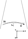 |
Fig. 1. Sketch of the magnetic reconnection outflow region with the TS. The upstream and downstream regions of the TS are located above and below the TS, respectively. The coordinate system employed in the paper is also drawn. |
The magnetic field, B, is put in the x − z plane and takes an angle, θ, to the x axis in the upstream region. All of the quantities with the subscript 1 or 2 denote those in the upstream and downstream regions, respectively. These Rankine–Hugoniot relationships were evaluated for the special case of a nearly perpendicular, fast-mode shock – θ → 90° – leading to

(see Eq. (A.9) in Mann 2018 for the jump in the magnetic field) and
(see Eq. (A.8) in Mann 2018 for the jump in the temperature). Here, X = ρ2/ρ1 denotes the jump in the mass density across the shock. The mass density, ρ, is related to the full particle number density, N, by  (mp, proton mass;
  , mean molecular weight; Priest 1982). The equation of state, p = NkBT (kB, Boltzmann’s constant), relates the pressure, p, to the full particle number density, N, and the temperature, T. Here, the Alfvén velocity and sound speed are given by vA1 = B1/(4πρ1)1/2 and
  (γ, ratio of the specific heats) in the upstream region, respectively. In the flare region, vA, 1 ≫ cs, 1 can be assumed, as is shown in Sect. 4. Then, according to the Rankine-Hugoniot relationships, the Alfvén-Mach number MA = vs/vA1 of the shock is related to the density jump, X, by
![$$ \begin{aligned} M_{\rm A} = \sqrt{X \cdot \frac{ [\gamma +X(2-\gamma )]}{[(\gamma +1)-X(\gamma -1)]}} \end{aligned} $$](/articles/aa/full_html/2024/06/aa49162-24/aa49162-24-eq6.gif)
(see Eq. (A.10) in Mann 2018) with the shock speed, vs.
The TS is a fast magnetosonic shock that is connected with positive jumps in the mass density, the magnetic field, and the temperature. Now, we look to the jump of the temperature at the TS (see Eq. (2)). Crucially, it depends on the ratio vA, 1/cs1. This ratio is ≫1 in flare regions, as is discussed in Sect. 4. Hence, the plasma is strongly heated from the temperature in the upstream region, T1, up to a temperature in the downstream region of the TS, T2, under special circumstances in flare regions. Thus, it could be that there are relativistic electrons in the tail of the electron distribution function (EDF) in the downstream region. Next, we calculated the part of electrons with energies beyond an energy, E*, in the downstream EDF.
To do that, we assumed a Maxwellian EDF in the downstream regions with temperature T2:
Microwave and hard X-ray observations during the flare on September 10, 2017 reveal that the EDF in the loop-top region consists of a thermal core and a broken power law in the energetic tail (see Fig. 3c in Chen et al. 2021 and the third paragraph of Sect. 3). Such an EDF is described by several parameters as the temperature of the thermal core as well as the break energy and the power law indices of the broken power law. In contrast to such an EDF, a Maxwellian one has only one parameter, namely the temperature. Unfortunately, the parameters of a broken power law cannot be determined by macroscopic relationships such as, for example, the equation of momentum. Since the Rankine–Hugoniot relationships result from the macroscopic MHD equations, these relations do not allow one to derive any information about the change in the parameters of the broken power law across the shock, such as the power law indices, for instance. For these reasons and for simplicity’s sake, we chose a Maxwellian EDF in the downstream region, since it has only the temperature, T, as the parameter and the Rankine–Hugoniot relationships provide information about the jump in the temperature across the shock.
In order to derive the differential electron number density, we followed the approach presented in the paper by Mann (2018). The kinetic energy, Ekin, of an electron with the momentum, p (p = ∥p∥), is given by  (me, electron mass). The constant, CM, can be fixed to
(see Eq. (3.14) in Mann 2018), with ϵ = Ekin/mec2 and ϵth = kBT2/mec2, if the EDF is normalized to unity. Then, the number density, Ne(ϵ*), of electrons with energies beyond E* is found to be

with ϵ* = E*/mec2 and Ne, 0 as the complete electron number density. Then, the differential electron number density defined by
results from Eq. (6) as
in the case of a Maxwellian EDF with temperature T2.
3. Solar flare on September 10, 2017
The solar event on September 10, 2017 was an X8.2 flare and the second-largest one in solar cycle 24. Since it appeared at the limb, it is an unique event through which to study the flare scenario in an excellent manner. It was described in detail from different points of view (Veronig et al. 2018; Warren et al. 2018; Gary et al. 2018; Longcope et al. 2019; Hayes et al. 2019; Morosan et al. 2019; Chen et al. 2020; Yu et al. 2020; French et al. 2020; Reeves et al. 2020; Fleishman et al. 2020, 2022). This event confirms well the standard (CSHKP) flare model. It showed an erupting flux rope with a CME and an underlying current sheet. The event was also acompanied by an SEP event (Guo et al. 2018) and a long-lasting (≈12 h) γ-ray emission with energies > 100 MeV (Omodei et al. 2018).
In this event, signatures of a long hot current sheet were observed behind the erupting flux rope (Seaton & Darnel 2018; Warren et al. 2018; Yan et al. 2018) in the flare region. This led to the formation of a large-scale reconnection current sheet (RCS). The mircrowave spectral imaging observations with the EOVSA instrument (Gary et al. 2018) reveals that relativistic electrons are present in the region between the erupting flux rope and the underlying flare loop arcade (Chen et al. 2020). Inspection of Fig. 2a in Chen et al. (2020) shows that the RCS extends in the height range of 20–70 Mm in projection above the limb. Chen et al. (2020) identified the RCS as a bright feature in the 193 Å band. It was observed by the “Atmospheric Imaging Assembly” (AIA, Lemen et al. 2012) instrument on board the “Solar Dynamics Observatory” (SDO, Pesnell et al. 2012). The 193 Å band is sensitive for hot plasmas with a temperature of about 18 MK. Figure 3a in Chen et al. (2020) reveals that the X and Y points are located at heights of ≈32 Mm and ≈20 Mm above the limb in projection, respectively. According to numerical simulations (Forbes 1986, 1988; Forbes & Malherbe 1986; Workman et al. 2011; Takasao et al. 2015; Takasao & Shibata 2016; Takahashi et al. 2017; Shen et al. 2018; Kong et al. 2019), the TS is predicted in the region between the Y point and the underlying flare loop arcade. Hence, the TS is expected in the height region of about 20 Mm in the event on September 10, 2017. There, an enhanced hard X-ray radiation is observed. The hard X-ray source observed by the RHESSI spacecraft (Lin et al. 2002) is located at the top of the flare loop arcade with a FWHM size of ≈20″ × 30″ (or 14.5 Mm × 21.8 Mm) (see Figs. 1a and 1d in Chen et al. 2021). There, the number density of electrons with energies beyond 300 keV is much greater, as is shown in Fig. 3e in Chen et al. (2020). That is an indication that the TS could be the source of these relativistic electrons, as was proposed by Tsuneta & Naito (1998).
The microwave data of the EOVSA instrument (Gary et al. 2018) and the hard X-ray data of the RHESSI instruments allow one to derive the EDF at the loop-top source of this event. Chen et al. (2021) did that for a broad energy range, 10 keV−1 MeV, during the early impulsive phase of the flare by means of the forward fitting method (Holman et al. 2003). The resulting EDF consists of a thermal core with a temperature of ≈25 MK, a broken power law in the energetic tail beyond ≈16 keV, and an electron power law index of ≈3.6. Beyond ≈160 keV, the power law breaks to a power law with an index of ≈8.5 (see Fig. 3c in Chen et al. 2021).
The upstream and downstream regions of the TS are located in the regions between the Y point and the TS and between the TS and the flare loop arcade, respectively. There, we find a temperature of T1 = 18 MK in the upstream region (see Fig. 2a in Chen et al. 2020 and also Warren et al. 2018) as well as an electron number density, Ne, 2 = 1010 cm−3, and magnetic field, B2 = 400 G (see Fig. 3b in Chen et al. 2020), in the downstream region as the plasma parameters at the TS. Furthermore, the number density of electrons with energies > 300 keV is found to be ≈1.6 × 104 cm−3 (because of log[Ne,>300 keV(cm−3)] = 4.2 in Fig. 3e in Chen et al. 2020) below the Y point.
4. Discussion
The aim of this section is to show that the heating of the plasma at the TS provides enough relativistic electrons in the downstream region of the TS by employing data from the solar event on September 10, 2017 (see Sect. 3).
As was mentioned in Sect. 3, the temperature T1 = 18 MK (corresponding to an energy of 1.55 keV) is found in the upstream region of the TS. It results in a sound speed of  km s−1 for γ = 5/3. Furthermore, a magnetic field strength of B2 = 400 G and an electron number density of Ne, 2 = 1010 cm−3 are adopted in the downstream region, leading to an Alfvén velocity of
  km s−1 for
  (Priest 1982)1 Thus, the ratio vA, 2/cs, 1 = 12.6 – the assumption that (vA, 2/cs, 1)2 ≫ 1 to derive Eq. (3) – is well justified.
Next, the ratio T2/T1 had to be calculated by means of Eq. (2). Inserting Eq. (3) for MA in Eq. (2) and taking into account vA, 1 = vA, 2/X1/2, one gets
The jump in the temperature, T2/T1, across the TS increases from one to infinity if X changes from one to four. It is calculated for several values of the density jump, X, varying in the range of 1.1–1.6 by means of Eq. (9) and vA, 2/cs, 1 = 12.6. The results are summarized in Table 1. Additionally, the electron number density, Ne, 1, the magnetic field, B1, and the Alfvén velocity, vA, 1, of the upstream region are also listed in Table 1.
Parameters of the TS according to the Rankine–Hugoniot relationships for density jumps, X, in the range of 1.1–1.6 for the plasma conditions measured during the solar event on September 10, 2017, i.e., the temperature, T1 = 18 MK, in the upstream region as well as the electron number density, Ne, 2 = 1010 cm−3, and the magnetic field, B2 = 400 G, in the downstream region.
The sixth column reveals that the plasma is strongly heated across the TS. The thermal energies in the downstream region, kBT2, are given in the sixth column of Table 1. They vary from 16.7 keV to 70.9 keV for a TS with Alfvén-Mach numbers, MA, in the range of 1.10–1.60, respectively.
Since the plasma is heated in the downstream region, a Maxwellian EDF was assumed there for simplicity’s sake (see also the discussion in Sect. 2). The number density of electrons with energies beyond 300 keV, Ne, 2 > 300 keV, was calculated with Eq. (6) for different values of the density jump, X, in the range of 1.1–1.6, as is presented in the seventh column in Table 1. We note that the EDF was treated in a fully relativistic manner in Sect. 2. The measurements with EOVSA (Gary et al. 2018) during the solar event on September 10, 2017 provide Ne, 2 > 300 keV = 1.58 × 104 cm−3 (see Sect. 3 and Fig. 3e in Chen et al. 2020) or Ne, 2 > 300 keV/Ne, 2 = 1.58 × 10⁻⁶ for Ne, 2 = 1010 cm−3. Inspecting Table 1, such a value of Ne, 2 > 300 keV/Ne, 2 is found for a TS with a density jump of 1.12 and an Alfvén-Mach number of 1.09. Thus, the TS with these special parameters is able to heat the downstream plasma from 1.55 keV up to 19.4 keV, and hence to explain the production of relativistic electrons during the solar event on September 10, 2017.
The TS considered is a low Alfvén-Mach number shock. Adopting the plasma parameters in the upstream region of the TS as derived here (see Table 1), the upstream flow has a velocity of vTS = 8342 km s−1. At the TS, which is a fast magnetosonic shock, the kinetic energy of the upstream flow is transformed into an increase in the temperature (heating) and the magnetic field in the downstream region (see Priest 1982). This flow carries a total energy density of2wtotal = wkin + wmag = 1.027 × 10⁴ erg cm−3, with a kinetic energy density of  erg cm−3 and a magnetic energy density of
  erg cm−3. Hence, an energy of ≈641 keV is available for each electron. This result demonstrates that the inflow in the upstream region contains enough energy to produce energetic electrons up to relativistic energies by means of heating at a low Alfvén-Mach number shock (such as MA = 1.09, for instance).
To illustrate this, Fig. 2 shows the differential electron number density of this special TS in the downstream (full line) and upstream regions (dashed line). It reveals that the electrons are strongly energized up to relativistic energies at the transition through the TS. There is a pronounced part of relativistic energies in the downstream region in the event under study. 58% of all electrons reach energies beyond 20 keV (see the eighth column in Table 1). This result agrees with the EOVSA observations (Fleishman et al. 2022) and confirms that the energetic electrons carry a substantial part of the energy released during flares (Lin & Hudson 1971, 1976; Emslie et al. 2004; Krucker et al. 2010; Krucker & Battaglia 2014).
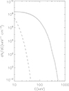 |
Fig. 2. Energy dependence of the differential electron number density, dNe/dE, for plasma with a thermal energy of 1.55 keV (ϵth, 1 = 0.0030 and Ne, 1 = 8.929 × 109 cm−3; dashed line) and 19.4 keV (ϵth, 2 = 0.0379 and Ne, 2 = 1010; full line) according to Eq. (8). |
Chen et al. (2021) derived electron energy spectra for the event on September 10, 2017 by means of a combined analysis of hard X-ray and microwave data measured by RHESSI (Lin et al. 2002) and EOVSA (Gary et al. 2018), respectively. Figure 3c in Chen et al. (2021) shows the differential electron number density (thick black curve) for the impulsive phase of this event. It consists of a thermal (i.e., Maxwellian) core and a broken power law in the energetic tail. Fig. 3c in Chen et al. (2021) and Fig. 2 of this paper are presented on the same scale. The comparison of these figures reveals that the differential electron number density resulting from the heating at the TS (see full line in Fig. 2) agrees roughly with the differential electron density obtained from the observations (thick black curve of Fig. 3c in Chen et al. 2021). We note that Chen et al. (2021) derived a broken power law for the differential electron number density, whereas the heating at the TS results in a Maxwellian EDF. (With respect to this subject, we refer to the discussion in Sect. 2).
Previously, Mann et al. (2006, 2009) and Warmuth et al. (2009) proposed the generation of energetic electrons at the TS by SDA. It is well known that SDA immediately produces a beam-like EDF (Mann 2018) in the upstream region of the shock. In contrast to these studies, here we demonstrate using the example of the September 10, 2017 flare that the heating of the plasma across the TS provides enough energetic electrons up to the relativistic energies needed for the microwave and hard X-ray emission. The resulting EDF is not beam-like as in the case of SDA but has a broad pronounced part at relativistic energies (see Fig. 2).
5. Summary and conclusions
There are signatures of a TS in the magnetic reconnection outflow region in solar radio (Aurass et al. 2002; Aurass & Mann 2004; Chen et al. 2015) and EUV (Polito et al. 2018; Cai et al. 2021) observations as well as numerical simulations (Forbes 1986, 1988; Forbes & Malherbe 1986; Workman et al. 2011; Takasao & Shibata 2016; Takahashi et al. 2017; Shen et al. 2018; Kong et al. 2019). Tsuneta & Naito (1998) proposed the TS as the source of energetic electrons responsible for the hard X-ray loop-top sources observed in solar flares.
The X8.2 solar flare on September 10, 2017 Chen et al. (2020) gives us a unique opportunity to study the generation of energetic electrons with observations from the EOVSA instrument Gary et al. (2018). This event clearly supports the standard (CSHKP) model of eruptive flares. Signatures of a current sheet were identified by Warren et al. (2018) and Chen et al. (2020). Relativistic electrons were produced in the vicinity of this current sheet. A value of 1.6 × 10⁴ electrons per cm3 with energies > 300 keV was derived from the EOVSA microwave images and spectra in the region between the lower end of the current sheet and the underlying loops; that is, the microwave emitting energetic electrons are strongly concentrated in the loop-top region. This finding can be explained by the presence of a TS in the region between the lower end of the current sheet and the underlying flare loops. The excellent EOVSA data of this event (Chen et al. 2020) allows one to determine the plasma parameters in the upstream and downstream regions of the TS. Adopting these parameters, we investigated the jump in the temperature across the shock by means of the Rankine–Hugoniot relationships (see Table 1). We show that a low Alfvén-Mach number TS with MA ≈ 1.09 is able to produce enough of the relativistic electrons needed to explain the microwave radiation measured by the EOVSA instrument in the September 10, 2017 flare. A substantial fraction – namely, 58% – of all electrons gain an energy beyond 20 keV.
In conclusion, the generation of relativistic electrons by heating the plasma at the TS is a possible mechanism of producing energetic electrons up to the relativistic energies needed for microwave and hard X-ray emission during large solar flares. The reason is that a large ratio between the Alfvén velocity and the sound speed upstream of the TS leads to a strong energizing of the downstream plasma.
In the coronal plasma, the full particle number N density is related to the electron number density Ne by N = 1.92Ne (Mann et al. 1999).
Acknowledgments
GM and FS express their thanks to the financial support by the Deutsches Zentrum für Luft- und Raumfahrt (DLR) under the grant 50 OT 2304. AMV aknowledges the Austrian Science Fund (FWF) under the grant 10.55776/14555.
References
- Aschwanden, M. J. 2005, Physics of the Solar Corona (Chichester: Praxis Publishing Ltd) [Google Scholar]
- Aurass, H., & Mann, G. 2004, ApJ, 615, 426 [Google Scholar]
- Aurass, H., Vršnak, B., & Mann, G. 2002, A&A, 384, 273 [NASA ADS] [CrossRef] [EDP Sciences] [Google Scholar]
- Cai, Q., Feng, H., Ye, J., & Shen, Ch. 2021, ApJ, 912, 79 [CrossRef] [Google Scholar]
- Carmichael, H. 1964, NASA Spec. Pub., 50, 451 [NASA ADS] [Google Scholar]
- Chen, B., Bastian, T. S., Shen, C., et al. 2015, Science, 350, 6265 [NASA ADS] [Google Scholar]
- Chen, B., Shen, C., Gary, D. E., et al. 2020, Nat. Astron., 4, 1140 [Google Scholar]
- Chen, B., Battaglia, M., Krucker, S., Reeves, K. K., & Glesener, L. 2021, ApJ, 908, 55 [NASA ADS] [CrossRef] [Google Scholar]
- Cheng, X., Li, Y., Wan, L. F., et al. 2018, ApJ, 866, 64 [Google Scholar]
- Emslie, A. G., Kucharek, H., Dennis, B. R., et al. 2004, J. Geophys. Res., 109, 10104 [NASA ADS] [Google Scholar]
- Fleishman, G. D., Gary, D. E., Kuroda, N., Yu, S., & Nita, G. M. 2020, Science, 367, 278 [NASA ADS] [CrossRef] [Google Scholar]
- Fleishman, G. D., Nita, G. M., Chen, B., Yu, S., & Gary, D. E. 2022, Nature, 606, 674 [NASA ADS] [CrossRef] [Google Scholar]
- Forbes, T. G. 1986, ApJ, 305, 553 [NASA ADS] [CrossRef] [Google Scholar]
- Forbes, T. G. 1988, Sol. Phys., 117, 97 [CrossRef] [Google Scholar]
- Forbes, T. G., & Malherbe, J. M. 1986, ApJ, 302, L67 [NASA ADS] [CrossRef] [Google Scholar]
- French, R. J., Matthews, S. A., van Driel-Gesztelyi, L., Long, D. M., & Judge, P. G. 2020, ApJ, 900, 192 [NASA ADS] [CrossRef] [Google Scholar]
- Gary, D. E., Chen, B., Dennis, B. R., et al. 2018, ApJ, 863, 83 [CrossRef] [Google Scholar]
- Guo, J., Dumbović, M., Wimmer-Schweingruber, R., et al. 2018, Space Weather, 16, 1156 [NASA ADS] [CrossRef] [Google Scholar]
- Hayes, L. A., Gallagher, P. T., Dennis, B. R., et al. 2019, ApJ, 875, 33 [Google Scholar]
- Heyvaerts, J. 1981, Solar Magnetohydrodynamica (London: Gordon and Breach) [Google Scholar]
- Hirayama, T. 1974, Sol. Phys., 34, 323 [Google Scholar]
- Holman, G. D., Sui, L., Schwartz, R. A., & Emslie, A. G. 2003, ApJ, 595, L97 [CrossRef] [Google Scholar]
- Klein, K.-L., & Trottet, G. 2001, Space Sci. Rev., 95, 215 [NASA ADS] [CrossRef] [Google Scholar]
- Kong, X., Guo, F., Shen, C., et al. 2019, ApJ, 887, L37 [NASA ADS] [CrossRef] [Google Scholar]
- Kopp, R., & Pneuman, G. W. 1976, Sol. Phys., 50, 85 [NASA ADS] [CrossRef] [Google Scholar]
- Krucker, S., & Battaglia, M. 2014, ApJ, 780, 107 [Google Scholar]
- Krucker, S., Hudson, H. S., Glesener, L., et al. 2010, ApJ, 714, 1108 [NASA ADS] [CrossRef] [Google Scholar]
- Lemen, J. R., Title, A. M., Akin, D. J., et al. 2012, Sol. Phys., 275, 17 [Google Scholar]
- Lin, R. P. 1974, Space Sci. Rev., 16, 189 [NASA ADS] [CrossRef] [Google Scholar]
- Lin, R. P., & Hudson, H. S. 1971, Sol. Phys., 17, 412 [NASA ADS] [CrossRef] [Google Scholar]
- Lin, R. P., & Hudson, H. S. 1976, Sol. Phys., 50, 153 [NASA ADS] [CrossRef] [Google Scholar]
- Lin, R. P., Dennis, B. R., Hurford, G. J., et al. 2002, Sol. Phys., 210, 3 [Google Scholar]
- Longcope, D., Unverferth, J., Klein, C., McCarthy, M., & Priest, E. 2019, ApJ, 868, 148 [Google Scholar]
- Mann, G. 2018, J. Plasma Phys., 81, 475810601P [Google Scholar]
- Mann, G., Jansen, F., MacDowall, R. J., Kaiser, M. L., & Stone, R. G. 1999, A&A, 348, 614 [NASA ADS] [Google Scholar]
- Mann, G., Aurass, H., & Warmuth, A. 2006, A&A, 454, 969 [NASA ADS] [CrossRef] [EDP Sciences] [Google Scholar]
- Mann, G., Warmuth, A., & Aurass, H. 2009, A&A, 528, A104 [Google Scholar]
- Mann, G., Melnik, V. N., Rucker, H. O., Konovalenko, A. A., & Brazhenko, A. I. 2018, A&A, 609, A41 [NASA ADS] [CrossRef] [EDP Sciences] [Google Scholar]
- Masuda, S., Kosugi, T., Hara, H., Tsuneta, S., & Ogawara, Y. 1994, Nature, 371, 495 [CrossRef] [Google Scholar]
- Morosan, D. E., Carley, E. P., Hayes, L. A., et al. 2019, Nat. Astron., 3, 452 [Google Scholar]
- Omodei, N., Pece-Rollins, M., Longo, F., Allafort, A., & Krucker, S. 2018, ApJ, 865, L7 [NASA ADS] [CrossRef] [Google Scholar]
- Pesnell, W. P., Thompson, B. J., & Chamberlein, P. C. 2012, Sol. Phys., 275, 3 [NASA ADS] [CrossRef] [Google Scholar]
- Polito, V., Galan, G., Reeves, K. K., & Musset, S. 2018, ApJ, 865, 161 [NASA ADS] [CrossRef] [Google Scholar]
- Priest, E. R. 1982, Solar Magnetohydrodynamics (Dordrecht: Kluwer Academic Publishers), 199 [Google Scholar]
- Reames, D. V., Barbier, L. M., & Ng, C. K. 1996, ApJ, 466, 473 [NASA ADS] [CrossRef] [Google Scholar]
- Reeves, K. K., Polito, V., Chen, B., et al. 2020, ApJ, 905, 165 [NASA ADS] [CrossRef] [Google Scholar]
- Seaton, D. B., & Darnel, J. M. 2018, ApJ, 852, L9 [NASA ADS] [CrossRef] [Google Scholar]
- Shen, C., Kong, X., Guo, F., Raymond, J. C., & Chen, B. 2018, ApJ, 869, 116 [NASA ADS] [CrossRef] [Google Scholar]
- Shibata, K., Mausuda, S., Shimojo, M., et al. 1995, ApJ, 451, L83 [NASA ADS] [CrossRef] [Google Scholar]
- Sturrock, P. A. 1966, Nature, 211, 695 [Google Scholar]
- Treumann, R., & Baumjohann, W. 1997, Advances in Space Plasma Physics (London: London Imperial College Press), 143 [CrossRef] [Google Scholar]
- Takahashi, T., Qui, J., & Shibata, K. 2017, ApJ, 848, 102 [NASA ADS] [CrossRef] [Google Scholar]
- Takasao, S., & Shibata, K. 2016, ApJ, 823, 150 [NASA ADS] [CrossRef] [Google Scholar]
- Takasao, S., Matsumoto, T., Nakamura, N., & Shibata, K. 2015, ApJ, 805, 135 [NASA ADS] [CrossRef] [Google Scholar]
- Tsuneta, S., & Naito, T. 1998, ApJ, 495, L67 [NASA ADS] [CrossRef] [Google Scholar]
- Veronig, A. M., Podladchikova, T., Dissauer, K., et al. 2018, ApJ, 868, 107 [NASA ADS] [CrossRef] [Google Scholar]
- Warmuth, A., Mann, G., & Aurass, H. 2007, Cent. Eur. Astrophys. Bull., 31, 135 [Google Scholar]
- Warmuth, A., Mann, G., & Aurass, H. 2009, A&A, 494, 677 [NASA ADS] [CrossRef] [EDP Sciences] [Google Scholar]
- Warren, H. P., Brocks, D. H., Ugarte-Urra, I., et al. 2018, ApJ, 854, 122 [NASA ADS] [CrossRef] [Google Scholar]
- Workman, J. C., Blackman, E. G., & Ren, C. 2011, Phys. Plasma, 18, 092902 [NASA ADS] [CrossRef] [Google Scholar]
- Yan, X. L., Yang, L. H., Xue, Z. K., et al. 2018, ApJ, 853, L18 [Google Scholar]
- Yu, S., Chen, B., Reeves, K. U., et al. 2020, ApJ, 900, 17 [NASA ADS] [CrossRef] [Google Scholar]
- Zharkova, V. V., Arzner, K., Benz, A. O., et al. 2011, Space Sci. Rev., 159, 357 [Google Scholar]
All Tables
Parameters of the TS according to the Rankine–Hugoniot relationships for density jumps, X, in the range of 1.1–1.6 for the plasma conditions measured during the solar event on September 10, 2017, i.e., the temperature, T1 = 18 MK, in the upstream region as well as the electron number density, Ne, 2 = 1010 cm−3, and the magnetic field, B2 = 400 G, in the downstream region.
All Figures
|
Fig. 1. Sketch of the magnetic reconnection outflow region with the TS. The upstream and downstream regions of the TS are located above and below the TS, respectively. The coordinate system employed in the paper is also drawn. |
| In the text | |
|
Fig. 2. Energy dependence of the differential electron number density, dNe/dE, for plasma with a thermal energy of 1.55 keV (ϵth, 1 = 0.0030 and Ne, 1 = 8.929 × 109 cm−3; dashed line) and 19.4 keV (ϵth, 2 = 0.0379 and Ne, 2 = 1010; full line) according to Eq. (8). |
| In the text | |
Current usage metrics show cumulative count of Article Views (full-text article views including HTML views, PDF and ePub downloads, according to the available data) and Abstracts Views on Vision4Press platform.
Data correspond to usage on the plateform after 2015. The current usage metrics is available 48-96 hours after online publication and is updated daily on week days.
Initial download of the metrics may take a while.