| Issue |
A&A
Volume 527, March 2011
|
|
|---|---|---|
| Article Number | A140 | |
| Number of page(s) | 22 | |
| Section | Planets and planetary systems | |
| DOI | https://doi.org/10.1051/0004-6361/201015861 | |
| Published online | 11 February 2011 | |
Mass constraints on substellar companion candidates from the re-reduced Hipparcos intermediate astrometric data: nine confirmed planets and two confirmed brown dwarfs⋆,⋆⋆
ZAH – Landessternwarte, Königstuhl 12, 69117
Heidelberg,
Germany
e-mail: sreffert@lsw.uni-heidelberg.de
Received:
4
October
2010
Accepted:
22
December
2010
Context. The recently completed re-reduction of the Hipparcos data by van Leeuwen (2007a, Astrophysics and Space Science Library, 350) makes it possible to search for the astrometric signatures of planets and brown dwarfs known from radial velocity surveys in the improved Hipparcos intermediate astrometric data.
Aims. Our aim is to put more significant constraints on the orbital parameters which cannot be derived from radial velocities alone, i.e. the inclination and the longitude of the ascending node, than was possible before. The determination of the inclination in particular allows to calculate an unambiguous companion mass, rather than the lower mass limit which can be obtained from radial velocity measurements.
Methods. We fitted the astrometric orbits of 310 substellar companions around 258 stars, which were all discovered via the radial velocity method, to the Hipparcos intermediate astrometric data provided by van Leeuwen.
Results. Even though the astrometric signatures of the companions cannot be detected in most cases, the Hipparcos data still provide lower limits on the inclination for all but 67 of the investigated companions, which translates into upper limits on the masses of the unseen companions. For nine companions the derived upper mass limit lies in the planetary and for 75 companions in the brown dwarf mass regime, proving the substellar nature of those objects. Two of those objects have minimum masses also in the brown dwarf regime and are thus proven to be brown dwarfs. The confirmed planets are the ones around Pollux (β Gem b), ϵ Eri b, ϵ Ret b, μ Ara b, υ And c and d, 47 UMa b, HD 10647 b and HD 147513 b. The confirmed brown dwarfs are HD 137510 b and HD 168443 c. In 20 cases, the astrometric signature of the substellar companion was detected in the Hipparcos data, resulting in reasonable constraints on inclination and ascending node. Of these 20 companions, three are confirmed as planets or lightweight brown dwarfs (HD 87833 b, ι Dra b, and γ Cep b), two as brown dwarfs (HD 106252 b and HD 168443 b), and four are low-mass stars (BD –04 782 b, HD 112758 b, ρ CrB b, and HD169822 b). Of the others, many are either brown dwarfs or very low mass stars. For ϵ Eri, we derive a solution which is very similar to the one obtained using Hubble Space Telescope data.
Key words: astrometry / binaries: spectroscopic / planetary systems / brown dwarfs
Table 1 and Appendix are only available in electronic form at http://www.aanda.org
© ESO, 2011
1. Introduction
Most of the around 400 planets and planet candidates known so far1 have been detected with the radial velocity method. As is very well known, only five of the seven orbital parameters which characterize a binary orbit can be derived from radial velocity observations (period, periastron time, eccentricity, longitude of periastron and either the mass function, the radial velocity semi-amplitude, the semi-major axis of the companion orbit or the semi-major axis of the primary orbit times the sine of the inclination). The remaining two orbital parameters, inclination and longitude of the ascending node2, are related to the orientation of the orbit in space and cannot be derived from radial velocities alone. Unfortunately, this means that the true companion mass is usually not known for planets detected via radial velocities; the only quantity which can be derived is a lower limit for the companion mass, which is the true companion mass times the sine of the inclination. Strictly speaking, all substellar companions detected via the radial velocity technique would thus have to be called planet or brown dwarf candidates since their true mass is not known.
In order to establish substellar companion masses, a complementary technique is required which is sensitive to the inclination. For companions with inclinations close to 90°, transit photometry can provide the inclination and thus, among other information, an accurate companion mass. For most systems however this is not the case, and astrometry is the method of choice. Astrometry provides both missing parameters, the inclination and the ascending node, so that the orbits are fully characterized. In principle, all orbital parameters can be derived from astrometric measurements, but since with current techniques the radial velocity parameters are usually more precise, another option is to derive only the two missing orbital parameters from the astrometry.
The astrometric signatures of planetary companions are rather small compared to the
astrometric accuracies which are currently achievable. The astrometric signature
αmax can be calculated if the radial velocity semi-amplitude
K1, the period P, the eccentricity
e, the inclination i and the parallax ϖ
are known (see e.g. Heintz 1978, or any other book on
double stars):  (1)αmax corresponds to
the semi-major axis of the true orbit of the photocenter around the center of mass. This is
however in general not the astrometric signature which is observable from Earth in the case
of eccentric orbits, due to projection effects. In the worst case, the semi-major axis of
the projected orbit corresponds to the semi-minor axis of the true orbit only, while the
semi-minor axis of the projected orbit could be identical to zero, so that no astrometric
signal can be observed along that direction. The astrometric signature α
which is actually observable from Earth can be calculated with the formulae for ellipse
projection given in Appendix A.
(1)αmax corresponds to
the semi-major axis of the true orbit of the photocenter around the center of mass. This is
however in general not the astrometric signature which is observable from Earth in the case
of eccentric orbits, due to projection effects. In the worst case, the semi-major axis of
the projected orbit corresponds to the semi-minor axis of the true orbit only, while the
semi-minor axis of the projected orbit could be identical to zero, so that no astrometric
signal can be observed along that direction. The astrometric signature α
which is actually observable from Earth can be calculated with the formulae for ellipse
projection given in Appendix A.
If the inclination is unknown, as is the case when the orbit is derived from radial
velocities alone, Eq. (1) provides a lower
limit for the astrometric signature by setting sini = 1 and multiplying
with 1 − e2 (converting the semi-major into the semi-minor
axis):  (2)We note that a more stringent lower limit on
the observable astrometric signature could be obtained if the longitude of the periastron is
taken into account; the above lower limit for the astrometric signature corresponds to the
case where the longitude of the periastron is ± 90°.
(2)We note that a more stringent lower limit on
the observable astrometric signature could be obtained if the longitude of the periastron is
taken into account; the above lower limit for the astrometric signature corresponds to the
case where the longitude of the periastron is ± 90°.
Instead of the semi-amplitude K1, one could also use the mass function or the semi-major axis of the primary orbit, multiplied by sini, as an alternative orbital element to express the unique relation between astrometric signature and various orbital elements.
Equation (1) shows that we can always derive an upper mass limit for the companion based on astrometry if the companion mass times the sine of the inclination, m2·sini, is known from radial velocities. The astrometry provides an upper limit on the astrometric signature of the companion, which translates into a lower limit on the inclination (Eq. (1)). In combination with the minimum companion mass m2·sini, the lower limit on the inclination translates into an upper limit of the companion mass m2.
For example, the astrometric signature of a companion with a mass of 1 MJup and a period of five years orbiting around a solar-mass star located at a distance of 10 pc amounts to 0.28 mas, not taking projection effects into account. Although this value is rather small, several astrometric detections of substellar companions have been reported in the past, mostly for systems with rather long periods and relatively massive companions around nearby stars, which all help to increase the astrometric signal.
Based on the Hipparcos data, 58 derived upper mass limits of 22 MJup for the substellar companion to 47 UMa and of 65 MJup for the companion to 70 Vir, with 90% confidence. This confirmed for the first time the substellar nature of these newly detected companions. For 51 Peg with its period of only a few days no useful upper mass limit could be established based on Hipparcos data.
Mazeh et al. (1999) and 87 followed that same approach to derive masses or upper mass limits for
the companions to υ And and HD 10697, respectively. For the outermost
companion in the υ And system, Mazeh et al. (1999) derived a mass of 10.1 MJup at a
confidence level of 68.3% and a mass of 10.1
MJup at a
confidence level of 68.3% and a mass of 10.1 MJup at a
confidence level of 95.4%. For the companion to HD 10697, 87 obtained a mass of 38 ± 13 MJup, which implies that
the companion is actually a brown dwarf and not a planet. These studies were extended to all
the 47 planetary and 14 brown dwarf companion candidates known at the time in 88. For 14 planetary companions, the derived upper mass
limits imply that the companions are of substellar nature, but for the others no useful
upper mass limits could be derived. Similarly, even for the brown dwarfs the
Hipparcos astrometry is in general not precise enough to derive tight
upper limits or to establish the astrometric orbit. However, for six of the 14 brown dwarf
candidates it turned out that the companion was stellar, and the astrometric orbit could be
derived. This confirms the results of Halbwachs et al. (2000), who examined the Hipparcos astrometry for eleven stars
harboring brown dwarf candidates. Seven of those brown dwarf secondaries turned out to be of
stellar mass, while only one of the studied companions is, with low confidence, a brown
dwarf. For the other three candidates, no useful constraints could be derived. In a previous
paper (Reffert & Quirrenbach 2006), we derived
masses of 37
MJup at a
confidence level of 95.4%. For the companion to HD 10697, 87 obtained a mass of 38 ± 13 MJup, which implies that
the companion is actually a brown dwarf and not a planet. These studies were extended to all
the 47 planetary and 14 brown dwarf companion candidates known at the time in 88. For 14 planetary companions, the derived upper mass
limits imply that the companions are of substellar nature, but for the others no useful
upper mass limits could be derived. Similarly, even for the brown dwarfs the
Hipparcos astrometry is in general not precise enough to derive tight
upper limits or to establish the astrometric orbit. However, for six of the 14 brown dwarf
candidates it turned out that the companion was stellar, and the astrometric orbit could be
derived. This confirms the results of Halbwachs et al. (2000), who examined the Hipparcos astrometry for eleven stars
harboring brown dwarf candidates. Seven of those brown dwarf secondaries turned out to be of
stellar mass, while only one of the studied companions is, with low confidence, a brown
dwarf. For the other three candidates, no useful constraints could be derived. In a previous
paper (Reffert & Quirrenbach 2006), we derived
masses of 37 MJup for the
outer companion in the HD 38529 system, and of 34 ± 12 MJup for
the outer companion in the HD 168443 system, based on Hipparcos astrometry.
This established the brown dwarf nature of both objects. Most recently, 71 have followed that same approach to derive masses for
the two brown dwarf candidates orbiting HD 131664 and HD 43848, respectively. With a mass of
MJup for the
outer companion in the HD 38529 system, and of 34 ± 12 MJup for
the outer companion in the HD 168443 system, based on Hipparcos astrometry.
This established the brown dwarf nature of both objects. Most recently, 71 have followed that same approach to derive masses for
the two brown dwarf candidates orbiting HD 131664 and HD 43848, respectively. With a mass of
 MJup, the
companion to HD 131664 is indeed a brown dwarf, while the companion to HD 43848 turned out
to be stellar with a mass of
MJup, the
companion to HD 131664 is indeed a brown dwarf, while the companion to HD 43848 turned out
to be stellar with a mass of  MJup.
MJup.
Using the fine guidance sensors (FGS) of the Hubble Space Telescope (HST), an astrometric precision somewhat better than in the original Hipparcos Catalogue can be achieved. Single measurement accuracies of around 1 mas and parallaxes as accurate as about 0.2 mas have been determined (Benedict et al. 2007, 2009) with HST; the most accurate parallaxes in the original Hipparcos Catalogue are around 0.4 mas (for a few bright stars). An upper mass limit of about 30 MJup, at a confidence level of 99.73%, was derived by 45 for the companion to 55 Cnc b, based on HST/FGS data. Benedict et al. (2002) reported the first astrometrically determined mass of an extrasolar planet. They determined the mass of the outermost planet orbiting GJ 876 as 1.89 ± 0.34 MJup, at 68.3% confidence, based also on HST/FGS data. For the companion to ϵ Eri, 6 obtained a mass of 1.55 ± 0.24 MJup, again at 68.3% confidence and based on HST/FGS data. For the planet candidate around HD 33636, 4 derived a mass of 0.14 ± 0.01 M⊙ with the same method, implying that the companion is a low-mass star and not a planet or a brown dwarf.
Most recently, two brown dwarfs were confirmed with HST astrometry: HD 136118 b has a mass
of 42 MJup (Martioli
et al. 2010), and HD 38529 c has a mass of
17.6
MJup (Martioli
et al. 2010), and HD 38529 c has a mass of
17.6 MJup (Benedict
et al. 2010). In the υ And system,
the inclinations of two companions could be measured, which not only allowed for the
determination of their masses (13.98
MJup (Benedict
et al. 2010). In the υ And system,
the inclinations of two companions could be measured, which not only allowed for the
determination of their masses (13.98 MJup for
υ And c and 10.25
MJup for
υ And c and 10.25 MJup for
υ And d, McArthur 2010), but also
the mutual inclination could be shown to be 29.9 ± 1°. This is the first such measurement
and shows the potential of astrometry for the measurement of the 3-dimensional orbit
geometry in multiple systems.
MJup for
υ And d, McArthur 2010), but also
the mutual inclination could be shown to be 29.9 ± 1°. This is the first such measurement
and shows the potential of astrometry for the measurement of the 3-dimensional orbit
geometry in multiple systems.
The median precision of positions and parallaxes in the original version of the Hipparcos Catalogue is just better than 1 mas, which is rather good, but still not good enough to detect those typical planetary companions which have been identified by radial-velocity surveys.
However, a new reduction of the raw Hipparcos data has been presented by van Leeuwen (2007a). Through an improved attitude modeling, systematic errors which dominated the error budget for the brighter stars in particular were much reduced, by up to a factor of four compared to the original version of the catalog. The formal error on the most precise parallaxes in the original version of the Hipparcos Catalogue is around 0.4 mas, and around 0.1 mas in the new reduction presented by van Leeuwen (2007a). The new reduction has been clearly shown to be superior to the old reduction of the data in van Leeuwen (2007b). The smaller formal errors, in particular for the bright stars, greatly improve the prospect of finding astrometric signatures of planets and brown dwarfs in the data.
In this paper we take a new look at the Hipparcos intermediate astrometric data, based on the new reduction of the Hipparcos raw data by van Leeuwen (2007a), for a large number of stars with planetary or brown dwarf candidates from radial velocity surveys. With the improved astrometric accuracy, it might be possible to detect a companion or place a tighter limit on its mass than was possible before.
The outline of this paper is as follows: in Sect. 2, we describe the various input data for our study, including the stellar sample with known planetary and brown dwarf companion candidates as well as the astrometric data from Hipparcos. In Sect. 3, we explain how we fitted astrometric orbits to the new Hipparcos intermediate astrometric data. Results are presented in Sect. 4 (upper mass limits for the companions to all examined stars) and in Sect. 5 (a few stars for which the astrometric orbit could be detected). We conclude the paper with notes on individual stars in Sect. 6 and a summary and discussion in Sect. 7. In the appendix, we show how to calculate the astrometric signature and orientation of the apparent orbit from the true orbit, taking projection effects into account.
2. Data
2.1. Stellar sample
In an effort to be as exhaustive as possible, we put together a sample of all known planetary and brown dwarf companions to Hipparcos stars detected via radial velocities. We started with the list of planetary companions compiled by 10. We added those stars with substellar companion candidates which were detected after 2006, as well as stars with brown dwarf companions which were not included in the list by Butler. We removed stars which were either not in the Hipparcos Catalogue or for which no orbital elements were available, and we updated the orbital elements for those stars for which new solutions were published in the meantime.
We calculated periastron times for a few stars for which those were not given in the original table, namely transiting planets with circular orbits3 (HD 189733) and planetary systems with significant interaction between the companions (HD 82943, HD 202206 and GJ 876). For the latter, only osculating elements can be given, and periastron times were calculated close to the epoch to which the elements referred. For all three stars this was about a decade later than the Hipparcos epoch of J1991.25, so that the orbital elements available might not be representative for the time at which the Hipparcos measurements occurred.
Furthermore, we assume that the longitude of periastron which is given for spectroscopically detected extrasolar planets is actually the one pertaining to the star, since this is the component observed (we verified this for a few examples). The longitude of periastron of the two components differ by 180°; the distinction is important for the combination with positional data.
Our final list comprises 258 stars with 310 substellar companions and is current as of April 2010. All stars which were examined are listed in Table 1, along with one or more references to the orbital elements.
2.2. Hipparcos intermediate astrometric data
The new reduction of the Hipparcos Catalogue by van Leeuwen does not only include a new estimate of the standard five astrometric parameters (mean positions, proper motions and parallax) for every star, but also the improved individual measurements, the so-called intermediate astrometric data.
In contrast to the original solution, the given abscissa data are not averaged over all observations within an orbit in the van Leeuwen version. Rather, one abscissa residual is given per field transit, which increases the average number of individual abscissae available for an object. The noise level of the new abscissae is, after averaging, up to a factor of four smaller than before. The errors of the averaged abscissae (per epoch accuracies) in the new version of the Hipparcos Catalogue range from better than 0.7 mas for a few really bright stars up to around 10 mas for the faintest stars; most stars have abscissa errors between 1.5 and 5 mas (van Leeuwen 2007b).
Everything else is very similar as before, although instead of the partial derivative of each abscissa residual with respect to the five standard astrometric parameters, the new version gives the instantaneous scan orientation and the parallax factor instead. But this is just a different parameterization of the same information; all relevant quantities can be derived from that, as explained in van Leeuwen (2007a).
3. Orbit fitting
3.1. Method
We have fitted astrometric orbits to the new Hipparcos abscissa residuals for all stars listed in Table 1, simultaneously with corrections to the five standard astrometric parameters, via a standard least squares minimization technique. The only two orbital parameters fitted for were the inclination and the ascending node; all other five orbital parameters (period, periastron time, eccentricity, longitude of periastron and mass function) were kept fixed at the literature values found via fits to the radial velocity data of each star.
If the star had an orbital solution in the Hipparcos Catalogue with a period of the same order of magnitude as the spectroscopic one, we removed the astrometric signature of the orbit from the abscissa data using the astrometric orbital elements, and then fitted for the full orbit again using spectroscopic values as input. In other words, we did not fit for corrections to the orbit as applied in the Hipparcos Catalogue, but for the full orbit from scratch (this step is only necessary for the abscissa data provided by van Leeuwen 2007a, since in the original Hipparcos Catalogue the abscissae always corresponded to a single star solution, even if an orbit was provided). This applies to three stars in our sample: HD 110833 (HIP 62145), ρ CrB (HIP 78459), and HD 217580 (HIP 113718). Likewise, we removed the acceleration terms from the Hipparcos abscissa values if the solution was a 7 or 9 parameter solution before fitting for the astrometric orbit. This applies to the following five stars: HD 43848 (HIP 29804), 55 Cnc (HIP 43587), HD 81040 (HIP 46076), γ1 Leo A (HIP 50583), and HD 195019 (HIP 100970). Please also note that the version of the van Leeuwen catalog which is available in VizieR4 is different from the one provided together with the book from van Leeuwen (2007a). E.g., 55 Cnc (HIP 45387) has a 7 parameter acceleration solution in the book version, but a stochastic solution in the online version. Since the abscissae are only available based on the book version, this is what we used here.
For stars with more than one substellar companion candidate, we did not fit for these multiple companions simultaneously, but individually. This should be a reasonable approach, since in the vast majority of the cases only one of the companions will dominate the astrometric signal of the system. This is especially true for systems detected via radial velocities, since for those all companions tend to have similar radial velocity signals (i.e. the more massive companions will be located further out). The astrometry would then be dominated by that massive outer companion, whereas less massive inner companions have a much smaller astrometric signal not detectable in the Hipparcos data.
We explicitly used all five spectroscopic orbital parameters in the fitting process and kept them fixed. The radial velocity signal is in all the cases much more significant than the astrometric signal, so that orbital parameters derived from the radial velocities should also be more precise and accurate than those derived from the astrometry. Other authors have chosen to disregard some of the spectroscopic orbital parameters, e.g. the radial velocity semi-amplitude (Mazeh et al. 1999) or the longitude of the periastron (Pourbaix & Jorissen 2000) and then later compared the astrometrically derived value to the original, spectroscopic one, as a consistency check. However, we prefer not to disregard any spectroscopic information in our astrometric fits, since this would likely compromise the accuracy of the orbital parameters which we are most interested in and not obtainable otherwise, the inclination and the ascending node.
Likewise, we did not take the approach of fitting for the semi-major axis of the astrometric orbit and only later linking this to the spectroscopic values via the parallax, but applied all those constraints simultaneously and implicitly in the fitting process, which is a more direct approach and should yield the highest accuracy in the inclination and ascending node. We note that the criterion by Pourbaix & Jorissen (2000) which is often used to link spectroscopic and astrometric quantities is not exactly correct, as no allowance is made for projection effects. As detailed in the appendix, the semi-major axis of the apparent orbit is possibly smaller than the semi-major axis of the true orbit, especially for eccentric orbits with small inclinations.
Also, we did not compare the χ2 values of the standard solution (five parameters) and the one including the astrometric orbit (two additional orbital parameters) in an F test, as was done by Pourbaix & Jorissen (2000) to decide whether the astrometric orbit was detected in the Hipparcos data. The reason is that we do not want to evaluate whether the standard model or the orbital model is the better one since we assume that the existence of a companion has been established already by the radial velocity data. The question we would like to ask here is how well the astrometric orbit can be constrained with the Hipparcos abscissa data, and the most suitable criterion for this kind of question is the joint confidence region allowed for the two orbital parameters. A small confidence region, compared to the total allowed parameter range, indicates a detection of the orbit, whereas a large confidence region would indicate no real detection. In order to be conservative, we mostly use 3σ confidence regions, corresponding to a probability of 99.73% that the true value falls within this parameter interval.
In principle it would also be possible to fit for all orbital elements simultaneously using radial velocities as well as astrometry. 82 have developed an efficient algorithm which can fit several orbital companions to astrometric and radial velocity data jointly. Inclination and ascending node will always be derived from the astrometric data alone, since radial velocities are not sensitive to those parameters. The advantage of jointly fitting both kinds of data are better constraints on the five spectroscopic orbital parameters which now come from the two different data sets, as well as explicit covariances between all orbital parameters. However, since in virtually all the cases investigated here the companion signature is much more significantly detected in radial velocities than in astrometry (if at all), the weighting of the astrometric data in the combined fit would be much lower than that of the radial velocity data, and in the end the astrometry would not influence the values of the spectroscopic parameters. Therefore no attempt has been made here to combine precise radial velocities with Hipparcos astrometry. This situation should change once more accurate astrometry becomes available.
3.2. ϵ Eri
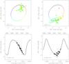 |
Fig. 1 Illustration of abscissa residuals from Hipparcos along with the astrometric orbit as fitted for ϵ Eri. The two panels in the top row show the abscissa residuals (colored dots) with respect to the standard astrometric model without orbiting companion (upper left) and with respect to a model (solid line) which includes the companion (upper right). The colored lines indicate the direction which was not measured and along which the dots are allowed to slide in the adjustment process; the actual abscissa measurement is perpendicular to that line. Color indicates orbital phase. The two panels in the bottom row show only one dimension each as a function of time. The solid line is the orbital model as in the upper panels, while the small grey dots are the individual abscissa residuals. The big black dots are averages of abscissa residuals taken very closely in time. The information about the orientation of the abscissa residuals is missing in the panels in the bottom row. |
An example for such an orbital fit is given in Fig. 1 for the case of ϵ Eri. The panels in the top row illustrate the 1-dimensional Hipparcos abscissa residuals (colored dots) in a 2-dimensional plot of the sky. The lines running through the colored dots indicate the direction which was not measured; the dots (measurements) are thus allowed to slide on that line. The actual measurement is perpendicular to the indicated line. The upper left panel shows the abscissa residuals with respect to the standard solution as given in the catalog, i.e. after fitting for the five standard astrometric parameters, while the panel on the upper right shows the abscissa residuals for the case where the orbiting companion has been taken into account. Thus, in the left panel the abscissa residuals are referred to the mean position of the star at (0, 0) in that diagram, while in the right panel the abscissa residuals refer to the corresponding points on the orbit which are indicated by small black dots. The solid line illustrates the astrometric orbit of the primary star as seen on the sky. The color indicates orbital phase; an abscissa residual of a given color refers to the point on the orbit with the same color. The time when a measurement was taken is an additional constraint in the fit, and the color coding is an attempt to visualize that additional constraint.
Alternatively, the two panels in the bottom row each show one dimension only as a function of time. The solid lines indicate the same orbit as in the panels in the top row. The smaller grey points indicate the individual abscissa residuals (for the case where the orbital model has been taken into account as in the upper right panel), while the bigger black dots show the mean of all abscissa residuals taken very closely together in time. This is for illustration purposes only; the fit was done using the individual, not the averaged abscissa residuals. When looking at the two panels in the bottom row please note that again not all constraints could be visualized at the same time; in these illustrations the information about the orientation of the abscissae is lost. The measurements as indicated in right ascension and declination are not static; due to the one-dimensional nature of the abscissa residuals the values plotted in the lower panels can change in the adjustment process.
One important complication which affects some of our orbital fits is immediately apparent: the Hipparcos measurements do not cover the full orbital phase range, but less than half of that for the 6.9 year period of ϵ Eri b. We will come back to that point when we discuss the ϵ Eri system in more detail in Sect. 6.
3.3. Verification
For verification purposes, we attempted to reproduce the inclinations and ascending nodes of spectroscopic binaries included in the Hipparcos Catalogue. There are 235 spectroscopic binaries for which an orbit is listed in the original Hipparcos Catalogue, and for 194 of those, the inclination and ascending node are actually obtained from a fit to the Hipparcos data (and not taken from some other reference). For those 194 stars we tried to reproduce the fitted inclinations and ascending nodes, using all other orbital elements as fixed input values (even if they were fitted for in Hipparcos), so that our approach resembles most closely the one which we are following with substellar companions detected with the radial velocity method. We used the original version of the Hipparcos Catalogue from 1997, because here the intermediate astrometric data correspond to the single star solution and because the orbital parameters are available electronically, which both helps in the fitting process.
We derived inclinations and ascending nodes with errors for all 194 systems and compared these values to the ones listed in the original Hipparcos Catalogue. In 78% of the cases, the two solutions agreed to within 0.3σ, and in 97% of the cases to within 1σ (although we note that the errors on the two angles can sometimes become rather large). Still, we consider this a very satisfactory result, and are thus confident that our method works correctly.
4. Upper mass limits for planets and brown dwarfs
While radial velocities provide m2 sini (where m2 is the companion mass and i is the inclination), a lower limit for the companion mass, astrometry can provide an upper mass limit for the companion. This is true even for stars where the astrometric signal of the companion is too small to be detectable, since inclinations approaching 0° or 180° (face-on orbits) would yield companions which are so massive at some point that they would show up in the astrometry. As the inclination of the orbit approaches a face-on configuration, there is always a limit at which the inclination is not compatible any more with the radial velocities and the astrometry. This means that even for companions which are not detected in the astrometry, there is usually still a (possibly weak) constraint on the inclination and thus on the mass of the companion.
In order to derive upper mass limits, we fitted astrometric orbits to the Hipparcos data for all stars on our list. The results are given in Table 1. The first two columns give the usual designation and the Hipparcos number, respectively. The following column indicates if more information on a particular star can be found in Sect. 6. The reference column gives a numerical code to the reference from which the spectroscopic orbital elements were taken; the code is explained at the end of the table. The period column gives the period in days according to the reference in the previous column; it is always derived from radial velocities. The following column gives the minimum mass m2 sini which corresponds to the orbital elements from the given reference; the star mass used in the conversion is also taken from the same reference. The last four columns give the result of our astrometric orbit fitting. The first three of those give the minimum and the maximum inclination corresponding to the 3σ confidence interval, imin and imax, and the resulting 3σ upper mass limit for the companion. In a few cases, an inclination of 90° could be excluded in the fitting. If this is the case, a new, more stringent lower mass limit could be derived, too, which is denoted as m2,min and given in the last column, if applicable. In some cases, especially when an inclination of 90° is not part of the inclination confidence region, there are two minima in the χ2 map, and the confidence region for the second minimum is given in a second line for that star. The table is sorted according to Hipparcos number (or right ascension, respectively).
For nine companions, the derived upper mass limit lies in the planetary mass regime, and thus unambiguously proves for the first time for most of them that these companions are really of planetary mass and not just planet candidates. The confirmed planets are β Gem b (Pollux b), ϵ Eri b, ϵ Ret b, μ Ara b, υ And c and d, 47 UMa b, HD 10647 b, and HD 147513 b. For ϵ Eri b and υ And c and d, the planetary nature was demonstrated already by HST astrometry, and for υ And d also by Hipparcos astrometry; see Sects. 6.1 and 6.2. For 47 UMa b, an upper mass limit in the brown dwarf regime at 90% confidence was obtained before, based on the original Hipparcos data, but the planetary nature could not be demonstrated unequivocally; see Sect. 6.3 for more details.
For a further 75 companions the derived upper mass limit lies in the brown dwarf mass regime and thus confirms at least the substellar nature of these companions. Two of those (HD 137510 b and HD 168443 c) have minimum masses also in the brown dwarf mass regime. These companions are established brown dwarfs now instead of just brown dwarf candidates. HD 168443 c was already confirmed to be a brown dwarf based on the original Hipparcos astrometry; see Sect. 6.6.
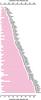 |
Fig. 2 Illustration of the allowed 3σ range of the companion mass for all stars from Table 1 for which the derived upper mass limit from Hipparcos corresponds to less than 85 MJup, i.e. for all 84 stars for which the substellar nature could be confirmed by Hipparcos. The lower mass limit usually corresponds to the lower mass limit m2 sini from the radial velocity fit, except for the few cases where the astrometry yields a tighter lower mass limit by excluding the inclination of 90° from the 3σ confidence region (HD 87883 b, HD 114783 b and γ Cep b). The upper mass limit always comes from the Hipparcos astrometry, according to Table 1. |
Figure 2 illustrates the results for those 84 companions from Table1 for which the substellar nature could be established. It can be seen that for many companions the allowed mass range between the lower mass limit from radial velocities and the upper mass limit from astrometry is still rather large. However, for a few of the companions this range is reasonably small (see e.g. ϵ Eri b, υ And d or ι Dra b), and one might even speak of a determination of the real companion mass rather than just placing a lower and upper limit on the mass, although there is a continuous transition between the two. In Sect. 5 we will take a closer look at those systems for which one might actually speak of a detection of the astrometric orbit, rather than just a constraint on the inclination and thus the mass.
4.1. Limitations
For some stars the formally derived 3σ upper mass limit of the companion is larger than 5 M⊙, which is not useful anymore. In fact, for astrometric upper mass limits larger than about 0.1–0.5 M⊙ there might be more useful upper mass limits based on photometry and/or spectroscopy. A stellar companion that massive would show up eventually in such data (see e.g. Kürster et al. 2008). It has not been attempted to derive those other upper mass limits here; the values given correspond to the limits set by astrometry, and only under the assumption that the companion does not contribute a significant fraction to the total flux in the Hipparcos passband. If the companion was bright enough to affect the photocenter of the system, our method would fail since we assume that the photocenter is identical to the primary component in the system, which we assume to be the Hipparcos star. If both components contribute significantly to the total flux, the observed orbit of the photocenter around the center of mass of the system depends on the difference between flux ratio and mass ratio of the two components. In order to model such a system, one would need to make additional assumptions about the components, which is beyond the scope of this paper.
Similarly, there are a number of stars for which the 3σ confidence interval in inclination extends from 0.1 to 179.9°. This is often the case for components with very small minimum masses and/or very small periods derived from Doppler spectroscopy, for which the astrometric signal is very small even for small inclinations. For those systems the derivation of the confidence interval in inclination is sometimes complicated by the fact that the fitting process does not converge for all possible inclinations, as well as by the limited resolution of our χ2 map in the interval between 0 and 0.1° or 179.9° and 180°, respectively. Of course it would be possible to increase the resolution for those inclination intervals (we already used higher resolution for the intervals from 0 to 1° and from 179° to 180° than for the rest of the inclination range), but the results would not be very meaningful since the method is just not suited very well for companions with extremely small astrometric signatures. As a consequence, the derived upper mass limits for those companions are not as accurate as those which correspond to inclinations which are not as close to 0 or 180°.
For 67 companions no upper mass limit could be derived at all from the Hipparcos astrometry. The reason is either that the astrometric fits did not converge (in 5000 iterations, which we set as a limit) over large parts of the inclination and ascending node parameter space, or that the 3σ confidence limits in inclination are very close to 0°or 180°, respectively, as mentioned above. In either case no meaningful confidence limits in inclination or upper mass limits could be derived. For those stars we list the whole inclination interval from 0° to 180° as 3σ confidence limits, and the column giving the 3σ upper mass limit is left empty in Table 1. 54 of the 67 companions without upper mass limits have periods smaller than 20 days, and 64 companions have periods smaller than 50 days and thus very small expected astrometric signatures.
5. Astrometric orbits
Best fit inclinations, ascending nodes and companion masses for stars where the astrometric orbit could be detected.
 |
Fig. 3 Illustration of the χ2 maps for those 20 stars for which the astrometric orbit could be detected in the Hipparcos data, as a function of inclination and ascending node. The contours show the 1σ, 2σ and 3σ confidence regions in both parameters jointly. Please note that for ρ CrB b the allowed range in inclination is so small that it is barely visible in this representation; the corresponding data can be found in Table 2. |
For a few of the stars in Table 1, not only upper mass limits could be derived, but also the astrometric orbit could be further constrained or fully determined. While for most companions a limit on the inclination could be derived (even if the lower limit is small), this is not necessarily true for the ascending node, the only other orbital element which is not determined by the radial velocity fit. This is due to the fact that an inclination approaching 0 degree will increase the size of the orbit, until eventually the orbit would not be compatible any more with the small scatter of the Hipparcos measurements. The ascending node however describes the orientation of the orbit in space. Thus usually no or very weak constraints can be placed on the ascending node if the orbit is not really detected. However, for 20 systems of Table 1 at least a weak constraint on the ascending node could be derived, indicating a (possibly weak) detection of the astrometric orbit. In contrast to Sect. 4, we now use the confidence levels for two parameters (inclination and ascending node) simultaneously, since we are now interested in the orbit, i.e. we want to derive constraints on both orbital parameters at the same time. Again, we used the contours pertaining to a probability of 99.73% (3σ). This will always result in a less tight constraint on the inclination than given in Table 1.
Those 20 systems with detected astrometric orbits are shown in Fig. 3 and listed in Table 2. The table gives the best-fit inclinations and ascending nodes, along with the 3σ confidence limits. Note that the 3σ confidence limits (denoted as imin, imax and Ωmin, Ωmax, respectively) are now confidence regions in two parameters, inclination and ascending node, as opposed to Table 1, where confidence limits in only one parameter (the inclination) were considered; the corresponding confidence regions in Table 2 are therefore slightly larger than those in Table 1. Please also note that for some stars, two minima are visible in the χ2 maps, often (but not always) with comparable local minimum χ2 values. Those solutions correspond to orbits of about the same size (similar inclinations), but with ascending nodes which differ by about 180°, so that the orbit has the opposite orientation. For those stars affected, we give in Table 2 the values pertinent to the second minimum in a second line for that star. For stars for which the confidence regions wrap around the 360° limit in the ascending node, continuing at 0°, we list the higher value as Ωmin and the lower one as Ωmax in order to indicate the correct orientation of the confidence region. The following three columns give the reduced χ2 values, the number nobs of individual 1-dim Hipparcos measurements (abscissae, or field transits) available for that star, and, for reference, the astrometric signature α for the fit.
Corrections (first rows) and final resulting values (second rows) of the five standard astrometric parameters (mean positions, parallax, proper motions) for the case where the astrometric modeling of the observations includes the effect of an orbiting companion.
The last four columns of Table 2 give the resulting masses for the astrometric solution. The minimum mass m2sini derived from the radial velocities is listed in the first of the four mass columns. This is also the minimum mass for any of the astrometric solutions, so it is given here for reference. It would correspond to an inclination of 90°. The next mass column labeled m2 gives the mass which corresponds to the best fit inclination. There is only one best fit mass for each system, so the second line is empty even if there are two minima. The next to last column, labeled m2,min, gives the lower limit for the 3σ confidence region in mass. If the inclination value of 90° is part of the 3σ confidence region (see also Fig. 3 or the columns imin and imax), then this value corresponds exactly to the minimum secondary mass derived from radial velocities. In order to indicate that this is the case, no mass is given here if appropriate. It can be seen that for twelve systems an inclination of 90° can be excluded with 99.73% confidence; for all others, the minimum secondary mass derived from radial velocities, m2sini, is within the 3σ mass confidence region and thus also the lower limit for the confidence region of the mass. Finally, the last column, labeled m2,max, gives the upper limit corresponding to the 3σ confidence region in mass.
Some orbits are rather well determined, even if using the conservative 99.73% confidence regions. The inclinations of BD –04 782 b, ρ CrB b and HD 169822 b could be determined to better than 5°, while the inclinations of HD 110833 b and HD 112758 b could be determined to better than 10°. For those systems, the ascending node is also rather well constrained. HD 168443 b could be confirmed as brown dwarf, even if taking the conservative 3σ confidence levels into account. ι Dra b is most likely a high-mass planet, while HD 106252 b and γ Cep b are most likely brown dwarfs. The companions for which the inclination could be determined to better than 5° are all low-mass stars.
Altogether, using the best fit masses, we find two planets (HD 87883 b and ι Dra b), eight brown dwarfs and ten stars among our 20 systems with astrometric orbits. Note that this is by no means representative for our whole sample listed in Table 1, since it is much more likely to find the astrometric signature of a star or a brown dwarf than the tiny signature of a planet in the Hipparcos data.
For completeness, we also list the corrections to the five standard astrometric parameters (mean positions at the Hipparcos epoch of J1991.25, parallax and proper motions) in the new Hipparcos Catalogue and the new resulting values for these in Table 3. These astrometric parameters were fitted simultaneously with the orbital parameters, and the changes are a direct consequence of the new fitting model which now includes the astrometric orbit. As usual, α ⋆ denotes a value where the cosδ has been factored in already. Note that the positional corrections are given in milli-arcseconds, whereas the coordinates themselves are given in radians, just like in the Hipparcos Catalogue by van Leeuwen (2007a). The corrections to the astrometric parameters are usually rather small, typically of the order or smaller than 1 mas or 1 mas yr-1, respectively.
6. Notes on individual stars
6.1. ϵ Eri (HIP 16537)
The presence of a planet orbiting ϵ Eri (HIP 16537, V = 3.7 mag) had long been suspected (Walker et al. 1995). In 2000, 27 finally announced the secure detection of ϵ Eri b, combining a variety of radial velocity data sets taken by different groups. It orbits its star in about 6.9 years, and has a minimum mass of msini = 0.86 MJup. Because of its small distance from the Sun (3.2 pc) the expected minimum astrometric signature amounts to 1.9 mas.
Using HST data in combination with data from the Multichannel Astrometric Photometer
(MAP) as well as radial velocities, 6 fit for the
astrometric orbit of ϵ Eri due to ϵ Eri b. They derive
an inclination of  and an ascending node of 74° ± 7°, yielding a mass for the companion of 1.55 ±
0.24 MJup.
and an ascending node of 74° ± 7°, yielding a mass for the companion of 1.55 ±
0.24 MJup.
This is in excellent agreement with the astrometric fit to the Hipparcos
data derived in this paper. Our best fit values are an inclination of 23° and an
ascending node of 282°, with 1σ errors of the order of 20° and a lower
limit for the inclination of 15° (1σ) and
 (3σ), respectively. We obtain a companion mass of
2.4 ± 1.1 MJup, slightly larger than the HST value. A second
minimum is found at an inclination of 158° and an ascending node of 53°, which is very
similar to the original orbit except that ascending and descending nodes are exchanged. We
do not consider the orbit detected in the Hipparcos data according to our
criterion chosen in Sect. 5, because the
3σ confidence region in inclination and ascending node jointly
encompasses the whole parameter range for the ascending node, and rather count
ϵ Eri among the stars with derived upper mass limits, but not with
detected orbital signatures.
(3σ), respectively. We obtain a companion mass of
2.4 ± 1.1 MJup, slightly larger than the HST value. A second
minimum is found at an inclination of 158° and an ascending node of 53°, which is very
similar to the original orbit except that ascending and descending nodes are exchanged. We
do not consider the orbit detected in the Hipparcos data according to our
criterion chosen in Sect. 5, because the
3σ confidence region in inclination and ascending node jointly
encompasses the whole parameter range for the ascending node, and rather count
ϵ Eri among the stars with derived upper mass limits, but not with
detected orbital signatures.
We have used the robust radial velocity fit from 27 as an input for our astrometric fit to the Hipparcos intermediate astrometric data. Formally the fit from 6 would have been the most precise one, but we preferred input parameters that came from a spectroscopic fit only instead of one which already was based on combined spectroscopy and HST astrometry. The slight differences which we find in companion masses are thus partly due to the use of different input data.
As mentioned already the phase coverage of the astrometric data is not complete. This applies to both the HST/FGS as well as the Hipparcos data; the HST/FGS data cover 2.9 years, while the Hipparcos data cover 2.5 years. This is to be compared with the orbital period of 6.9 years. Unfortunately, neither of the two astrometric data sets covers the phase of the orbit where the motion in right ascension is reversed, which would be very helpful to distinguish between orbital curvature and linear proper motion.
It is not straightforward to combine the Hipparcos data with the HST/FGS data from 6, since the reference points for the astrometry are different. In modeling the Hipparcos data, we have to simultaneously fit for orbital as well as astrometric parameters (mean absolute positions at the Hipparcos epoch of J1991.25, absolute proper motions and absolute parallax). In contrast to that, the HST/FGS astrometry is relative to a frame of standard stars, although the relative parallax has been converted into an absolute one by determining the parallaxes of the reference frame stars. In addition, the approach followed by 6 was to derive proper motions and parallaxes from measurements over a much larger time interval than their HST/FGS observations by including observations from the Multichannel Astrometric Photometer (MAP). If the Hipparcos and the HST/FGS data were to be combined, one would have to homogenize the astrometric parameters (positions, proper motions, parallaxes) and fit for additional zero-point offsets between the two datasets. However, since the zero-point of the HST/FGS proper motions is unknown, it is not possible to combine the two astrometric datasets in a rigorous way.
6.2. υ And (HIP 7513)
We derive rather tight constraints on the masses of the two outermost companions in the three planet system: an upper mass limit of 8.3 MJup (99.73% confidence) for υ And d, and an upper mass limit of 14.2 MJup for υ And c; the minimum masses determined from radial velocities are 4.13 MJup (υ And d) and 1.92 MJup (υ And c), respectively. Our newly derived upper mass limits place a much tighter constraint on the planet masses than was done before by Mazeh et al. (1999), who derived an upper mass limit of 19.6 MJup at 95.4% confidence for υ And d, using the original version of the Hipparcos Catalogue.
Most recently, rather accurate masses for those two companions in the
υ And system were measured from HST astrometry (McArthur et al. 2010): υ And d has a mass of
 MJup, and
υ And c has a mass of
MJup, and
υ And c has a mass of  MJup. The
corresponding best-fit inclinations are rather small
(
MJup. The
corresponding best-fit inclinations are rather small
( for υ And d and
  for υ And c). These results agree well with each other, although our
upper mass limits are both smaller than the measured HST masses.
for υ And c). These results agree well with each other, although our
upper mass limits are both smaller than the measured HST masses.
Since υ And is rather bright (V = 4.1 mag), the Hipparcos abscissae are not photon-noise dominated as for other stars, but are of comparable accuracy as the HST data. The single measurement precision is about 1 mas for both HST and Hipparcos. Hipparcos took data at 28 different epochs, covering 3.2 years, while the HST data refer to 13 different epochs, covering approximately 5 years. The precision per epoch is higher for HST, since more single measurements are averaged. Resulting parallaxes are rather precise for both HST and Hipparcos, with formal errors of 0.10 mas for the HST parallax and 0.19 mas for the Hipparcos parallax, respectively.
One should note further that our approach of fitting one companion candidate at a time to the astrometric data is not ideal in the υ And system, where the two outermost companions both contribute to the observed astrometric signal. However, it is unlikely that a combined fit of the two companions would lead to considerably higher upper mass limits; in general one would expect smaller astrometric signatures and thus smaller masses in a combined fit of the two companions as compared to a fit of both components separately. Thus our upper mass limits should hold even in the υ And system, although they might be too conservative.
6.3. 47 UMa (HIP 53721) and 70 Vir (HIP 65721)
For the companion to 47 UMa, an upper mass limit of between 7 (best fit) and 22 MJup (90% confidence level) was derived by 58, using the same method as we employ here, but with the original version of the Hipparcos Catalogue (ESA 1997). The minimum companion mass from the RV solution is 2.45 MJup. We derive a tighter constraint on the mass, with an upper mass limit of 9.1 MJup at 99.73% confidence, which demonstrates that the companion is a planet. The best fit value for the mass is 3.0 MJup, and the 1σ upper mass limit is 4.9 MJup.
An upper mass limit of 38–65 MJup was derived for the companion to 70 Vir by 58, where 38 MJup corresponds to the best fit, while 65 MJup corresponds to a confidence level of 90%. We derive an upper mass limit of 45.5 MJup, corresponding to a rather conservative confidence level of 99.73%. Our 1σ upper mass limit would be 26.8 MJup, smaller than the best fit value of 58.
For 51 Peg (HIP 113357), neither 58 nor we could derive a very meaningful result; the upper mass limit derived is around 0.5 M⊙ in both investigations.
Overall, our results are thus fully consistent with the results derived by 58. Our constraints on the mass are a bit tighter, just as expected for the improved Hipparcos data by van Leeuwen (2007a).
6.4. HD 33636 (HIP 24205)
Based on HST astrometry, 4 find an inclination of
4.0 ± 0.1° and an ascending node of  .
This translates into a companion mass of 142 ± 11 MJup,
making the companion a low-mass star. Our Hipparcos solution is similar
to the solution by 4, although our inclination is
slightly larger and thus our conclusion on the companion mass is slightly different.
.
This translates into a companion mass of 142 ± 11 MJup,
making the companion a low-mass star. Our Hipparcos solution is similar
to the solution by 4, although our inclination is
slightly larger and thus our conclusion on the companion mass is slightly different.
We find a best-fit inclination of  and an ascending node of
  from a fit to the Hipparcos data. The 1σ confidence
region in inclination extends from
from a fit to the Hipparcos data. The 1σ confidence
region in inclination extends from  to
to  while the 3σ confidence region extends from
 to
to  .
The corresponding upper mass limits are 90 MJup
(1σ) and 207 MJup (3σ),
respectively. The confidence region in the ascending node extends over the whole parameter
range, so that we do not consider the astrometric orbit detected in the Hipparcos
data. The Hipparcos data are less precise than the HST data for
HD 33636. For comparison, the formal error on the parallax is 0.2 mas for the HST data,
and 1.0 mas for the Hipparcos data.
.
The corresponding upper mass limits are 90 MJup
(1σ) and 207 MJup (3σ),
respectively. The confidence region in the ascending node extends over the whole parameter
range, so that we do not consider the astrometric orbit detected in the Hipparcos
data. The Hipparcos data are less precise than the HST data for
HD 33636. For comparison, the formal error on the parallax is 0.2 mas for the HST data,
and 1.0 mas for the Hipparcos data.
Our 3σ lower limit on the inclination and upper limit on the mass is thus fully consistent with the conclusion of 4 that the companion to HD 33636 is actually a low-mass star, although our solution would favor a brown dwarf companion.
However, one should note that the χ2 value for our fit, as well as in the original Hipparcos data, is a little bit on the high side, indicating that the astrometric model applied might not be fully adequate.
6.5. HD 136118 (HIP 74948)
Martioli et al. (2010) derive a mass of
42 MJup for the
companion to HD 136118 based on HST astrometry, confirming it to be a brown dwarf. The
best fit inclination and ascending node are  and 285° ± 10°, respectively. We do not detect the astrometric orbit, but derive an upper
mass limit of 95 MJup (3σ confidence limits),
which also makes the companion most likely a brown dwarf (the minimum mass from radial
velocities is about 12 MJup). Our best fit values for
inclination and ascending node are 152° and 294°, respectively, which is in rather good
agreement with the HST values. It seems that Hipparcos has actually
weakly detected the astrometric signature, although it is below our conservative
significance level to be called a detection.
and 285° ± 10°, respectively. We do not detect the astrometric orbit, but derive an upper
mass limit of 95 MJup (3σ confidence limits),
which also makes the companion most likely a brown dwarf (the minimum mass from radial
velocities is about 12 MJup). Our best fit values for
inclination and ascending node are 152° and 294°, respectively, which is in rather good
agreement with the HST values. It seems that Hipparcos has actually
weakly detected the astrometric signature, although it is below our conservative
significance level to be called a detection.
6.6. HD 38529 (HIP 27253) and HD 168443 (HIP 89844)
Both systems harbor two companions, of which the outer ones are most likely brown dwarfs; the minimum mass from Doppler spectroscopy is about 13 MJup for HD 38529 c and about 18 MJup for HD 168443 c. We had fitted astrometric orbits to HD 38529 and HD 168443 using the original version of the Hipparcos intermediate astrometric data already in Reffert & Quirrenbach (2006). According to our convention followed here to call an astrometric orbit detected if there is a constraint on the ascending node using 3σ confidence levels, the astrometric orbit of HD 38529 c was not detected in the original version of the Hipparcos data, whereas the astrometric orbit of HD 168443 c was detected. The same holds true for the analysis based on the new version of the Hipparcos data presented in this paper, although the details on the fitted angles and corresponding upper mass limits differ somewhat.
For HD 38529 c, the older best fit values were
160° for the inclination and
52°
for the inclination and
52° for the ascending node. Here we derive a
best fit inclination of
for the ascending node. Here we derive a
best fit inclination of  (1σ confidence region from
  to
to  )
and a best fit ascending node of
)
and a best fit ascending node of  .
The ascending node is thus in perfect agreement, whereas the inclinations differ somewhat.
The best fit mass was 37 MJupbased on
the original Hipparcos data, and is now
18.8
.
The ascending node is thus in perfect agreement, whereas the inclinations differ somewhat.
The best fit mass was 37 MJupbased on
the original Hipparcos data, and is now
18.8 MJup. However,
our new solution is in perfect agreement with the HST astrometry which has become
available for HD 38529 c in the meantime (Benedict et al. 2010): best values are
MJup. However,
our new solution is in perfect agreement with the HST astrometry which has become
available for HD 38529 c in the meantime (Benedict et al. 2010): best values are  for the inclination and
  for the ascending node, which implies a best fit mass of
 MJup.
MJup.
For HD 168443 c, our best fit values based on the original version of the
Hipparcos Catalogue were 150° for the inclination and
19°
for the inclination and
19° for the ascending node. With the new
version of the Hipparcos intermediate astrometric data, we derive a best
inclination of
for the ascending node. With the new
version of the Hipparcos intermediate astrometric data, we derive a best
inclination of  (1σ confidence region from
  to
to  )
and a best fit ascending node of
)
and a best fit ascending node of  ,
with a second minimum at an inclination of
,
with a second minimum at an inclination of  and an ascending node of
  (in the original version, there was only one minimum in the χ2
map). This implies a best fit mass of 30.3
(in the original version, there was only one minimum in the χ2
map). This implies a best fit mass of 30.3 MJup, which
compares favorably to the original value of 34 ± 12 MJup.
The 3σ upper mass limit is about 65 MJup, so
that the companion is confirmed as a brown dwarf. This is also consistent with the
analysis of 88, who derived an upper mass limit of
about 80 MJup using the original version of the
Hipparcos data.
MJup, which
compares favorably to the original value of 34 ± 12 MJup.
The 3σ upper mass limit is about 65 MJup, so
that the companion is confirmed as a brown dwarf. This is also consistent with the
analysis of 88, who derived an upper mass limit of
about 80 MJup using the original version of the
Hipparcos data.
6.7. 55 Cnc (HIP 43587) and GJ 876 (HIP 113020)
The HST/FGS limits for both stars are tighter than the ones which could be derived here
from Hipparcos data. For 55 Cnc b, 45 derive an upper mass limit of 30 MJup, whereas we
derive 0.26 M⊙, both with 99.73% confidence. For 55 Cnc d, a
preliminary analysis of HST data yields an inclination of
 (McArthur et al. 2004). It is mentioned that in
any case the inclination could not be smaller than 20°, even if considering the fact that
the HST data cover only a small part of the whole orbit. We do not find any evidence of an
astrometric orbit for any of the currently known five companions to 55 Cnc. The minimum
inclinations are between
(McArthur et al. 2004). It is mentioned that in
any case the inclination could not be smaller than 20°, even if considering the fact that
the HST data cover only a small part of the whole orbit. We do not find any evidence of an
astrometric orbit for any of the currently known five companions to 55 Cnc. The minimum
inclinations are between  and
and  ,
which does not result in tight constraints on the masses.
,
which does not result in tight constraints on the masses.
One should note that while the original Hipparcos Catalogue solved HIP 43587 as a single star, the new version by van Leeuwen (2007a) adds accelerations in the proper motions to the astrometric fit, but even with those additional parameters the fit quality in the new Hipparcos Catalogue is very poor. It does not improve considerably when we fit an orbital model instead; the resulting reduced χ2 value is among the highest found for all examined stars, and our solution should be treated with caution. In particular, it is not meaningful to derive confidence regions when the underlying fitting model does not represent the data adequately.
For GJ 876 b, Benedict et al. (2002) obtain a mass of 1.89 ± 0.34 MJup. We do not detect the astrometric orbit but derive an upper mass limit of 76 MJup, at 99.73% confidence.
6.8. ρ CrB (HIP 78459)
The astrometric signature of the substellar companion candidate around ρ CrB is formally detected, with a 3σ confidence region in inclination and ascending node which rejects a huge part of the available parameter space.
ρ CrB was solved as a double star with an orbital solution in both versions of the Hipparcos Catalogue, with a period of about 78 days and a photocenter motion of about 2.3 mas. However, the orbital fits are not very good. Interestingly, the period of ρ CrB b (39.8449 days, Noyes et al. 1997) is about half of the Hipparcos period, and it is noted by van Leeuwen (2007a) that in some cases a factor two ambiguity could be present in the Hipparcos periods. So it might very well be possible that the signature of the companion to ρ CrB (which is a low-mass star according to our new orbital fit) was actually detected even in the original version of the Hipparcos Catalogue!
6.9. HD 283750 (HIP 21482) and γ1 Leo A (HIP 50583)
The astrometric fits for HD 283750 and γ1 Leo A carry somewhat large χ2 values, and are therefore to be treated with caution.
HD 283750 is a spectroscopic binary with a 1.8 day period (Halbwachs et al. 2000). 75 list a third component in the system which could be identified in the 2MASS catalog and which might be responsible for the larger than usual astrometric residuals. The two close components of HD 283750 have probably formed as a close stellar binary system, rather than as a primary star with a low-mass substellar companion forming in the disk.
γ1 Leo A is a binary with a separation of about 4.6″; the primary is a K giant and the secondary is photometrically variable with a period of about 1.6 days according the notes in the Hipparcos Catalogue. Clearly, the astrometry could be affected by the double star nature. We detected the astrometric orbit of the companion of the primary, but we caution that the χ2 value is unusually large. In the version of the Hipparcos Catalogue by van Leeuwen (2007a), γ1 Leo A is solved with a model including accelerations in the proper motions.
6.10. HD 43848 (HIP 29804)
The brown dwarf candidate HD 43848 b with a minimum mass of around
25 MJup was discovered by 47 via Doppler spectroscopy. We detect the astrometric orbit, and derive a best
fit inclination of  ,
corresponding to a mass of 75 MJup, and a best fit ascending
node of
,
corresponding to a mass of 75 MJup, and a best fit ascending
node of  .
The upper mass limit from the joint 3σ confidence regions in inclination
and ascending node is 131 MJup. 71 have performed a very similar analysis, but arrived at a slightly
different conclusion concerning the nature of the companion. They obtain a mass of
MJup for
HD 43848 b, with a best fit inclination of 12° ± 7° and a best fit ascending node of
288° ± 22°. This makes the companion most likely a low-mass star, in contrast to our
analysis which makes it most likely a high-mass brown dwarf. 71 use the original version of the Hipparcos
Catalogue, not the version of van Leeuwen (2007a) as we do. Also, the χ2 map presented in 71 seems to be in error, since the
χ2 values are different for ascending nodes of 0° and 360°,
respectively.
.
The upper mass limit from the joint 3σ confidence regions in inclination
and ascending node is 131 MJup. 71 have performed a very similar analysis, but arrived at a slightly
different conclusion concerning the nature of the companion. They obtain a mass of
MJup for
HD 43848 b, with a best fit inclination of 12° ± 7° and a best fit ascending node of
288° ± 22°. This makes the companion most likely a low-mass star, in contrast to our
analysis which makes it most likely a high-mass brown dwarf. 71 use the original version of the Hipparcos
Catalogue, not the version of van Leeuwen (2007a) as we do. Also, the χ2 map presented in 71 seems to be in error, since the
χ2 values are different for ascending nodes of 0° and 360°,
respectively.
One might at first think that with a period of about 6.5 years, the Hipparcos data, extending over little more than three years, would not span a fraction of the orbit which is large enough to derive useful constraints on the astrometric orbit. However, due to the high eccentricity and the resulting fast motion of the components during periastron, a rather large part of the orbit is covered by the Hipparcos data; just a small fraction around apastron is not traced.
However, a complication arises from the large uncertainty in the period as determined from radial velocities, which amounts to 2.3 years and which is a sizable fraction of the period itself. Following the orbit back in time to the Hipparcos epoch, the orbital phase is completely uncertain. Our analysis does not take the uncertainties of the spectroscopic elements into account. This is a good approximation for most systems with smaller periods and a good observing record, but not for HD 43848 b. So if the spectroscopic elements change, so do the inclination, ascending node and mass derived here.
In 47 it is stated that HD 43848 has another low-mass stellar companion at a large projected separation, allegedly discovered by Eggenberger et al. (2007). However, Eggenberger et al. (2007) found a companion with matching mass and projected separation not around HD 43848, but around HD 43834. Most likely, the companion cited in 47 is not real, but due to a mix up of HD identifiers.
6.11. HD 110833 (HIP 62145)
The brown dwarf candidate HD 110833 b, with a minimum mass of about
17 MJup and a period of about 271 days, was discovered by
42 via Doppler spectroscopy. The
Hipparcos intermediate astrometric data in their original version were
already analyzed in terms of an orbiting companion by Halbwachs et al. (2000), who concluded that the companion was actually a
low-mass star with a mass of 0.137 ± 0.011 M⊙. A similar
conclusion was reached by 88, using the same
Hipparcos data and spectroscopic parameters as Halbwachs et al. (2000); they derive a mass of
0.134 ± 0.011 M⊙, in perfect agreement with the result of
Halbwachs et al. (2000). The best fit inclination
in 88 is  ;
Halbwachs et al. (2000) did not give inclination
values.
;
Halbwachs et al. (2000) did not give inclination
values.
Interestingly, an astrometric orbital fit for the HD 110833 system was already presented
in the Hipparcos Catalogue itself, without the need for input of the
spectroscopic parameters. Assuming a circular orbit (although the orbit is rather
eccentric as derived from the Doppler data) all other orbital paramters were determined
astrometrically. The derived period closely matches the spectroscopically determined
period; the derived inclination is  .
.
With the new version of the Hipparcos intermediate astrometric data, we
also detect the astrometric signature of the companion. We obtain a best fit mass of
102 MJup; the 3σ confidence region for the
mass extends from 62 to 141 MJup, corresponding to
inclinations between  and
and  .
This is compatible with the solutions based on the original version of the
Hipparcos Catalogue and confirms that the companion is most likely a
low-mass star.
.
This is compatible with the solutions based on the original version of the
Hipparcos Catalogue and confirms that the companion is most likely a
low-mass star.
6.12. HD 80606 (HIP 45982), 83 Leo B (HIP 55848) and HD 178911 B (HIP 94075)
For HD 80606, 83 Leo B and HD 178911 B the analysis of the Hipparcos intermediate astrometric data did not yield useful results. All three stars are known binaries, and the contribution of the other component is recognizable in the data via huge χ2 values.
HD 80606 is a visual binary star with a separation of about 30″. The other component is HD 80607 (HIP 45983), with comparable spectral type and brightness as the primary. The Hipparcos data yielded individual solutions for both components, but they are both marked as “duplicity induced variables”, as also noted and discussed by 49. The astrometric solutions carry very large errors in both versions of the Hipparcos Catalogue, so that it is clear that before fitting for a planetary companion around one of the components the much larger signal of the stellar component must be subtracted.
83 Leo B is also a visual binary star; the other component is HIP 55846. The components are solved as double stars in both versions of the Hipparcos Catalogue, but the solution is ambiguous according to the notes, and the solutions are flagged as being uncertain. The χ2 value in the original version is rather good, but 7% of the data had to be rejected. In contrast, the χ2 value in the new version of the Hipparcos Catalogue is rather large, but only 1% of the data were rejected.
Similarly, HD 178911 B is also a visual binary star; the other component is HIP 94076. A large percentage of the data had to be rejected to obtain a satisfactory solution in the original version of the Hipparcos Catalogue. In the new version of the Hipparcos Catalogue, the fraction of rejected data is much smaller, at the expense of a rather large χ2 value.
7. Summary and discussion
We have modeled the astrometric orbits of 310 substellar companion candidates around 258 stars, which had all been previously detected with the radial velocity method, using the Hipparcos intermediate astrometric data based on the new reduction of the Hipparcos raw data by van Leeuwen (2007a). We have obtained the following results:
-
(1)
For all but 67 of the examined companions, we areable to derive an upper limit for the companion mass,even if the astrometric orbit is not detected in thedata (see Table 1).
-
(2)
For nine companions, the derived 3σ upper mass limits are in the planetary mass regime, establishing the planetary nature of these companions. These planets are, in order of increasing upper mass limits: ϵ Eri b, υ And d, 47 UMa b, HD 10647 b, μ Ara b, β Gem b (Pollux b), HD 147513 b, ϵ Ret b, and υ And c.
-
(3)
Another 75 companions have 3σ upper mass limits in the brown dwarf mass range, so that the substellar nature is established (see Fig. 2 or Table 1 for those systems). Two of those (HD 137510 b and HD 168443 c) have minimum masses also in the brown dwarf mass regime, so that they are established brown dwarfs.
-
(4)
Even if the astrometric orbit cannot be detected, rather good constraints on the mass can be derived for a few systems. One example is υ And d, for which the lower mass limit based on radial velocities is 4.13 MJup, and the 3σ upper mass limit based on astrometry is 8.3 MJup.
-
(5)
For 20 companions, the astrometric orbit could be derived, i.e. we get a constraint on both the inclination as well as on the ascending node. Those 20 systems are: HD 18445 b, BD − 04 782 b, HD 43848 b, 6 Lyn b, HD 87883 b, γ1 Leo A b, HD 106252 b, HD 110833 b, HD 112758 b, HD 131664 b, ι Dra b, ρ CrB b, HD 156846 b, HD 164427 b, HD 168443 c, HD 169822 b, HD 184860 b, HD 190228 b, HD 217580 b, and γ Cep b.
-
(6)
Among the 20 companions for which we could derive astrometric orbits, two turn out to be planets (HD 87833 b and ι Dra b), eight are brown dwarfs, and ten are low-mass stars, judging from the best-fit masses.
-
(7)
The results are in good agreement with astrometric orbits determined by HST/FGS astrometry for the following companions: ϵ Eri b, υ And c and d, HD 33636 b, HD 136118 b, 55 Cnc d, and GJ 876 b.
It is expected that the number of planetary companions detected astrometrically will increase dramatically in the future. The PRIMA instrument (Quirrenbach et al. 1998, Delplancke 2008) will enable differential astrometry with an accuracy of 10–50 microarcsec, so that it should be possible to derive precise parameters for many of the systems for which only upper mass limits could be derived here. Furthermore, it should enable astrometric discoveries of long-period planets around nearby stars which are not detectable with current radial velocity precision (see Launhardt et al. 2008). The first astrometrically discovered brown dwarf was announced by 59 and to our knowledge is so far still the only substellar object discovered astrometrically. Future space missions such as SIM Planetquest (Unwin et al. 2008) and GAIA (Casertano et al. 2008) will discover planets and brown dwarfs around nearby stars in large numbers and will dramatically add to our knowledge about extrasolar planets.
Online material
Upper mass limits for substellar companion candidates detected via radial velocities.
Appendix A: Apparent orbit and astrometric signature
The astrometric signature of a planetary or brown dwarf companion corresponds to the size of the apparent orbit of the primary star, i.e. on the projection of the true orbit into the tangential plane. Thus, the conversion of the semi-major axes of the true orbit into angular units only provides an upper limit for the observable astrometric signature of any given companion; the true observable astrometric signature might be considerably smaller, depending mainly on the eccentricity, the longitude of the periastron and the inclination. In the most extreme case, the semi-major axis of the apparent orbit corresponds to the semi-minor axis of the true orbit only, and the semi-minor axis of the apparent orbit could even be identical to zero.
The size of the apparent orbit, i.e. its semi-major and semi-minor axis, can be calculated from the orbital elements of the true orbit. Note that most textbooks on double stars cover only the opposite problem, namely the reconstruction of the true orbit from the observed apparent orbit of a visual double star, for which there exist numerous graphical and analytical methods (see e.g. Heintz 1978).
The Kowalsky method as formulated by Smart (1930) uses the following general quadratic equation for a conic section to
describe the apparent orbit:  (A.1)where the five parameters
P, Q, R, S and
T are determined by the five orbital elements semi-major axis
a, eccentricity e, longitude of periastron
ω, ascending node Ω, and inclination i. The equation
describes an ellipse if P and Q have the same sign and
are not equal. If R does not equal zero the ellipse is rotated in the
given coordinate system. If S or T do not equal zero
the ellipse is offset from the zero point of the coordinate system. According to Smart
(1930), the coefficients in Eq. (A.1) are given by
(A.1)where the five parameters
P, Q, R, S and
T are determined by the five orbital elements semi-major axis
a, eccentricity e, longitude of periastron
ω, ascending node Ω, and inclination i. The equation
describes an ellipse if P and Q have the same sign and
are not equal. If R does not equal zero the ellipse is rotated in the
given coordinate system. If S or T do not equal zero
the ellipse is offset from the zero point of the coordinate system. According to Smart
(1930), the coefficients in Eq. (A.1) are given by
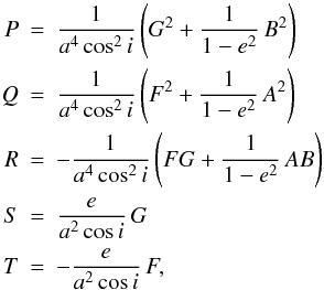 (A.2)where A,
B, F and G denote the familiar
Thiele-Innes constants:
(A.2)where A,
B, F and G denote the familiar
Thiele-Innes constants: 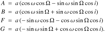 (A.3)
(A.3)
Note that our scaling factor is different from the one used by Smart (1930), because it is convenient for our purposes if the absolute term in Eq. (A.1) equals − 1.
In order to determine the semi-major and semi-minor axes of the apparent orbit, we
perform a principal axes transformation. We determine the eigenvalues
λ1 and λ2 of the matrix ℳ
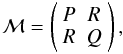 (A.4)which describes the binary quadratic form
A.1, as
(A.4)which describes the binary quadratic form
A.1, as
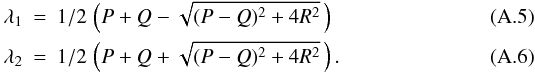 Inserting the eigenvalues into the
characteristic equation, we obtain
Inserting the eigenvalues into the
characteristic equation, we obtain  (A.7)which corresponds to Eq. (A.1) in a rotated and shifted coordinate
system. From Eq. (A.7) we immediately
determine the semi-major axis aapp and the semi-minor axis
bapp of the apparent orbit as
(A.7)which corresponds to Eq. (A.1) in a rotated and shifted coordinate
system. From Eq. (A.7) we immediately
determine the semi-major axis aapp and the semi-minor axis
bapp of the apparent orbit as
 (A.8)The astrometric signature
α then directly corresponds to the semi-major axis of the apparent
orbit, aapp, converted to angular units with the help of the
parallax ϖ:
(A.8)The astrometric signature
α then directly corresponds to the semi-major axis of the apparent
orbit, aapp, converted to angular units with the help of the
parallax ϖ: ![\appendix \setcounter{section}{1} \begin{equation} \alpha \mathrm{[mas]} = a_{\mathrm{app}} \mathrm{[AU]} \cdot \varpi \mathrm{[mas]} . \end{equation}](/articles/aa/full_html/2011/03/aa15861-10/aa15861-10-eq160.png) (A.9)Astrometric measurements are sometimes only
performed in one dimension at a time; examples are Hipparcos or PRIMA
(Delplancke 2008). In the case of PRIMA the
observing direction is given by the baseline orientation, which is flexible to a certain
degree. Thus, it might be advantageous for scheduling purposes to know the direction
where most of the astrometric signal can be expected, i.e. the orientation of the
apparent orbit. The rotation which leads from Eqs. (A.1) to (A.7) is
characterized by the rotation angle ϕ, which can be obtained from
(A.9)Astrometric measurements are sometimes only
performed in one dimension at a time; examples are Hipparcos or PRIMA
(Delplancke 2008). In the case of PRIMA the
observing direction is given by the baseline orientation, which is flexible to a certain
degree. Thus, it might be advantageous for scheduling purposes to know the direction
where most of the astrometric signal can be expected, i.e. the orientation of the
apparent orbit. The rotation which leads from Eqs. (A.1) to (A.7) is
characterized by the rotation angle ϕ, which can be obtained from
 (A.10)If the sign of R and
P − Q is taken into account, this returns an angle
ϕ in the range between 0 and 360 ° corresponding to the position
angle of the semi-major axis of the apparent orbit.
(A.10)If the sign of R and
P − Q is taken into account, this returns an angle
ϕ in the range between 0 and 360 ° corresponding to the position
angle of the semi-major axis of the apparent orbit.
Formally, the periastron is not defined for companions in circular orbits, but one can extend the usual definition by setting the longitude of the periastron to 0°, so that the periastron time will refer to the time when the observed stellar radial velocity curve reaches its maximum. For circular orbits, this occurs exactly a quarter of a period before (hypothetical) mid transit time.
Acknowledgments
We kindly thank Rainer Köhler for his help in the early phases of this project, and Viki Joergens as well as an anonymous referee for useful comments on the manuscript.
References
- Arriagada, P., Butler, R. P., Minniti, D., et al. 2010, ApJ, 711, 1229 [NASA ADS] [CrossRef] [Google Scholar]
- Bailey, J., Butler, R. P., Tinney, C. G., et al. 2009, ApJ, 690, 743 [Google Scholar]
- Barbieri, M., Alonso, R., Desidera, S., et al. 2009, A&A, 503, 601 [NASA ADS] [CrossRef] [EDP Sciences] [Google Scholar]
- Bean, J. L., McArthur, B. E., Benedict, G. F., et al. 2007, AJ, 134, 749 [Google Scholar]
- Bean, J. L., McArthur, B. E., Benedict, G. F., & Armstrong, A. 2008, ApJ, 672, 1202 [NASA ADS] [CrossRef] [MathSciNet] [Google Scholar]
- Benedict, G. F., McArthur, B. E., Forveille, T., et al. 2002, ApJ, 581, L115 [NASA ADS] [CrossRef] [Google Scholar]
- Benedict, G. F., McArthur, B. E., Gatewood, G., et al. 2006, AJ, 132, 2206 [NASA ADS] [CrossRef] [Google Scholar]
- Benedict, G. F., McArthur, B. E., Feast, M. W. et al. 2007, AJ, 133, 1810 [NASA ADS] [CrossRef] [Google Scholar]
- Benedict, G. F., McArthur, B. E., Napiwotzki, R., et al. 2009, AJ, 138, 1969 [NASA ADS] [CrossRef] [Google Scholar]
- Benedict, G. F., McArthur, B. E., Bean, J. L., et al. 2010, AJ, 139, 1844 [NASA ADS] [CrossRef] [Google Scholar]
- Bonfils, X., Mayor, M., Delfosse, X., et al. 2007, A&A, 474, 293 [NASA ADS] [CrossRef] [EDP Sciences] [Google Scholar]
- Bouchy, F., Mayor, M., Lovis, C., et al. 2009, A&A, 496, 527 [NASA ADS] [CrossRef] [EDP Sciences] [Google Scholar]
- Bowler, B. P., Johnson, J. A., Marcy, G. W., et al. 2010, ApJ, 709, 396 [NASA ADS] [CrossRef] [Google Scholar]
- Butler, R. P., Wright, J. T., Marcy, G. W., et al. 2006a, ApJ, 646, 505 [NASA ADS] [CrossRef] [Google Scholar]
- Butler, R. P., Johnson, J. A., Marcy, G. W., et al. 2006b, PASP, 118, 1685 [NASA ADS] [CrossRef] [Google Scholar]
- Casertano, S., Lattanzi, M. G., Sozzetti, A., et al. 2008, A&A, 482, 699 [NASA ADS] [CrossRef] [EDP Sciences] [Google Scholar]
- Cochran, W. D., Endl, M., Wittenmyer, R. A., & Bean, J. L. 2007, ApJ, 665, 1407 [Google Scholar]
- Correia, A. C. M., Udry, S., Mayor, M., et al. 2009, A&A, 496, 521 [NASA ADS] [CrossRef] [EDP Sciences] [Google Scholar]
- Correia, A. C. M., Couetdic, J., Laskar, J., et al. 2010, A&A, 511, A21 [NASA ADS] [CrossRef] [EDP Sciences] [Google Scholar]
- da Silva, R., Udry, S., Bouchy, F. et al. 2007, A&A, 473, 323 [NASA ADS] [CrossRef] [EDP Sciences] [Google Scholar]
- Delplancke, F. 2008, New Astron. Rev., 52, 199 [NASA ADS] [CrossRef] [Google Scholar]
- de Medeiros, J. R., Setiawan, J., Hatzes, A. P., et al. 2009, A&A, 504, 617 [NASA ADS] [CrossRef] [EDP Sciences] [Google Scholar]
- Desort, M., Lagrange, A.-M., Galland, F., et al. 2008, A&A, 491, 883 [NASA ADS] [CrossRef] [EDP Sciences] [Google Scholar]
- Döllinger, M. P., Hatzes, A. P., Pasquini, L., et al. 2007, A&A, 472, 649 [NASA ADS] [CrossRef] [EDP Sciences] [Google Scholar]
- Döllinger, M. P., Hatzes, A. P., Pasquini, L., et al. 2009a, A&A, 499, 935 [NASA ADS] [CrossRef] [EDP Sciences] [Google Scholar]
- Döllinger, M. P., Hatzes, A. P., Pasquini, L., Guenther, E. W., & Hartmann, M. 2009b, A&A, 505, 1311 [NASA ADS] [CrossRef] [EDP Sciences] [Google Scholar]
- Eggenberger, A., Udry, S., Chauvin, G., et al. 2007, A&A, 474, 273 [NASA ADS] [CrossRef] [EDP Sciences] [Google Scholar]
- ESA 1997, The Hipparcos and Tycho Catalogues, ESA SP-1200 [Google Scholar]
- Fischer, D. A., Vogt, S. S., Marcy, G. W., et al. 2007, ApJ, 669, 1336 [NASA ADS] [CrossRef] [Google Scholar]
- Fischer, D. A., Marcy, G. W., Butler, R. P., et al. 2008, ApJ, 675, 790 [NASA ADS] [CrossRef] [Google Scholar]
- Fischer, D., Driscoll, P., Isaacson, H., et al. 2009, ApJ, 703, 1545 [NASA ADS] [CrossRef] [Google Scholar]
- Forveille, T., Bonfils, X., Delfosse, X., et al. 2009, A&A, 493, 645 [NASA ADS] [CrossRef] [EDP Sciences] [Google Scholar]
- Guenther, E. W., Hartmann, M., Esposito, M., et al. 2009, A&A, 507, 1659 [NASA ADS] [CrossRef] [EDP Sciences] [Google Scholar]
- Halbwachs, J. L., Arenou, F., Mayor, M., Udry, S., & Queloz, D. 2000, A&A, 355, 581 [NASA ADS] [Google Scholar]
- Han, I., Lee, B. C., Kim, K. M., et al. 2010, A&A, 509, A24 [NASA ADS] [CrossRef] [EDP Sciences] [Google Scholar]
- Hatzes, A. P., Cochran, W. D., McArthur, B., et al. 2000, ApJ, 544, L145 [NASA ADS] [CrossRef] [Google Scholar]
- Hatzes, A. P., Guenther, E. W., Endl, M., et al. 2005, A&A, 437, 743 [NASA ADS] [CrossRef] [EDP Sciences] [Google Scholar]
- Hébrard, G., Udry, S., Lo Curto, G., et al. 2010a, A&A, 512, A46 [NASA ADS] [CrossRef] [EDP Sciences] [Google Scholar]
- Hébrard, G., Bonfils, X., Ségransan, D., et al. 2010b, A&A, 513, A69 [NASA ADS] [CrossRef] [EDP Sciences] [Google Scholar]
- Heintz, W. D. 1978, Double Stars, Geophysics and Astrophysics Monographs, (Dordrecht: D. Reidel Publishing Company), 15 [Google Scholar]
- Howard, A. W., Johnson, J. A., Marcy, G. W., et al. 2011, ApJ, 726, 73 [NASA ADS] [CrossRef] [Google Scholar]
- Johnson, J. A., Marcy, G. W., Fischer, D. A., et al. 2006, ApJ, 652, 1724 [NASA ADS] [CrossRef] [Google Scholar]
- Johnson, J. A., Fischer, D. A., Marcy, G. W., et al. 2007, ApJ, 665, 785 [NASA ADS] [CrossRef] [Google Scholar]
- Johnson, J. A., Howard, A. W., Marcy, G. W., et al. 2010, PASP, 122, 149 [NASA ADS] [Google Scholar]
- Jones, H. R. A., Butler, R. P., Tinney, C. G., et al. 2010, MNRAS, 403, 1703 [NASA ADS] [CrossRef] [Google Scholar]
- Kürster, M., Endl, M., & Reffert, S. 2008, A&A, 483, 869 [NASA ADS] [CrossRef] [EDP Sciences] [Google Scholar]
- Latham, D. W., Stefanik, R. P., Mazeh, T., Mayor, M., & Burki, G. 1989, Nature, 339, 38 [NASA ADS] [CrossRef] [Google Scholar]
- Launhardt, R., Henning, Th., Queloz, D., et al. 2008, Proc. SPIE 7013, 89 [Google Scholar]
- Liu, Y.-J., Sato, B., Zhao, G., et al. 2008, ApJ, 672, 553 , [NASA ADS] [CrossRef] [Google Scholar]
- Liu, Y.-J., Sato, B., Zhao, G., & Ando, H. 2009, Research Astron. Astrophys., 9, 1 [Google Scholar]
- Loeillet, B., Shporer, A., Bouchy, F., et al. 2008, A&A, 481, 529 [NASA ADS] [CrossRef] [EDP Sciences] [Google Scholar]
- López-Morales, M., Butler, R. P., Fischer, D. A., et al. 2008, AJ, 136, 1901 [NASA ADS] [CrossRef] [Google Scholar]
- Lovis, C., Mayor, M., Pepe, F., et al. 2006, Nature, 441, 305 [NASA ADS] [CrossRef] [PubMed] [Google Scholar]
- Martioli, E., McArthur, B. E., Benedict, G. F., et al. 2010, ApJ, 708, 625 [NASA ADS] [CrossRef] [Google Scholar]
- Mayor, M., Queloz, D., Udry, S., & Halbwachs, J.-L. 1997, Astronomical and Biochemical Origins and the Search for Life in the Universe, IAU Colloq., 161, 313 [NASA ADS] [Google Scholar]
- Mayor, M., Bonfils, X., Forveille, T., et al. 2009a, A&A, 507, 487 [NASA ADS] [CrossRef] [EDP Sciences] [Google Scholar]
- Mayor, M., Udry, S., Lovis, C., et al. 2009b, A&A, 493, 639 [NASA ADS] [CrossRef] [EDP Sciences] [Google Scholar]
- Mazeh, T., Zucker, S., dal la Torre, A., & van Leeuwen, F. 1999, ApJ, 522, L149 [NASA ADS] [CrossRef] [Google Scholar]
- McArthur, B. E., Endl, M., Cochran, W. D., et al. 2004, ApJ, 614, L81 [NASA ADS] [CrossRef] [Google Scholar]
- McArthur, B. E., Benedict, G. F., Barnes, R., et al. 2010, ApJ, 715, 1203 [NASA ADS] [CrossRef] [Google Scholar]
- McGrath, M. A., Nelan, E., Black, D. C., et al. 2002, ApJ, 564, L27 [NASA ADS] [CrossRef] [MathSciNet] [Google Scholar]
- Melo, C., Santos, N. C., Gieren, W., et al. 2007, A&A, 467, 721 [NASA ADS] [CrossRef] [EDP Sciences] [Google Scholar]
- Minniti, D., Butler, R. P., López-Morales, M., et al. 2009, ApJ, 693, 1424 [NASA ADS] [CrossRef] [Google Scholar]
- Moutou, C., Mayor, M., Lo Curto, G., et al. 2009, A&A, 496, 513 [NASA ADS] [CrossRef] [EDP Sciences] [Google Scholar]
- Naef, D., Latham, D. W., Mayor, M., et al. 2001, A&A, 375, L27 [NASA ADS] [CrossRef] [EDP Sciences] [Google Scholar]
- Naef, D., Mayor, M., Benz, D., et al. 2007, A&A, 470, 721 [NASA ADS] [CrossRef] [EDP Sciences] [Google Scholar]
- Niedzielski, A., Goździewski, K., Wolszczan, A., et al. 2009a, ApJ, 693, 276 [NASA ADS] [CrossRef] [Google Scholar]
- Niedzielski, A., Nowak, G., Adamów, M., & Wolszczan, A. 2009b, ApJ, 707, 768 [NASA ADS] [CrossRef] [Google Scholar]
- Noyes, R.W., Jha, S., Korzennik, S. G., Krockenberger, M., Nisenson, P., et al. 1997, ApJ, 483, L111 [NASA ADS] [CrossRef] [Google Scholar]
- O’Toole, S. J., Butler, R. P., Tinney, C. G., et al. 2007, ApJ, 660, 1636 [NASA ADS] [CrossRef] [Google Scholar]
- O’Toole, S. J., Tinney, C. G., Butler, R. P., et al. 2009, ApJ, 697, 1263 [NASA ADS] [CrossRef] [Google Scholar]
- Patel, S. G., Vogt, S. S., Marcy, G. W., et al. 2007, ApJ, 665, 744 [Google Scholar]
- Peek, K. M. G., Johnson, J. A., Fischer, D. A., et al. 2009, PASP, 121, 613 [NASA ADS] [CrossRef] [Google Scholar]
- Pepe, F., Correia, A. C. M., Mayor, M., et al. 2007, A&A, 462, 769 [NASA ADS] [CrossRef] [EDP Sciences] [Google Scholar]
- Perryman, M. A. C., Lindegren, L., Arenou, F., et al. 1996, A&A, 310, L21 [NASA ADS] [Google Scholar]
- Pourbaix, D., & Jorissen, A. 2000, A&AS, 145, 161 [NASA ADS] [CrossRef] [EDP Sciences] [Google Scholar]
- Pravdo, S. H., Shaklan, S. B., & Lloyd, J. 2005, ApJ, 630, 528 [NASA ADS] [CrossRef] [Google Scholar]
- Quirrenbach, A., et al. 1998, Proc. SPIE, 3350, 807 [NASA ADS] [CrossRef] [Google Scholar]
- Reffert, S., & Quirrenbach, A. 2006, A&A, 449, 699 [NASA ADS] [CrossRef] [EDP Sciences] [Google Scholar]
- Reffert, S., Quirrenbach, A., Mitchell, D. S., et al. 2006, ApJ, 652, 661 [NASA ADS] [CrossRef] [Google Scholar]
- Rivera, E. J., Butler, R. P., Vogt, S. S., et al. 2010, ApJ, 708, 1492 [NASA ADS] [CrossRef] [Google Scholar]
- Robinson, S. E., Laughlin, G., Vogt, S. S., et al. 2007, ApJ, 670, 1391 [NASA ADS] [CrossRef] [Google Scholar]
- Santos, N. C., Udry, S., Bouchy, F., et al. 2008, A&A, 487, 369 [NASA ADS] [CrossRef] [EDP Sciences] [Google Scholar]
- Santos, N. C., Mayor, M., Benz, W., et al. 2010, A&A, 512, A47 [NASA ADS] [CrossRef] [EDP Sciences] [Google Scholar]
- Sato, B., Izumiura, H., Toyota, E., et al. 2007, ApJ, 661, 527 [NASA ADS] [CrossRef] [Google Scholar]
- Sato, B., Izumiura, H., Toyota, E., et al. 2008a, PASJ, 60, 539 [NASA ADS] [Google Scholar]
- Sato, B., Toyota, E., Omiya, M., et al. 2008b, PASJ, 60, 1317 [NASA ADS] [Google Scholar]
- Sato, B., Fischer, D. A., Ida, S., et al. 2009, ApJ, 703, 671 [NASA ADS] [CrossRef] [Google Scholar]
- Ségransan, D., Udry, S., Mayor, M., et al. 2010, A&A, 511, A45 [NASA ADS] [CrossRef] [EDP Sciences] [Google Scholar]
- Setiawan, J., Henning, T., Launhardt, R., et al. 2008, Nature, 451, 38 [NASA ADS] [CrossRef] [PubMed] [Google Scholar]
- Smart, W. M. 1930, MNRAS, 90, 534 [NASA ADS] [Google Scholar]
- Sozzetti, A., & Desidera, S. 2010, A&A, 509, A103 [NASA ADS] [CrossRef] [EDP Sciences] [Google Scholar]
- Tamuz, O., Ségransan, D., Udry, S., et al. 2008, A&A, 480, L33 [NASA ADS] [CrossRef] [EDP Sciences] [Google Scholar]
- Tinney, C. G., Butler, R. P., Marcy, G. W., et al. 2001, ApJ, 551, 507 [NASA ADS] [CrossRef] [Google Scholar]
- Tokovinin, A. A., Duquennoy, A., Halbwachs, J.-L., & Mayor, M. 1994, A&A, 282, 831 [NASA ADS] [Google Scholar]
- Tokovinin, A., Thomas, S., Sterzik, M., & Udry, S. 2006, A&A, 450, 681 [NASA ADS] [CrossRef] [EDP Sciences] [Google Scholar]
- Udry, S., Mayor, M., Benz, W., et al. 2006, A&A, 447, 361 [NASA ADS] [CrossRef] [EDP Sciences] [Google Scholar]
- Unwin, S. C., Shao, M., Tanner, A. M., et al. 2008, PASP, 120, 38 [NASA ADS] [CrossRef] [Google Scholar]
- Valenti, J. A., Fischer, D., Marcy, G. W., et al. 2009, ApJ, 702, 989 [NASA ADS] [CrossRef] [Google Scholar]
- van Leeuwen, F. 2007a, Hipparcos, the New Reduction of the Raw Data, Astrophysics and Space Science Library, (Dordrecht: Springer), 350 [Google Scholar]
- van Leeuwen, F. 2007b, A&A, 474, 653 [NASA ADS] [CrossRef] [EDP Sciences] [Google Scholar]
- Vogt, S. S., Butler, R. P., Marcy, G. W., et al. 2002, ApJ, 568, 352 [NASA ADS] [CrossRef] [Google Scholar]
- Vogt, S. S., Wittenmyer, R. A., Butler, R. P., et al. 2010, ApJ, 708, 1366 [NASA ADS] [CrossRef] [Google Scholar]
- Walker, G. A. H., Walker, A. R., Irwin, A. W., et al. 1995, Icarus, 116, 359 [NASA ADS] [CrossRef] [Google Scholar]
- Wittenmyer, R. A., Endl, M., Cochran, W. D., Levison, H. F., & Henry, G. W. 2009, ApJS, 182, 97 [NASA ADS] [CrossRef] [Google Scholar]
- Wittenmyer, R. A., Endl, M., Cochran, W. D., et al. 2009, AJ, 137, 3529 [Google Scholar]
- Wright, J. T., & Howard, A. W. 2009, ApJS, 182, 205 [NASA ADS] [CrossRef] [Google Scholar]
- Wright, J. T., Marcy, G. W., Fischer, D. A., et al. 2007, ApJ, 657, 533 [NASA ADS] [CrossRef] [Google Scholar]
- Wright, J. T., Marcy, G. W., Butler, R. P., et al. 2008, ApJ, 683, L63 [NASA ADS] [CrossRef] [Google Scholar]
- Wright, J. T., Upadhyay, S., Marcy, G. W., et al. 2009a, ApJ, 693, 1084 [NASA ADS] [CrossRef] [Google Scholar]
- Wright, J. T., Fischer, D. A., Ford, E. B., et al. 2009b, ApJ, 699, L97 [NASA ADS] [CrossRef] [Google Scholar]
- Zucker, S., & Mazeh, T. 2000, ApJ, 531, L67 [NASA ADS] [CrossRef] [MathSciNet] [PubMed] [Google Scholar]
- Zucker, S., & Mazeh, T. 2001, ApJ, 562, 549 [NASA ADS] [CrossRef] [Google Scholar]
All Tables
Best fit inclinations, ascending nodes and companion masses for stars where the astrometric orbit could be detected.
Corrections (first rows) and final resulting values (second rows) of the five standard astrometric parameters (mean positions, parallax, proper motions) for the case where the astrometric modeling of the observations includes the effect of an orbiting companion.
Upper mass limits for substellar companion candidates detected via radial velocities.
All Figures
|
Fig. 1 Illustration of abscissa residuals from Hipparcos along with the astrometric orbit as fitted for ϵ Eri. The two panels in the top row show the abscissa residuals (colored dots) with respect to the standard astrometric model without orbiting companion (upper left) and with respect to a model (solid line) which includes the companion (upper right). The colored lines indicate the direction which was not measured and along which the dots are allowed to slide in the adjustment process; the actual abscissa measurement is perpendicular to that line. Color indicates orbital phase. The two panels in the bottom row show only one dimension each as a function of time. The solid line is the orbital model as in the upper panels, while the small grey dots are the individual abscissa residuals. The big black dots are averages of abscissa residuals taken very closely in time. The information about the orientation of the abscissa residuals is missing in the panels in the bottom row. |
| In the text | |
|
Fig. 2 Illustration of the allowed 3σ range of the companion mass for all stars from Table 1 for which the derived upper mass limit from Hipparcos corresponds to less than 85 MJup, i.e. for all 84 stars for which the substellar nature could be confirmed by Hipparcos. The lower mass limit usually corresponds to the lower mass limit m2 sini from the radial velocity fit, except for the few cases where the astrometry yields a tighter lower mass limit by excluding the inclination of 90° from the 3σ confidence region (HD 87883 b, HD 114783 b and γ Cep b). The upper mass limit always comes from the Hipparcos astrometry, according to Table 1. |
| In the text | |
|
Fig. 3 Illustration of the χ2 maps for those 20 stars for which the astrometric orbit could be detected in the Hipparcos data, as a function of inclination and ascending node. The contours show the 1σ, 2σ and 3σ confidence regions in both parameters jointly. Please note that for ρ CrB b the allowed range in inclination is so small that it is barely visible in this representation; the corresponding data can be found in Table 2. |
| In the text | |
Current usage metrics show cumulative count of Article Views (full-text article views including HTML views, PDF and ePub downloads, according to the available data) and Abstracts Views on Vision4Press platform.
Data correspond to usage on the plateform after 2015. The current usage metrics is available 48-96 hours after online publication and is updated daily on week days.
Initial download of the metrics may take a while.