| Issue |
A&A
Volume 527, March 2011
|
|
|---|---|---|
| Article Number | A32 | |
| Number of page(s) | 21 | |
| Section | Interstellar and circumstellar matter | |
| DOI | https://doi.org/10.1051/0004-6361/201015543 | |
| Published online | 21 January 2011 | |
Different evolutionary stages in the massive star-forming region S255 complex
1
Purple Mountain Observatory, Chinese Academy of Sciences,
210008
Nanjing,
PR China
e-mail: ywang@pmo.ac.cn
2
Max-Plank-Institute for Astronomy, Königstuhl 17, 69117
Heidelberg,
Germany
3
Graduate University of the Chinese Academy of Sciences,
19A Yuquan Road, Shijingshan
District, 100049
Beijing, PR
China
4
Centro de Astrobiología (CSIC-INTA), Ctra. de Torrejón a Ajalvir
km-4, 28850 Torrejón de Ardoz, Madrid, Spain
5
Instituut voor Sterrenkunde, Katholieke Universiteit Leuven,
Celestijnenlaan
200D, 3001
Leuven,
Belgium
6
Laboratoire d’Astrophysique de Marseille, UMR6110 CNRS,
38 rue F.
Joliot-Curie, 13388
Marseille,
France
7
National Astronomical Observatory of Japan, and GUAS, National Institutes of Natural
Sciences,
Japan
Received: 6 August 2010
Accepted: 11 November 2010
Aims. Massive stars form in clusters, and they are often found in different evolutionary stages located close to each other. To understand evolutionary and environmental effects during the formation of high-mass stars, we observed three regions of massive star formation at different evolutionary stages, and all are found that in the same natal molecular cloud.
Methods. The three regions, S255IR, S255N, and S255S, were observed at 1.3 mm with the submillimeter array (SMA), and follow-up short spacing information was obtained with the IRAM 30 m telescope. Near infrared (NIR) H + K-band spectra and continuum observations were taken for S255IR with VLT-SINFONI to study the different stellar populations in this region.
Results. This combination of millimeter (mm) and near infrared data allow us to characterize different stellar populations within the young forming cluster in detail. While we find multiple mm continuum sources toward all regions, their outflow, disk, and chemical properties vary considerably. The most evolved source S255IR exhibits a collimated bipolar outflow visible in CO and H2 emission, and the outflows from the youngest region S255S are still small and fairly confined in the regions of the mm continuum peaks. Also the chemistry toward S255IR is the most evolved, exhibiting strong emission from complex molecules, while much fewer molecular lines are detected in S255N, and in S255S we detect only CO isotopologues and SO lines. Also, rotational structures are found toward S255N and S255IR. Furthermore, a comparison of the NIR SINFONI and mm data from S255IR clearly reveal two different (proto) stellar populations with an estimated age difference of approximately 1 Myr.
Conclusions. A multiwavelength spectroscopy and mapping study reveals different evolutionary phases of the star formation regions. We propose the triggered outside-in collapse star formation scenario for the bigger picture and the fragmentation scenario for S255IR.
Key words: stars: formation / ISM: jets and outflows / ISM: molecules / stars: early-type / Hertzsprung-Russell and C-M diagrams / ISM: individual objects: S255
© ESO, 2011
1. Introduction
Massive stars (M > 8 M⊙) are one of the paramount components in the evolution of the universe, yet their formation is significantly less well understood than for their low-mass counterparts. S255IR is a famous massive star formation complex at a distance of  kpc (Rygl et al. 2010), embraced by the Sharpless regions S255 and S257 that are already evolved HII regions. The SCUBA 850 μm observation (Di Francesco et al. 2008; Klein et al. 2005) shows three main continuum sources: G192.60-MM2 (Minier et al. 2005) lies in the center region S255IR, and two additional mm continuum peak, G192.60-MM1 (Minier et al. 2005) and G192.60-MM3 (Minier et al. 2005), lie toward the northern region S255N and southern region S255S, respectively (Fig. 1).
The central region S255IR: the central IRAS source with a luminosity of 5 × 10⁴L⊙ (Minier et al. 2005) harbors three UCHII regions (Snell & Bally 1986) that are associated with Class II CH3OH and H2O maser emission (Goddi et al. 2007), which indicate the presence of massive young stellar objects. The luminosity would be 2 × 10⁴L⊙ if we apply the new distance of 1.59 kpc. The region hosts a cluster of low-mass sources that is surrounded by a shocked bubble of H2 gas (Ojha et al. 2006; Miralles et al. 1997). Tamura et al. (1991) resolved the central near infrared source into two compact sources, NIRS 1 and NIRS 3. Furthermore, Minier et al. (2007) report HCO+ infall signatures toward this region. In the mid-infrared, Longmore et al. (2006) resolved a massive proto-binary, which coincides with NIRS 1 and NIRS 3 (Fig. 3). And NIRS 1 has been identified as a massive disk candidate by near-infrared polarization observations (Jiang et al. 2008; see also Simpson et al. 2009, for a different interpretation).
 |
Fig. 1 SPITZER IRAC 4.5 μm image (Chavarría et al. 2008) overlaid with SCUBA 850 μm contours (Di Francesco et al. 2008; Klein et al. 2005). In the upper panel, the gray scale is the SPITZER IRAC 4.5 μm image, the black contours are the NVSS 1.4 GHz emission and the green contours are the SCUBA 850 μm continuum. In the bottom left panel, the gray scale is the SPITZER MIPS 24 μm image, the contours are the SCUBA 850 μm continuum, the three dashed circles mark the primary beam of our SMA observations. In the bottom right panel, the gray scale is the SPITZER MIPS 70 μm image, the contours and the circles are the same as the ones in the left panel. The contour levels of the NVSS start at 10σ (1σ = 0.6 mJy beam-1) in steps of 5σ. For the SCUBA 850 μm, the contour levels start at 10σ (1σ = 0.1 Jy beam-1) with a step of 10σ. The SPITZER/IRAC post-bcd data processed with pipeline version S18.7.0 and the MIPS post-bcd data processed with pipeline version S17.2.0 have been downloaded from the SPITZER archive to create these images. |
The northern region S255N: this region with 105L⊙ (Minier et al. 2005) also hosts a UCHII region G192.584-0.041 (Kurtz et al. 1994), as well as Class I CH3OH and H2O maser emission (Kurtz et al. 2004; Cyganowski et al. 2007), which indicate the presence of the massive young stellar objects. The luminosity would be 4 × 10⁴L⊙ if we apply the new distance of 1.59 kpc. The recent Submillimeter Array (SMA) observations toward that region at a spatial resolution of 3.6′′ resolved three mm sources and strong molecular line emission, and none of the sources is associated with NIR point source (Cyganowski et al. 2007). Outflow activity is shown by various tracers from shocked H2 emission via cm continuum and SiO emission (Miralles et al. 1997; Cyganowski et al. 2007), and global infall was reported by Minier et al. (2007).
The southern region S255S: this subsource is the least studied so far. It exhibits strong mm continuum emission (Fig. 1) but no other sign of active star formation yet, such as near infrared and mid infrared emissions. Therefore, it has been proposed that it is in a pre-stellar phase of the evolutionary sequence (Minier et al. 2007).
While G192.60-MM2 in S255IR still shows signs of active star formation, it is associated with an NIR cluster and appears to be the most evolved one of the three region. G192.60-MM1 in S255N has similar luminosity, and G192.60-MM3 is S255S is a high-mass starless core candidate. Therefore, S255 complex is the ideal candidate source to simultaneously investigate several sites of massive star formation at different evolutionary stages within the same larger scale environment.
2. Observations and data reductions
2.1. Submillimeter Array observations
The S255 complex was observed with three fields with the SMA on November 3, 2008 in the compact configuration with seven antennas and on February 8, February 17, 2009 in the extended configuration with eight antennas, and February 13 in the extended configuration with seven antennas. The phase centers of the fields, which are known as S255IR, S255N, and S255S, were RA 06h12m54.019s Dec + 17°59′23.10′′ (J2000.0), RA 06h12m53.669s Dec + 18°00′26.90′′ (J2000.0) and RA 06h12m56.58s Dec + 17°58′32.80′′ (J2000.0), respectively. The SMA has two spectral sidebands, both 2 GHz wide and separated by 10 GHz. The receivers were tuned to 230.538 GHz in the upper sideband (vlsr = 10 km s-1) with a maximum spectral resolution of 0.53 km s-1. The weather on February 8 and February 13 was mediocre with zenith opacities τ(225 GHz) more than 0.2 as measured by the Caltech Submillimeter Observatory (CSO). But the weather on November 3, 2008 and February 17, 2009 was good with zenith opacities τ (225 GHz) around 0.1, so we only used the data observed on these two days. For the compact configuration on the November 3, 2008 bandpass was derived from the quasar 3c454.3 observations. Phase and amplitude were calibrated with regularly interleaved observations of the quasar 0530+135 (11.4° from the source). The flux calibration was derived from Uranus observations, and the flux scale is estimated to be accurate within 20%. For the extended configuration on the February 17, 2009 bandpass was derived from the quasar 3c273 observations. Phase and amplitude were calibrated with regularly interleaved observations of the quasar 0530+135. Because of the lack of flux calibrator observations, the flux was estimated by the SMA calibrator database for the gain calibrator to be accurate within 20%. We merged the two configuration data set, applied different robust parameters for the continuum and line data, and got the synthesized beam sizes between 1.4′′ × 1.1′′ (PA 86°) and 1.9′′ × 1.6′′ (PA 77°), respectively. The 3σ rms of 1.3 mm continuum image is ~4.5 mJy beam-1, and the 3σ rms of the line data is 0.14 Jy beam-1 at 2 km s-1 spectral resolution. The flagging and calibration was done with the IDL superset MIR (Scoville et al. 1993), which was originally developed for the Owens Valley Radio Observatory and adapted for the SMA1. The imaging and data analysis were conducted in MIRIAD (Sault et al. 1995).
2.2. Short spacing from the IRAM 30 m
To complement the CO(2−1) observations with the missing short-spacing information and to investigate the large-scale general outflow properties to find the connection of the three regions, we observed them with the HERA array at the IRAM 30 m telescope on November 10, 2009. The 12CO(2−1) line at 230.5 GHz and 13CO(2−1) line at 220.4 GHz were observed in the on-the-fly mode. We mapped the whole region with a size of 5′ × 3′ centered at RA 06h12m54.02s Dec + 17°59′23.10′′ (J2000.0). The sampling interval was 3.5′′, a bit better than Nyquist-sampling to minimize beam-smearing effects. The region was scanned two times in the declination and right ascension direction, respectively, in order to reduce effects of the scanning process. The spectra were calibrated with CLASS, which is part of the GILDAS software package, then the declination and right ascension scans were combined with the plait algorithm in GREG, which is another component of the GILDAS package. The 12CO data has a beam size of 11′′, and the rms noise level of the corrected Tmb is around 0.23 K at 0.6 km s-1 spectral resolution. The 13CO has the same beam size, but the rms noise is 0.12 K at 0.6 km s-1 spectral resolution.
After reducing the 30 m data separately, single-dish 12CO and 13CO data were converted to visibilities and then combined with the SMA data using MIRIAD package task UVMODEL. With different uv-range selections, the synthesized beam of the combined data varies from 2.1′′ × 1.8′′ (PA − 84°) to 11.1′′ × 10.7′′ (PA − 74°).
2.3. VLT-SINFONI integral field spectroscopy observations
Near infrared H- and K-band observations were performed using the integral field instrument SINFONI (Eisenhauer et al. 2003; Bonnet et al. 2004) on UT4 (Yepun) of the VLT at Paranal, Chile. The observations of S255IR were performed in service mode on February 8, February 12, February 13, and March 29, 2007. The non-AO mode of SINFONI was used in combination with the setting that provides the widest field of view (8′′ × 8′′) with a spatial resolution of 0.25′′ per slitlet. The typical seeing during the observations was 0.7′′ in K-band. The H+K grating was used, covering these bands with a resolution of R = 1500 in a single exposure.
S255IR was observed with a detector integration time (DIT) of 30 seconds per pointing. The observations were centered on the central near infrared source NIRS 1 at coordinates: RA 06h12m53.85s Dec + 17°59′23.71′′ (J2000.0). We observed this area with SINFONI using a raster pattern, covering every location in the cluster at least twice, resulting in an effective integration time of 60 s per location in the field. The offset in the east-west direction was 4′′ (i.e. half the FOV of the detector) and the offset in the north-south direction was 6.75′′, resulting in a total observation field of 70′′ × 70′′. A sky frame was taken every 3 min using the same DIT as the science observations. The sky positions were chosen based on existing NIR imaging in order to avoid contamination. Immediately after every science observation, a telluric standard star was observed, matching the airmass of the object as closely as possible.
 |
Fig. 2 Lower and upper sideband spectral vector-averaged over all baselines with a resolution of 2 km s-1 per channel. In the upper sideband image, the 12CO line in S255IR and S255N panels was not fully plotted, which goes to 11.6 Jy and 5.9 Jy, respectively. |
The data were reduced using the SPRED (version 1.37) software developed by the MPE SINFONI consortium (Schreiber et al. 2004; Abuter et al. 2006). The procedure described by Davies (2007) was applied to remove the OH line residuals. To calibrate the flux and remove the telluric absorption lines, the extracted spectrum of one standard star in each OB (OB1: Hip064656, OB2: Hip048128, OB3: Hip032108, OB4: Hip031899) is used. The flux calibration of the spectra uses the 2MASS (Cohen et al. 2003) magnitude of the standard stars (see Bik et al. 2010, for the details of the data reduction).
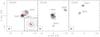 |
Fig. 3 The SMA 1.3 mm continuum map of S255IR, S255N, and S255S. contour levels start at 5σ in steps of 5σ in S255IR (1σ = 1.7 mJy/beam) and S255N (1σ = 1.6 mJy/beam) image and 3σ in S255S (1σ = 0.9 mJy/beam) image. The dotted contours are the negative features due to the missing flux. The synthesis beam is shown at the bottom left of each figure. In the S255IR panel, the asterisk marks the position of NIRS 3 and the right one marks NIRS 1 (Tamura et al. 1991). The inset is a zoom in the continuum image of the inner region of S255IR-SMA1 and the contour levels start at 5σ in steps of 10σ. The triangles are the water masers (Goddi et al. 2007) and the two open diamond mark the positions of two 6.7 GHz methanol masers detected by Xu et al. (2009). In S255N panel, the crosses mark the position of the Class I 44 GHz (70 − 61) A+ methanol masers detected by Kurtz et al. (2004) and the triangle is the water maser (Cyganowski et al. 2007). The (0, 0) point in each panel from left to right is RA 06h12m54.019s Dec 17°59′23.10′′ (J2000.0), RA 06h12m53.669s Dec + 18°00′26.90′′ (J2000.0) and RA 06h12m56.58s Dec + 17°58′32.80′′ (J2000.0), respectively. |
Millimeter continuum peak properties.
3. Results
3.1. Millimeter continuum emission
We averaged the apparently line-free parts of upper and lower sideband spectra of each region (presented in Fig. 2) and got the continuum images of the three regions shown in Fig. 3.
Assuming optical thin dust emission, we estimated the gas mass and column density of the continuum sources following the equations outlined in Hildebrand (1983) and Beuther et al. (2005a). We assumed a dust temperature of 40 K, grain size of 0.1 μm, grain mass density of 3 g cm3, gas-to-dust ratio of 100, and a grain emissivity index of 2 (corresponding to κ ≈ 0.3 for comparison of Ossenkopf & Henning 1994). The results are shown in Table 1. With the same set-up, we also calculated the gas mass and the column density of the SCUBA 850 μm (Di Francesco et al. 2008; Klein et al. 2005) continuum peaks shown in Table 2. To get the impression of how much flux we lost in the interferometer observations, we produced the SMA continuum map of the each region with the same beam size as the SCUBA 850 μm map (14′′ × 14′′, Di Francesco et al. 2008). We measured the continuum flux, calculated the gas mass, and compared the results with the ones in Table 2. The mass we obtained from the SMA observations for S255IR, S255N, and S255S is only 7.8%, 8.7%, and 2% of the SCUBA 850 μm measurements, respectively. Since our interferometer observations are not sensitive to spatial scales > 24′′ (the shortest base line =8.5 kλ), we filtered out the smoothly distributed large-scale halo and left only the compact cores. Also, that we filtered out more flux for the youngest region S255S indicates that at the earliest evolutionary stages the gas is more smoothly distributed than during later stages where the collapse produces more centrally condensed structures. Nevertheless, all derived column densities are close to or above the proposed threshold for high-mass star formation of 1 g cm-2 (Krumholz & McKee 2008).
SCUBA submillimeter continuum data.
S255IR.
The continuum image of S255IR is presented in the left hand panel of Fig. 3. We resolved two main continuum peaks (i.e. S255IR-SMA1 and S255IR-SMA2) and one unresolved subpeak (i.e. S255IR-SMA3) in this region. The stronger peak named as S255IR-SMA1 in the southeast coincides with the near-infrared source NIRS 3 (Tamura et al. 1991). S255IR-SMA1 coincides with a UCHII region (Snell & Bally 1986) generated by NIRS 3, and the inset in the S255IR panel in Fig. 3 shows that it is also associated with Class II CH3OH and H2O maser emissions (Goddi et al. 2007; Minier et al. 2000, 2005). An unresolved peak S255IR-SMA3 coincides with the near-infrared source NIRS 1 (Tamura et al. 1991), which lies 2.4′′ west of S255IR-SMA1 and has been identified as a massive disk candidate by NIR polarization observation (Jiang et al. 2008). These two continuum sources are both coincident with the mid-infrared massive proto-binary sources 1 and 2 identified by Longmore et al. (2006). S255IR-SMA2, which has never been detected before, is not associated with any infrared source and likely to be in a very young source. It also shows only a few lines, which will be discussed in detail in Sect. 3.2.
S255N.
The middle panel of Fig. 3 is the continuum image of S255N. The strongest peak named as S255N-SMA1, which coincides with the UCHII region G192.584-0.041 (Kurtz et al. 1994), is associated with Class I 44 GHz (70 − 61) A+ methanol masers, which are detected by Kurtz et al. (2004) and water maser (Cyganowski et al. 2007). All the methanol masers are distributed along the direction of the outflow (Fig. 10, see Sect. 3.3). S255N-SMA1 is also associated with centimeter continuum emission (Cyganowski et al. 2007), which shows an elongation aligned with the outflow (Fig. 10, left panel). However, all three continuum sources in S255N have no corresponding near-infrared point sources.
 |
Fig. 4 S255IR CH3OH line integrated intensity images with the SMA 1.3 mm continuum emission in the background. Contour levels start at 3σ with 2σ/level. For the top panels, the σ of the contours in each panel, from left to right, is 12, 15, 11 mJy beam-1, respectively, and for the bottom panels is 12, 14, 15 mJy beam-1, respectively. The dotted contours are the negative feature. The integral velocity ranges are shown in the bottom left corner of each panel in km s-1. The synthesized beams are shown in the bottom left corner of each panel. The (0, 0) point in each panel is RA 06h12m54.019s Dec + 17°59′23.10′′ (J2000.0). |
S255S.
The right hand panel of Fig. 3 presents the continuum image of S255S. There are no near infrared sources or mid infrared peaks (SPITZER MIPS 24 μm and 70 μm, Fig. 1) that are associated with these two sources. Meanwhile, the gas mass is only 2% of the SCUBA 850 μm measurements, which indicates that the gas in this region is at an early stage and smoothly distributed. All these features indicate that S255S is an extremely young region.
Observed lines in S255IR.
 |
Fig. 5 S255IR molecular line integrated intensity contour with the SMA 1.3 mm continuum emission in the background. All the contour levels start at 3σ. The contour step is 3σ in SO (1σ = 22 mJy beam-1), HCOOH (1σ = 10 mJy beam-1), HCOOCH3 (1σ = 12 mJy beam-1), C18O (1σ = 16 mJy beam-1), CH3CN (1σ = 11 mJy beam-1) and HNCO (1σ = 13 mJy beam-1) images, and 1σ in OCS (1σ = 13 mJy beam-1) and 13CS (1σ = 11 mJy beam-1) image. The dotted contours are the negative features with the same contours as the positive ones in each panel. The integral velocity ranges are shown in the bottom left corner of each panel in km s-1. The synthesized beams are shown in the bottom left corner of each panel. We only plotted the line for CH3CN and (100,10 − 90,9) line for HNCO. The (0, 0) point in each panel is RA 06h12m54.019s Dec + 17°59′23.10′′ (J2000.0). |
3.2. Spectral line emission
The observed spectra of lower sideband (LSB) and upper sideband (USB) of three region are shown in Fig. 2.
S255IR.
In S255IR, we detect 25 lines from 10 species. Besides three normal CO isotopologues, we also detect some sulfur-bearing species (SO, 34SO2, OCS, 13CS) and some dense gas molecules which are usually used to trace high-mass hot cores, such as CH3OH, CH3CN, and HCOOCH3 (Nomura & Millar 2004; Beuther et al. 2009; Sutton et al. 1985). All the lines we detected have lower energy levels Elower/k between 5.3 to 568 K (Table 3).
Figures 4 and 5 present the integrated line images of all species (except 34SO2, which is blended with CH3OH and too weak for imaging, and 12CO and 13CO will be discussed in detail in Sect. 3.3) with different transitions. Most lines show compact emission peaked at S255IR-SMA1, and only a few show emission at S255IR-SMA2. Several CH3OH lines (CH3OH(80,8 − 71,6)E, CH3OH(8 − 1,8 − 70,7)E, and CH3OH(32,2 − 41,4)E, in Fig. 4) exhibit extended emission towards S255IR-SMA2. The CH3OH(8 − 1,8 − 70,7)E line even extends to the northwest of S255IR-SMA1 following the direction of the blue-shifted outflow of S255IR-SMA1 (Fig. 8, see Sect. 3.3). We suggest that the particular (8−1,8 − 70,7)E line is due to the shock heating excited by the outflow, which could also be mixed up with some Class I methanol maser emission (Sutton et al. 2004; Sobolev et al. 2005; Kalenskii et al. 2002; Slysh et al. 2002). SO line emission associated with S255IR-SMA1 is elongated along the outflow and could be affected by the outflow. 13CS line emission forms a shell around S255IR-SMA1 (Fig. 5, similar shell-like C34S emission has also been found by Beuther et al. 2009). Only a few lines are associated with S255IR-SMA2, SO, C18O (Fig. 5) and several methanol lines (Fig. 4). S255IR-SMA2 appears to be chemically younger than S2555IRmm1. We extracted C18O spectra from these two continuum peaks. The spectrum toward S255IR-SMA1 shows two peaks and cannot be fitted by a single Gaussian profile; therefore, we calculated the FWZI (full width at zero intensity) of these two C18O spectra, which is 12 km s-1 and 6.8 km s-1 for S255IR-SMA1 and S255IR-SMA2, respectively. The difference of the line width also suggests that S255IR-SMA2 is at a younger evolutionary stage.
Observed lines in S255N.
 |
Fig. 6 S255N molecular line integrated intensity contour with the SMA 1.3 mm continuum emission in the background. All the contour levels start at 3σ. The contour step is 1σ in CH3OH(80,8 − 71,6)A- (1σ = 9 mJy beam-1) and CH3CN(, 1σ = 14 mJy beam-1) images, 2σ in 13CS (1σ = 25 mJy beam-1) image, 3σ in SO (1σ = 13 mJy beam-1) and CH3OH(81,8 − 70,7)E images, and 0.5σ in OCS (1σ = 10 mJy beam-1) image. The dotted contours are the negative features. The integral velocity ranges are shown in the bottom-left corner of each panel in km s-1. The synthesized beams are shown in the bottom left of each panel. The (0, 0) point in each panel is RA 06h12m53.669s Dec + 18°00′26.90′′ (J2000.0). |
S255N.
In S255N, we detected 10 lines from 6 species (12CO, SO, CH3OH, CH3CN, OCS, 13CS) and 2 additional CO isotopologues (13CO and C18O) with lower energy levels Elower/k between 5.3 to 65 K (Table 4). Figure 6 shows the integrated line images of all species (except three CO isotopologues, which will be discussed in Sects. 3.3 and 3.4). All the lines show a peak associated with S255N-SMA1, CH3OH and SO lines also show extended emission along the direction of the outflows (Fig. 10, see Sect. 3.3).
S255S.
In S255S, we detected 4 lines from two species (12CO and SO) and 2 additional CO isotopologues (13CO and C18O) with lower energy levels Elower/k between 5.3 to 24 K (Table 5), which again indicates that S255S is an extremely young and cold region. We measured the single dish 13CO line width toward the S255S SCUBA 850 μm continuum peak, and calculated the virial mass in this region, which is ~80 M⊙. The virial mass is lower than the mass we got from the SCUBA 850 μm measurement, which implies that S255S region will probably collapse.
Observed lines in S255S.
From the single-dish 13CO observations, we got the vlsr of the three regions, which are shown in Table 6. However, the vlsr of the high-mass mm cores in S255IR and S255N based on the interferometer observations is different from the one we got from the single-dish data. We extracted dense gas spectra, i.e. CH3OH for S255N-SMA1, CH3CN for S255IR-SMA1, and C18O for S255IR-SMA2, and then a Gaussian profile was fitted to get the vlsr of the cores. All the velocities are shown in Table 6. For S255S we cannot get a proper vlsr from the SMA observations due to the missing flux problem, so only the vlsr we got from 30 m observation is listed.
The vlsr measured with different telescopes.
3.3. The molecular outflows
After combining the single-dish 30 m data with the interferometer data, we integrated the line wing of 12CO and produced the outflow image of each region. Figure 7 shows the single-dish-only outflow map. While the northeast-southwest (NE-SW) outflow that is associated with S255IR is clearly shown in Fig. 7, the high-velocity outflow is also found in the S255N region; however, the direction of the outflow could not be defined well on single-dish outflow map. In the youngest region, S255S, the single-dish outflow map does not show much emission. We combined the SMA data and 30 m data to study the outflow properties.
 |
Fig. 7 The single-dish outflow map of the S255 complex. The blue-shifted outflow is shown in dashed contours with a velocity-integration regime of [−40, 0] km s-1, and the red one is shown in full contours with a velocity-integration regime of [16, 56] km s-1. The contours start at 4σ in steps of 5σ (1σ = 1.2 K km s-1). The three crosses mark the position of the three SCUBA 850 μm continuum sources. |
S255IR.
Figure 8 shows the combined SMA and 30 m outflow images of S255IR. The velocity-integration regime of the blue-shifted part is [−40, 0] km s-1 and [16, 56] km s-1 for red-shifted part. We selected different uv-ranges resulting in different resolutions. Although at different resolutions, the structure of the outflow changes a lot, the northeast-southwest (NE-SW) outflow is confirmed in all images (also reported by Miralles et al. 1997). In the bottom-left panel, the H2 jet-like sources (regions (a) and (b) in Fig. 19, see Sect. 3.6.1) also follow the NE-SW outflow direction. The water masers that are marked with triangles in the inset of S255IR panel in Fig. 3 also follow the direction of the outflow, which confirms that S255IR-SMA1 is the driving source of this NE-SW outflow. In all panels except the bottom-right two, the red-shifted part of the outflow bends a little toward NW, which might be a signature of the precessing jets. In the S255IR panel in Fig. 3, the water masers also follow the NE-SW direction. We believe that NIRS 3 is the driving source of this outflow. As we are applying different uv-range selections, two red-shifted outflow components show up out to the north and south of the continuum sources, respectively, and these two components are both only shown in the lower velocity regime, which is offset from the vlsr 10 to 20 km s-1. Finally, in the 30 m-only panel and Fig. 7, the red-shifted outflow component to the north of the continuum sources becomes connected with the component in S255N.
Figure 9 presents the position-velocity (pv) diagram of the molecular gas along the outflow. The diagram shows that the red- and blue-shifted outflow resembles the Hubble-law with increasing velocity at a longer distance from the outflow center, and the blue-shifted outflow also resembles the jet-bow-shock gas entrainment model (Arce et al. 2007).
S255N.
Figure 10 shows the combined SMA and 30 m outflow images of S255N. The velocity-integration regime of the blue-shifted part is [−44, 0] km s-1 and [16, 48] km s-1 for the red-shifted part. The northeast-southwest (NE-SW) outflow is shown clearly in the SMA and SMA combined with 30 m panels but is hardly seen in the 30 m-only panel. In the middle panel, the crosses mark the position of the Class I 44 GHz (70 − 61) A+ methanol masers detected by Kurtz et al. (2004) and the triangle is the water maser (Cyganowski et al. 2007). In the left hand panel, the background gray scale is VLA Q-band 3.6 cm continuum (Cyganowski et al. 2007) which shows a jet-like structure. All these features follow the NE-SW direction. Based on these features we confirm the direction of the main outflow as NE-SW. The red-shifted outflow to the north of S255N-SMA1 on the line (b) top left panel in Fig. 10 might be part of the outflow cavity, but we can not exclude the possibility of multiple outflows. The red-shifted gas at the bottom part of line (b) seems to be associated with S255N-SMA3 (the middle panel of Fig. 10), however, another blue-shifted feature at the southern part of the map shows up as the resolution changes. These two components both can also only be detected at the relatively lower velocity regime ~10 to 20 km s-1 offset from the vlsr.
 |
Fig. 8 S255IR 12CO(2−1) outflow images observed with IRAM 30 m telescope and the SMA. The blue-shifted outflow is shown in dashed contours with a velocity-integration regime of [−40, 0] km s-1, and the red one is shown in full contours with a velocity-integration regime of [16, 56] km s-1. The top left panel presents the SMA data only map, the bottom right one presents the IRAM 30 m data only map. The others are all combined SMA + 30 m data, which are inverted with different uv-range selections (shown in the top right of each panel in kλ) resulting in different beam sizes shown in the bottom left corner of each panel. All the 12CO emission contour levels start at 5σ in steps of 10σ. The dotted contours are the negative features and the stars mark the position of NIRS 3. In the bottom left panel, the background scale is SINFONI H2 line emission. The line in the SMA-only panel shows the pv-cut presented in Fig. 9, and the cross marks the central position of the line. In panel (0, 120), the SMA 1.3 mm continuum map is overplotted (black full contours), and the contours start at 5σ in steps of 5σ. In panel (0, 70), the same CH3OH (8−1,8 − 70,7)E integrated intensity map in Fig. 4 is over plotted in black full contours . The σ of the outflow data is shown in Table 7. The (0, 0) point in each panel is RA 06h12m54.019s Dec + 17°59′23.10′′ (J2000.0). |
Figure 11 presents the position-velocity (pv) diagrams of the molecular gas along the outflows. In the top panel, the pv-plot cut follows the direction of the VLA jet-like emission (Fig. 10, left panel, line a). The diagram shows that the high-velocity gas on the blue-shifted side remains very close to the outflow center, and the red-shifted part does not show the Hubble-law signature. But in the bottom panel, in which the pv-plot cut follows the direction of the two elongate red-shifted emission (Fig. 10, left panel, line b), the red-shifted northern side of the outflow resembles the Hubble-law. However, the red-shifted southern part of the outflow seems to have nothing to do with our S255N-SMA1 nor S255N-SMA3. The different blue/red pv-characteristics may be explained by the blue 12CO emission mainly tracing the jet-like component also visible in centimeter continuum emission, whereas the red 12CO emission traces mainly the cavity-like walls of the outflow or another outflow.
S255S.
Figure 12 presents the combined SMA and 30 m outflow images of S255S. The velocity-integration regime of the blue-shifted part is [−9, 1] km s-1 and [14, 32] km s-1 for the red-shifted part. All the panels except the 30 m-only one show two blue-shifted components and one red-shifted component. Although the line wing emission is less pronounced than for the other two regions, we clearly identify blue- and red-shifted 12CO emission associated with both mm peaks. The blue-shifted part in the south of the map is only detected in the 1 km s-1 ≥ v ≥ −6 km s-1, and the red-shifted part in the north of the map is only detected in the v ≤ 16 km s-1. Since the line wing emission does not extend to very high velocities, the outflow should not be oriented directly along the line of sight. Therefore, the small spatial extent of the outflow also indicates the youth of this region.
 |
Fig. 9 Position-velocity diagrams of S255IR for the 12CO(2 − 1) SMA-only outflow observations with a velocity resolution of 1 km s-1. The pv-diagram is in NE-SW direction with a PA of 75° from the N (the cut is marked in Fig. 8, top-left panel). The contour levels are from 10 to 90% from the peak emission (4.2 Jy beam-1) in steps of 10%. The vlsr at 7.7 km s-1 and the central position (marked by the cross in Fig. 8top-left panel) are marked by vertical and horizontal lines. |
Applying the method of Cabrit & Bertout (1990, 1992) we derived properties of the outflows such as outflow mass, outflow energy, and dynamical age. Since the SMA data suffer a lot from the missing flux problem, only the 30 m data are used in the calculations. These calculations assume that the 13CO(2−1)/12CO(2−1) line wing ratio is 0.1 (Choi et al. 1993; Levreault 1988; Beuther et al. 2002). The results are shown in Table 8. The dynamical age calculation depends on the tangent of the outflow’s inclination angle (with 0° being in the plane of the sky). Since we cannot get the inclination angle information of these sources, we assumed an inclination angle of 45° for all the dynamical age calculations. For S255N and S255S, the outflows are not clearly defined in the 30 m-only maps (Figs. 10 and 12). Therefore, we used with the SMA + 30 m map to determine the outflow sizes (see right panels of Figs. 10 and 12). For S255S, since we only detected one outflow lobe associated with each continuum source, we just extended the only lobe to the opposite side of the source to get the proper size and mass of the outflow.
3.4. Rotational structures
S255IR.
Figure 13 shows the velocity moment maps of HCOOCH3, CH3CN (k = 2) and C18O(2 − 1). In the velocity maps of HCOOCH3 and CH3CN (k = 2), we see a clear velocity gradient perpendicular to the outflow axis, which indicates there is a rotational structure. The C18O(2 − 1) velocity map shows a little different picture compared to the other ones. C18O traces a more diffuse gas than for the other two molecules. The C18O velocity map also shows a big velocity difference between S255IR-SMA1 and S255IR-SMA2.
 |
Fig. 10 S255N 12CO(2−1) outflow images observed with IRAM 30 m telescope and the SMA. The blue-shifted outflow is shown in dashed contours with a velocity-integration regime of [−44, 0] km s-1, and the red one is shown in full contours with a velocity-integration regime of [16, 48] km s-1. The left panel presents the SMA data only map, the right presents the IRAM 30 m data only map. The synthesized beam is shown in the bottom left corner of each panel. The middle one is combined SMA + 30 m data, the uv-range selection is shown in the top right of each panel in kλ. All the CO emission contour levels start at 5σ in steps of 6σ. The dotted contours are the negative features and the asterisks mark the position of continuum peaks. In the middle panel, the crosses mark the position of the Class I 44 GHz (70 − 61) A+ methanol masers detected by Kurtz et al. (2004) and the triangle is the water maser (Cyganowski et al. 2007). In the top left panel, the background gray scale is VLA Q-band continuum (Cyganowski et al. 2007) and the line shows the pv-cut presented in Fig. 11, which follows the masers direction and crosses the continuum peak. The arrow in the 30 m-only panel marks the outflow size we used to calculate the outflow physical parameters. The σ of the outflow data is shown in Table 7. The (0, 0) point in each panel is RA 06h12m53.669s Dec + 18°00′26.90′′ (J2000.0). |
 |
Fig. 11 Position-velocity diagrams of S255N for the 12CO(2 − 1) SMA-only outflow observations with a velocity resolution of 1 km s-1. The top panel is the pv-plot in NE-SW direction with a PA of 54° from the N (the cut is marked as the line a in Fig. 10, left panel), and the bottom panel is the pv-plot in NW-SE direction with a PA of 7° from the N. (The cut is marked as the line b in Fig. 10, left panel.) The contour levels are from 10 to 90% from the peak emission (4.15 Jy beam-1 in the top panel and 2.82 Jy beam-1 in the bottom panel) in steps of 10%. The vlsr at 8.6 km s-1 and the central position (i.e. the S255N-SMA1 position in the top panel and the cross point of lines a and b in Fig. 10 top-left panel in the bottom panel) are marked by horizontal and vertical lines. |
Figure 14 shows the position-velocity diagrams of the HCOOCH3 and C18O(2 − 1) emission. The cuts, which are shown in Fig. 13, go through the peak of the dust continuum and have position angles perpendicular to the direction of the outflow presented in Fig. 8. The pv-diagram of HCOOCH3 shows that the rotational structure is not in Keplerian motion, hence it may be just a rotating and infalling core similar to the toroids described by Cesaroni et al. (2007). The approximately 2.3′′ diameter of the rotational structure corresponds to 3700 AU at the given distance of 1.59 kpc. The pv-diagram of CH3CN (k = 2) has a similar structure to the one of HCOOCH3, thus we do not show it.
However, the picture is different for C18O, the pv-diagram shows a Keplerian-like rotation structure. The full line in the C18O panel shows a Keplerian rotation curve with a central mass of 28 M⊙, which is the mass of the whole continuum structure in S255IR covering both mm peaks. For a more detailed discussion, see Sect. 4.3.
S255N.
Figure 15 shows the velocity moment maps of CH3OH(8 − 1,8 − 70,7), CH3OH (80,8 − 71,6) and C18O(2 − 1). The C18O velocity map shows a complicated velocity structure, the velocity gradient is neither aligned with nor orthogonal to the outflow orientation. Because C18O is an isotopologue of 12CO, it may be influenced by infall and the outflow. Methanol is well known as a molecule that traces cores, shocks, and masers in star formation regions (Jørgensen et al. 2004; Beuther et al. 2005b; Sobolev et al. 2007). It has also been reported as a low-mass disk tracer (Goldsmith et al. 1999). In the velocity maps of the two methanol transitions (left and middle panels of Fig. 15), we see a velocity gradient perpendicular to the outflow axis, which indicates a rotational structure.
Figure 16 shows the position-velocity diagram of the (80,8 − 71,6) methanol line emission, and the pv-diagram of the other methanol transition shows the similar velocity structure. The cuts go through the peak of the dust continuum and have position angles perpendicular to the direction of the outflow (Fig. 15). The pv-diagram shows that the rotational structure is not Keplerian. The structure has a size of 4.4′′ corresponding to 7000 AU at the given distance of 1.59 kpc. It has a narrow velocity range of 3 km s-1, and may likely be a large rotating and infalling core similar to the toroids described by Cesaroni et al. (2007).
There are two low-velocity components in the NE and SW of the continuum peak in the methanol velocity maps, which coincide with the outflow. They may be caused by the shock heating emission, and the line profile is consistent with both thermal and maser emission (Sutton et al. 2004; Sobolev et al. 2005; Kalenskii et al. 2002; Slysh et al. 2002).
3.5. Temperature from CH3CN(12k − 11k) in S255IR
Since we detected 7 lines of the CH3CN(12k − 11k) k-ladder with k = 0...6 in S255IR, we can utilize the varying excitation levels of the lines with lower level energies Elower/k between 58 to 315 K (Table 3) to estimate a temperature for the central gas core. Figure 17 shows the observed CH3CN(12k − 11k) spectrum toward the continuum peak S255IR-SMA1 with only the compact configuration data. We did a simple Gaussian fitting of the spectrum and plotted the level populations Nj,k we calculated from the fitting result in Fig. 18 with the assumption of optically thin emission (Zhang et al. 1998). The linear fitting result of the lower five levels is also plotted in Fig. 18. It is clear that we cannot fit the whole spectrum with one single temperature, which reveals a temperature gradient of the source and not optical thin emission. We modeled this spectrum in the local thermodynamic equilibrium using the XCLASS software developed by Peter Schilke (private communication). This software package uses the line catalogs from JPL and CDMS (Poynter & Pickett 1985; Müller et al. 2001). The model spectrum with a temperature of 150 K is shown in Fig. 17. The main difference between the model spectrum and the observed spectrum is that the model one is optically thin whereas the lower line intensity of the observed k = 3 line indicates moderate optical depth of the CH3CN lines.
3.6. SINFONI results
3.6.1. SINFONI line and maps
The SINFONI observations are centered on the mm peak S255IR-SMA1 covering most of the near-infrared cluster. Figure 19 shows the 3-color composite of 3 line maps. The two massive young stars (NIRS 1 and NIRS 3) are in the center of the field, surrounded by the cluster of about 120 stars down to K = 17 mag. For all the point sources marked in Fig. 24 a SINFONI H- and K-band spectrum is available, and a spectral classification is obtained of the brighter members (Sect. 3.6.2). The PDR and jet-like emission is traced by the molecular H2 emission (2.12 μm, green). To the north of the S255IR-SMA1 (Fig. 19), two point sources (sources #17 and #18 in Fig. 24) show strong Brγ, which may indicate the existence of accreting signature (Muzerolle et al. 1998). The two strong Fe II (blue) features around S255IR-SMA1 show destructive shock (J-type, Hollenbach & McKee 1989) emission and also follow the direction of the outflow and the H2 jets, which indicate S255IR-SMA1 is the energetic driving source of the jets.
To identify the excitation mechanism of the H2 emission (the arc marked in Fig. 19 by the red contour and the jet-like emission regions (a) and (b)), we extracted the spectra of these three regions and constructed the excitation diagrams for these regions. Figure 20 shows their excitation diagrams. In these diagrams, the measured column densities of lines are plotted against the energy of the upper level (see Martín-Hernández et al. 2008, for the detailed description of this diagram). The total column densities were calculated using the description of Zhang et al. (1998), and different symbols represent different vibrational levels (Fig. 20). The arc region (Fig. 19) has the most detected lines as it covers the largest area. For the jet-like emission region (a) and (b), the weaker lines seen in the spectrum of the arc region are not detected, and 3σ upper limits are given instead. For the arc region, it is clear that the column densities are not represented by a single temperature gas, the line fluxes of the 2−1 and 3−2 vibrational levels are higher than expected from the 1 − 0 line fluxes. A likely excitation mechanism of the H2 gas in the arc is fluorescence by non-ionizing UV photons (Davis et al. 2003).
The excitation diagrams of regions (a) and (b) are well-represented by a single temperature. However the 3 − 2 lines are not detected in either region, and only one 2 − 1 line is detected in region (a) left most of them only upper limits. We conclude that the excitation diagrams of both regions are consistent with shock-excited emission in an outflow emission. Besides, the bottom left panel of Fig. 8 shows region (a) and (b) follow the direction of the outflow, also their elongated shapes that all suggest outflow origin. The linear fits of the excitation diagrams also allow us to determine the column density and temperature of the emitting gas (Table 9).
 |
Fig. 12 S255S 12CO(2 − 1) outflow images observed with IRAM 30 m telescope and the SMA. The blue-shifted outflow is shown in dashed contours with a velocity-integration regime of [−9, 1] km s-1, and the red one is shown in full contours with a velocity-integration regime of [14, 32] km s-1. The left panel presents the SMA data only map, the right presents the IRAM 30 m data only map. The synthesized beam is shown in the bottom left corner of each panel. The middle one is combined SMA + 30 m data, and the uv-range selection is shown in the top right of each panel in kλ. All the 12CO(2 − 1) emission contour levels start at 5σ in steps of 4σ, except the one in the IRAM 30 m only image, which starts at 5σ in steps of 2σ. The dotted contours are the negative features and the stars mark the positions of continuum peak S255S-SMA1 and S255S-SMA2. The arrows in the 30 m-only panel mark the outflow sizes we used to calculate the outflow physical parameters. The σ of the outflow data is shown in Table 7. The (0, 0) point in each panel corresponds to position RA 06h12m56.58s Dec + 17°58′32.80′′ (J2000.0). |
Outflow data.
Outflow parameters.
 |
Fig. 13 HCOOCH3, CH3CN (k = 2), and C18O(2−1) velocity (1st) moment maps overlaid with the SMA 1.3 mm dust continuum of S255IR. The contours start at 5σ and increase in steps of 10σ in all panels (σ = 1.7 mJy beam-1). The lines in each panel show the pv-diagram cut presented in Fig. 14. All moment maps were clipped at the five sigma level of the respective line channel map. The synthesized beam is shown in the bottom left corner of each plot. The (0, 0) point in each panel is RA 06h12m54.019s Dec + 17°59′23.10′′ (J2000.0). |
 |
Fig. 14 Position-velocity diagrams derived for the cuts along the observed velocity gradient in Fig. 13. The offset refers to the distance along the cut from the dust continuum peak. The contour levels are from 3σ in steps of 1σ in both panels (1σ = 60 mJy beam-1). The full line in the C18O panel shows a Keplerian rotation curve with a central mass of 28 M⊙, which is the mass of the whole continuum structure in S255IR. The negative features are shown by dashed lines. |
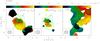 |
Fig. 15 CH3OH(8−1,8 − 70,7), CH3OH (80,8 − 71,6), and C18O(2−1) velocity (1st) moment maps overlaid with the SMA 1.3 mm dust continuum of S255N. The contours start at 5σ and increase in steps of 10σ (1σ = 1.6 mJy beam-1). All moment maps were clipped at the five sigma level of the respective line’s channel map. The lines in each panel show the pv-diagram cut presented in Fig. 14. The synthesized beam is shown in the lower left corner of each plot. The (0, 0) point in each panel is RA 06h12m53.669s Dec + 18°00′26.90′′ (J2000.0). |
3.6.2. SINFONI stellar spectral type classification
Our SINFONI observations provide an H- and K-band spectrum of each source with a spectral resolution of R = 1500. SOFI J- and K-band photometry results are taken from Bik (2004). Objects with K < 14 have high enough S/N spectra to obtain a reliable spectral type. This reduces the sample to 39 sources; however, we can only get the spectral type of 16 sources, which are listed in Table 11. For many point sources, we could not get a spectral type. Some of them have very flat spectra and basically no absorption lines, and also no infrared excess, so they are likely to be gas clumps. Others have very red spectra, which are likely to be dominated by dust emission from the surrounding environment or circumstellar disks; therefore, the spectrum of the underlying objects might not be visible, such as sources #17, #18 in Table 11, and our infrared sources NIRS1 and NIRS3, which are discussed later.
The SINFONI H + K-band spectra of the three brightest cluster members (sources #1, #2, and #3) show Brγ absorption in the K-band and Br10 − 14 absorption in the H-band (Fig. 21). Weaker lines of He I are also visible in H (1.70 μm) and K (2.058 μm). We applied the K-band classification scheme for B stars from Hanson et al. (1996), which links a K-band spectral type to an optical spectral type. For the H-band, we used the classification of Hanson et al. (1998) and Blum et al. (1997). Table 10 shows the measured equivalent widths (EW) of the relevant lines in the H- and K-band spectra of the three B/A stars. Star #1 has a strong Brγ absorption but does not show any He I (2.11 μm), so it is classified as B3V − B7V. Stars #2 and #3 show much stronger Brγ absorption and also do not have He I (2.11 μm), so they are classified as B8V − A3V. The EWs of the H-band lines agree with the K-band spectral type. Sources #1 and #2 are also associated with UCHII regions (Snell & Bally 1986), which suggests that they are high- to intermediate-mass stars, and this is consistent with our spectral type classification results. The results are listed in Table 11.
Besides the 3 B/A stars we found 13 stars showing absorption lines typical with a later spectral type (Fig. 22). The most prominent lines we used are the CO first overtone absorption bands between 2.29 and 2.45 μm, absorption lines of Mg I and other atomic species in the H-band, as well as Ca I and Na I in the K-band. To classify the late-type stars we used the reference spectra of Cushing et al. (2005) and Rayner et al. (2009). The atomic lines, such as Mg I and Na I, are used for the temperature determination, while the CO lines are used to determine the luminosity class. See Bik et al. (2010) for a detailed description.
Compared with the reference spectra, the CO (2.29 μm) absorption of our SINFONI spectra is usually deeper than in dwarf reference spectra, but not as deep as in the giant spectra. In a few cases where a luminosity class IV reference spectrum was available, the spectrum provided a better match to the observed spectrum. This suggests that our late type stars are low- and intermediate PMS stars, and indeed, Luhman (1999) and Winston et al. (2009) find that PMS spectra have a surface gravity midway between giant and dwarf spectra. If the stars were giants, dust veiling could make the K-band CO lines weaker. However, the H-band CO and OH lines are also much weaker, while the atomic lines have the expected EWs. Therefore, this seems to be a surface gravity effect, suggesting a PMS nature for our late type stars.
The “double blind”. procedure was applied during the classification of the late type stars to check the accuracy of the classification. In this procedure, Wang and Bik did their own classification separately and independently without knowing the results of the other, and their results were compared afterwards to get the differences, which are the errors of the spectral type in Table 11. Our classification results showed an error of 1 to 2 subclass in spectral type.
 |
Fig. 16 Position-velocity diagrams derived for the cuts along the observed velocity gradient in Fig. 15. The offset refers to the distance along the cut from the dust continuum peak S255N-SMA1. The contour levels are all from 3σ and in steps of 1σ (1σ = 40 mJy beam-1). |
 |
Fig. 17 CH3CN(12k − 11k) spectrum toward the mm continuum peak S255IR-SMA1. The dotted line shows a model spectrum with Trot = 150 K and NCH3CN = 3.5 × 1014 cm-2. The k = 6 line is excluded in the model because it is blurred by the HNCO(101,9 − 91,8) line. |
 |
Fig. 18 From the Gaussian fitting, we calculated the Nj,k (Zhang et al. 1998) and plotted it in the figure above. Eu is the upper-level energy of each transition. The line shows the linear fitting of the first five points. |
 |
Fig. 19 Three-color image created from SINFONI line maps. Red: Brγ line emission, green: H2 (2.12 μm) line emission and blue: Fe II (1.64 μm) line emission. The cross marks the position of S255IR-SMA1. The contour and the dashed lines mark the regions for which the excitation diagrams are constructed to identify the nature of the emission (Fig. 20). |
 |
Fig. 20 The excitation diagram of the whole arc in the south-east of the Fig. 19 (the top panel) and two jet-like emissions a) and b). The solid line in all diagrams is a single temperature fit to all the lines detected, while for the dash-dotted line in the top panel a only the 1 − 0 S lines are included in the fit. |
The relation from Kenyon & Hartmann (1995) was used to convert the spectral type into effective temperature. However, this relation only applies to main sequence stars, for PMS stars a different relation may hold (Hillenbrand 1997; Winston et al. 2009). Cohen & Kuhi (1979) show that the temperature of PMS stars might be overestimated by values between 500 K (G stars) and 200 K (mid-K). We took this source of error into account when calculating the errors in the effective temperature.
With the knowledge of the spectral type, we can estimate the extinction from the observed color. Since the intrinsic J − K color for dwarfs and giants can differ as much as 0.4 for late K stars (Koornneef 1983), for the PMS stars, we used as the intrinsic J − K color the mean of the color for dwarfs and giants. The difference between the mean value and the dwarf and giant values is used as the error in the intrinsic color. The derived extinctions are listed in Table 11.
3.6.3. YSOs
Sources #17 and #18 have very red spectra and show strong Brγ point emission, but the spectra are featureless due to the strong dust emission, which indicates that they are very young and with ongoing accretion activity (Fig. 23). Source #17 also shows strong K-band CO line emissions (Bik & Thi 2004), which indicates there is a circumstellar disk. The two infrared sources NIRS3 and NIRS1 which coincide with our mm sources S255IR-SMA1 and S255IR-SMA3, respectively, also have extremely red spectra, only several H2 lines can be seen (Fig. 23). Therefore we cannot get the spectral type of these sources.
3.6.4. Cluster membership and the HR diagram
For the late type stars, as discussed in Sect. 3.6.2, most of them have a surface gravity typical of PMS stars, so they are considered to be the cluster members. Sources #15 and #16 show a luminosity type giant and super giant, so they are unlikely to be associated with this young cluster, and since they show quite high extinction, they are considered to be background stars.
Physical properties of the H2 gas.
To constrain the mass of the cluster members and the age of the whole cluster, we construct a HRD to compare the observed parameters with PMS evolutionary tracks. The derived extinctions allow us to de-redden the K-band magnitude, convert to absolute magnitude with the derived temperature, and plot the points in a K vs. log(Teff) diagram (Fig. 25, top). We exclude the background stars #15 and #16 to enable a comparison with the isochrones. The overplotted dashed line is the 2 Myr main sequence isochrone taken from Lejeune & Schaerer (2001). The solid lines in the left panel represent the evolutionary tracks taken from Da Rio et al. (2009) using the models of Siess et al. (2000) for 8 different masses: 5, 4, 3, 2, 1.5, 1, 0.5, 0.4 M⊙. Comparison of the location of the PMS stars with these evolutionary tracks yields an approximate mass varying from ~ 5 M⊙ for the brightest stars to 0.4 M⊙.
Equivalent width and K-band spectral types of the early type stars in S255IR.
Photometric and spectroscopic properties of the detected stars brighter than K = 14 mag.
In the bottom panel of Fig. 25, the overplotted solid lines are the PMS isochrones between 0.1 and 10 Myr. The location of the stars is consistent with a range of age. Except for sources #1, #14, and #4, which lie between the 0.5 and 1 Myr isochrones, most of the objects span the 1 − 3 Myr isochrones, with the more massive objects closer to the 1 Myr isochrone. For the less massive objects, the spread in age is greater, most likely due to higher uncertainties in the spectral type determination. The location of the PMS stars suggests an age of 2 ± 1 Myr.
Comparison of the location of the PMS stars in the HRD with those of the Herbig AeBe stars (van den Ancker et al. 1998) shows that the late spectral type PMS stars are younger than the Herbig AeBe stars and will evolve from their present G- and K spectral type to late B, A, or early F spectral type when they become main sequence stars. The three relatively early spectral type sources (#1, #2, and #3) already evolved to late B early A spectral type. They are in the transit phase between our late spectral type sources and the main sequence.
4. Discussion
4.1. Different evolutionary stages and triggered star formation?
The SMA and IRAM 30 m data together reveal three massive star formation regions with different evolutionary stages. The SCUBA 850 μm image (Fig. 1) presents three continuum peaks in the whole S255 complex region, one in each subregion, which is S255N, S255IR, S255S, from north to south. With our high-resolution SMA observations, ~2500 AU at the given distance of 1.59 kpc, we found that all SCUBA 850 μm sources fragment into several cores.
Minier et al. (2007) suggests that S255S is at a very young stage without active star formation; however, our observations show outflows associated with the mm sources. Furthermore, the virial mass is lower than the mass obtained from the SCUBA 850 μm measurement, which implies that the S255S region will likely collapse. Since the peak column density is also close to or above the proposed threshold for high-mass star formation of 1 g cm-2 (Krumholz & McKee 2008), S255S is at a very early stage of ongoing star formation and may form massive stars. The single-dish continuum properties of S255IR and S255N do not show much difference, but our interferometry and NIR observations show us the different properties of S255IR and S255N. The large-scale NIR emission shows the existence of the NIR cluster in S255IR and not so many NIR point sources in S255N, which indicate S255IR is most likely in a more evolved stage compared to S255N. For the individual subcores, more lines are detected at S255IR-SMA1 than S255N-SMA1, which indicates a higher temperature and the more evolved nature of S255IR-SMA1 compared to S255N-SMA1. Regarding the kinematic properties, S255N-SMA1 has similar outflow velocities but a much smaller size of the outflow than S255IR-SMA1, which may also suggest a younger evolutionary stage of S255N-SMA1. Among other SMA mm continuum cores, S255IR-SMA2, S255N-SMA2, and S255N-SMA3, which do not have many line emissions, are considered to be at earlier evolutionary stages.
 |
Fig. 21 Normalized SINFONI H-band (left panel) and K-band (right panel) spectra of the three B/A stars detected in S255IR. Their spectra are characterized by absorption lines of the hydrogen Bracket series and He I (dotted vertical lines). The stars are numbered according to Table 11. |
Figure 1 presents the whole star formation region. The young star formation region S255 complex lies between the evolved H II regions, S255 and S257. From the morphology of the dust structure and the H II regions, it appears that the two H II regions pushed gas between them, formed the S255IR dust structure, and triggered the star formation, which has also been suggested by Bieging et al. (2009) and Minier et al. (2007). To inquire into that, we studied the velocity map of our 30 m data; however, due to the high noise level at the edge of the map, we could not find a significant velocity difference between the western and eastern edges of the dust structure to prove the interaction between the H II regions and the dust structure. Chavarría et al. (2008) estimated the dynamical age of the two H II regions S255 and S257, which is ~1.5 × 10⁶ yr, similar to our NIR cluster in S255IR. So we can not prove the triggering star formation. However, we witness outflow interaction between S255IR and S255N (Sect. 3.3). Since S255N is younger than S255IR, S255N may be affected by S255IR.
Furthermore, the age of the cluster we obtained around S255IR from the SINFONI data is 2 ± 1 Myr (Sect. 3.6.4). Chavarría et al. (2008) obtained an age of the larger scale cluster of 1 Myr which is consistent with our result. However, the dynamical age of the high-mass protostar in this region, S255IR-SMA1, is ~104 yr (Table 8). Without the knowledge of the outflow inclination angle, we could systematically underestimate the age value by a factor of 2 to 5 (Cabrit & Bertout 1992). Therefore, S255IR-SMA1 should not be dynamically older than 105 yr and S255IR-SMA2 is even younger than S255IR-SMA1. The age difference between the NIR cluster and the massive protostellar objects indicates that the most massive sources in the cluster form last.
Minier et al. (2007) suggests a collect-and-collapse and triggered star formation scenario for S255IR, which is that the B-stars (from our observations they are late B stars, i.e. stars #1, #2, #3 in Fig. 24) in S255IR formed through a collect-and-collapse process, and triggered the formation of NIRS 1 and NIRS 3. The NIR and mm data presented in this paper show that the cluster detected in the infrared is likely older than the mm sources detected with our SMA data. While the SMA mm sources lie in the center of the NIR cluster, the NIR cluster members are more distributed around the mm sources. Based on this information, we propose an outside-in star formation scenario, which is that the central gas filament collapses under the pressure of the two H II regions. The collapse of the clump may start outside-in under the pressure of the two H II regions, the low-mass cores need lower density to form, and they formed first in the outside region of the clump and collapse to stars. And then either the low- to intermediate-mass stars may enhance the instability of the central high-mass cores and potentially trigger the high-mass star formation in S255IR, or the massive cores could build up slightly more slowly and start to collapse afterwards, forming the most massive stars in this region. Our outflow observations hint that the energetic outflow from the YSOs in S255IR may have again affected the star formation in S255N, but this needs further observations to confirm.
However, the different evolutionary stages of the various regions, even within each region are quite clear. This suggests a sequential star formation.
4.2. Multiple outflows
We detected outflows in all three regions (Sect. 3.3). In the top panels of Fig. 8, the outflow emission that is close to the SMA continuum sources does not really follow the NE-SW direction. We suggest this complicated outflow environment in the nearby region of the continuum sources comes from the interaction between outflows from NIRS 1 and NIRS 3. The red-shifted lobe to the S of the continuum source (bottom panels in Fig. 8) is most likely driven by NIRS 1, because the N-S bipolar reflection nebular associated with NIRS 1 follows this direction to the S (Jiang et al. 2008; Simpson et al. 2009), and the outflow driven by NIRS 3 should be blue-shifted at this direction.
 |
Fig. 22 Normalized SINFONI H-band (left panel) and K-band (right panel) spectra of the 11 objects showing late-type stellar spectral type. And most of them are PMS stars. The vertical lines show the location of some of the absorption lines used for the classification of the stars. The stars are numbered according to Table 11. |
In Fig. 10, the red-shifted gas at the bottom part of line (b) seems to be associated with S255N-SMA3; however, another blue-shifted feature in the southern part of the map shows up as the resolution changes. Figure 7 shows that these components are mixed with the outflows in S255IR, which may indicate the interaction between these two regions.
In the youngest region S255S, the velocity of the outflows is much smaller than the other two regions. Table 2 shows that the column density of this region is still relatively low, S255S is in a very young evolutionary stage and likely to just start collapsing. This is the reason we did not detect any very energetic outflows like for the other two regions in this region.
 |
Fig. 23 SINFONI H-band (left panel) and K-band (right panel) spectra of the 4 YSOs. The stars are numbered as in Table 11. |
 |
Fig. 24 The stars listed in Table 11 marked on the Brγ line + continuum map overlaid with H2 line emission contours. |
 |
Fig. 25 Top: the extinction corrected K vs. log(Teff) HRD. The K-band magnitude has been corrected for the distance modulus. Overplotted with a dashed line is the 2 Myr main sequence isochrone from Lejeune & Schaerer (2001), and with the solid lines the pre-main-sequence evolutionary tracks from Da Rio et al. (2009). Bottom: the same data but overplotted with solid lines showing the isochrones from Da Rio et al. (2009). |
4.3. Disk candidates in S255IR
NIRS 1, which coincides with S255IR-SMA3, is reported to have a polarization disk (Jiang et al. 2008). Simpson et al. (2009) also report a disk, but one with a slightly different interpretation. Because NIRS 1 is relatively more evolved, we detected only one unresolved mm continuum source associated with only the CO isotopologue lines (Sect. 3.2). NIRS 3, which coincides with S255IR-SMA1, is considered to be a high-mass protostar based on several signatures (e.g., UCHII region, maser emissions, hot core emissions, and energetic outflows, see Sects. 1 and 3). We detected a rotational structure coinciding with this source perpendicular to the outflow (Fig. 13). The HCOOCH3 position velocity diagram shows that this rotational structure is not Keplerian, so it could be a rotating toroid around NIRS 3. However, the C18O pv-diagram shows a much larger Keplerian-like velocity structure perpendicular to the outflow (Fig. 14). If this source were much farther away or observed with worse resolution, this structure could be easily identified as a disk. However, with our resolution we resolved two mm source, so we know it is not a disk. The C18O gas size is ~2 × 10⁴ AU and the continuum source has a size of 1.6 × 10⁴ AU at the given distance of 1.59 × 10³ pc, which is similar to the rotational structure described in Fallscheer et al. (2009). This structure is also much larger than the jeans length, which is ~6000 AU for a temperature ~20 K and a density ~1 × 10⁶. Our system also exceeds the criteria to maintain a stable disk described by Kratter et al. (2010). Therefore, we suggest that this structure is a rotating toroid that fragmented into several sources to formed a multiple system. Similar structures of fragmenting pseudo-disks have also been modeled by Krumholz et al. (2009) and Peters et al. (2010).
Following these, we propose a star formation scenario for this large rotational structure, which is that the rotational elongated dust structure formed first, and the massive source NIRS 1 started forming in the central region. However, this large structure is much more massive than NIRS 1 and is unstable, and then it fragmented into two sources, S255IR-SMA1 and S255IR-SMA2.
The SINFONI source #17 shows strong Brγ and CO emission in K-band (Fig. 23), which indicates there is a circumstellar disk. Source #17 might also drive the jet-like emissions at the northern edge of Fig. 19. It is interesting to find disk signatures toward sources with these different evolutionary stages within the same forming cluster.
4.4. Cores and clumps
Since the single dish has a much larger beam, which can cover all the continuum sources, and 13CO may be optically thick, the observed velocity traces the outer layer of the whole clump and shows the mean line-of-sight velocity. The molecular lines we used to get the velocities for the SMA observations are all dense gas and disk tracers (Cesaroni et al. 2007), so what we obtained are the velocities of the high-mass cores (Table 6). The difference between the core velocities and the clump velocities of several km s-1 (Table 6) are very different from the low-mass core cases (e.g. 0.46 km s-1 in NGC 1336 Walsh et al. 2007; 0.17 km s-1 in Oph A Di Francesco et al. 2004). This difference confirms that massive star formation regions are more turbulent than low-mass ones. It further implies stronger peculiar motions of the protostars and cores within the clump/cluster gravitational potential.
5. Summary
Combining multiwavelength data from mm to NIR wavelength, we characterized the different (proto) stellar populations within the S255 star formation complex. S255S, S255N, and S255IR show different dynamical and chemical properties, not only at mm wavelength but also at infrared wavelengths, which indicates they are in different evolutionary stages. With the SMA, IRAM 30 m, and VLT-SINFONI observations, we found outflows in all three regions, high-velocity collimated ones in S255IR, high-velocity more confined ones in S255N, and lower velocity confined ones in S255S. The multiple outflows we found in S255IR and S255N suggests a potential interaction between these two regions. From the outflow maps, we estimated the dynamical age of the outflow driving sources. Although without the information of the inclination angle, this dynamical age could be underestimated by a factor of 2 to 5 (Cabrit & Bertout 1992), our mm sources should not be older than 105 yr.
We detected 25 molecular lines in S255IR, including 7 lines of the CH3CN(12k − 11k) k-ladder with k = 0...6, confirming the hot core nature of S255IR-SMA1. Only 10 molecular lines are detected in S255N, including 2 CH3CN(12k − 11k) k-ladder with k = 0, 1, which is indicative of a younger age and colder temperature. Besides the 3 CO isotopologue line emissions, only diffuse SO emission is detected in S255S. This is consistent with different chemical ages.
High-density tracers like CH3CN and HCOOCH3 show rotational structures around the most prominent high-mass protostar candidates in S255IR and S255N. Furthermore in S255IR, the C18O presents an elongated rotational structure with a Keplerian-like velocity gradient perpendicular to the outflow. With a size of ~2 × 10⁴ AU, this structure cannot be a disk but may be a rotational toroid that fragments into several sources.
Near infrared H- and K-band integral field spectroscopy observations were done for S255IR. We identified the excitation mechanism of the H2 emission. We derived the spectral type of 16 stars, and 14 of them are considered to be the cluster members. With the knowledge of the spectral type and the SOFI J- and K-band photometry results (Bik 2004) of the cluster members, we constructed an HR diagram to estimate the age of the cluster, which is 2 ± 1 Myr . This age is consistent with the result Chavarría et al. (2008) obtained. The age difference between the low-mass cluster and the massive mm cores indicates different stellar populations in the cluster. This also leads to a question, do the massive stars in this cluster form last? Our data support the idea that massive stars form last. We propose the triggered outside-in collapse star formation scenario for the bigger picture and the fragmentation scenario for S255IR
The whole picture of the S255 complex suggests triggered star formation, however, but we cannot give hard proof at present. However, the different evolutionary stages between each region and different stellar populations in S255IR are consistent with sequential star formation.
The MIR cookbook by Chunhua Qi can be found at http://cfa-www.harvard.edu/~cqi/mircook.html.
Acknowledgments
The authors thank C. J. Cyganowski for providing the VLA 3.6 cm data of S255N, F. Eisenhauer for providing the data reduction software SPRED, A. Modigliani for help in the data reduction, R. Davies for providing his routines for removing the OH line residuals, N. Da Rio for providing the isochrones and evolutionary tracks, M. Fang and A. Sobolev for the discussion.
Y.W. acknowledges support by Purple Mountain Observatory, CAS and Max-Plank-Institute for Astronomy. E.P. is funded by the Spanish MICINN under the Consolider-Ingenio 2010 Program grant CSD2006-00070: First Science with the GTC.
References
- Abuter, R., Schreiber, J., Eisenhauer, F., et al. 2006, New Astron. Rev., 50, 398 [NASA ADS] [CrossRef] [Google Scholar]
- Arce, H. G., Shepherd, D., Gueth, F., et al. 2007, in Protostars and Planets V, ed. B. Reipurth, D. Jewitt, & K. Keil (Tucson: Univ. Arizona Press), 245 [Google Scholar]
- Beuther, H., Schilke, P., Sridharan, T. K., et al. 2002, A&A, 383, 892 [NASA ADS] [CrossRef] [EDP Sciences] [Google Scholar]
- Beuther, H., Schilke, P., Menten, K. M., et al. 2005a, ApJ, 633, 535 [NASA ADS] [CrossRef] [Google Scholar]
- Beuther, H., Zhang, Q., Greenhill, L. J., et al. 2005b, ApJ, 632, 355 [NASA ADS] [CrossRef] [Google Scholar]
- Beuther, H., Zhang, Q., Bergin, E. A., & Sridharan, T. K. 2009, AJ, 137, 406 [NASA ADS] [CrossRef] [Google Scholar]
- Bieging, J. H., Peters, W. L., Vi la Vilaro, B., Schlottman, K., & Kulesa, C. 2009, AJ, 138, 975 [NASA ADS] [CrossRef] [Google Scholar]
- Bik, A. 2004, Ph.D. Thesis [Google Scholar]
- Bik, A., & Thi, W. F. 2004, A&A, 427, L13 [NASA ADS] [CrossRef] [EDP Sciences] [Google Scholar]
- Bik, A., Puga, E., Waters, L. B. F. M., et al. 2010, ApJ, 713, 883 [NASA ADS] [CrossRef] [Google Scholar]
- Blum, R. D., Ramond, T. M., Conti, P. S., Figer, D. F., & Sellgren, K. 1997, AJ, 113, 1855 [NASA ADS] [CrossRef] [Google Scholar]
- Bonnet, H., Abuter, R., Baker, A., et al. 2004, The Messenger, 117, 17 [NASA ADS] [Google Scholar]
- Cabrit, S., & Bertout, C. 1990, ApJ, 348, 530 [NASA ADS] [CrossRef] [Google Scholar]
- Cabrit, S., & Bertout, C. 1992, A&A, 261, 274 [Google Scholar]
- Cesaroni, R., Galli, D., Lodato, G., Walmsley, C. M., & Zhang, Q. 2007, Protostars and Planets V, 197 [Google Scholar]
- Chavarría, L. A., Allen, L. E., Hora, J. L., Brunt, C. M., & Fazio, G. G. 2008, ApJ, 682, 445 [NASA ADS] [CrossRef] [Google Scholar]
- Choi, M., Evans, II, N. J., & Jaffe, D. T. 1993, ApJ, 417, 624 [NASA ADS] [CrossRef] [Google Scholar]
- Cohen, M., & Kuhi, L. V. 1979, ApJS, 41, 743 [NASA ADS] [CrossRef] [Google Scholar]
- Cohen, M., Wheaton, W. A., & Megeath, S. T. 2003, AJ, 126, 1090 [NASA ADS] [CrossRef] [Google Scholar]
- Cushing, M. C., Rayner, J. T., & Vacca, W. D. 2005, ApJ, 623, 1115 [NASA ADS] [CrossRef] [Google Scholar]
- Cyganowski, C. J., Brogan, C. L., & Hunter, T. R. 2007, AJ, 134, 346 [NASA ADS] [CrossRef] [Google Scholar]
- Da Rio, N., Gouliermis, D. A., & Henning, T. 2009, ApJ, 696, 528 [NASA ADS] [CrossRef] [Google Scholar]
- Davies, R. I. 2007, MNRAS, 375, 1099 [NASA ADS] [CrossRef] [Google Scholar]
- Davis, C. J., Smith, M. D., Stern, L., Kerr, T. H., & Chiar, J. E. 2003, MNRAS, 344, 262 [NASA ADS] [CrossRef] [Google Scholar]
- Di Francesco, J., André, P., & Myers, P. C. 2004, ApJ, 617, 425 [NASA ADS] [CrossRef] [Google Scholar]
- Di Francesco, J., Johnstone, D., Kirk, H., MacKenzie, T., & Ledwosinska, E. 2008, ApJS, 175, 277 [NASA ADS] [CrossRef] [Google Scholar]
- Eisenhauer, F., Abuter, R., Bickert, K., et al. 2003, in SPIE Conf. Ser. 4841, ed. M. Iye, & A. F. M. Moorwood, 1548 [Google Scholar]
- Fallscheer, C., Beuther, H., Zhang, Q., Keto, E., & Sridharan, T. K. 2009, A&A, 504, 127 [NASA ADS] [CrossRef] [EDP Sciences] [Google Scholar]
- Goddi, C., Moscadelli, L., Sanna, A., Cesaroni, R., & Minier, V. 2007, A&A, 461, 1027 [NASA ADS] [CrossRef] [EDP Sciences] [Google Scholar]
- Goldsmith, P. F., Langer, W. D., & Velusamy, T. 1999, ApJ, 519, L173 [NASA ADS] [CrossRef] [Google Scholar]
- Hanson, M. M., Conti, P. S., & Rieke, M. J. 1996, ApJS, 107, 281 [Google Scholar]
- Hanson, M. M., Rieke, G. H., & Luhman, K. L. 1998, AJ, 116, 1915 [NASA ADS] [CrossRef] [Google Scholar]
- Hildebrand, R. H. 1983, QJRAS, 24, 267 [NASA ADS] [Google Scholar]
- Hillenbrand, L. A. 1997, AJ, 113, 1733 [NASA ADS] [CrossRef] [Google Scholar]
- Hollenbach, D., & McKee, C. F. 1989, ApJ, 342, 306 [NASA ADS] [CrossRef] [Google Scholar]
- Jiang, Z., Tamura, M., Hoare, M. G., et al. 2008, ApJ, 673, L175 [NASA ADS] [CrossRef] [Google Scholar]
- Jørgensen, J. K., Hogerheijde, M. R., Blake, G. A., et al. 2004, A&A, 415, 1021 [NASA ADS] [CrossRef] [EDP Sciences] [Google Scholar]
- Kalenskii, S. V., Slysh, V. I., & Val’tts, I. E. 2002, in Cosmic Masers: From Proto-Stars to Black Holes, ed. V. Migenes, & M. J. Reid, IAU Symp. 206, 191 [Google Scholar]
- Kenyon, S. J., & Hartmann, L. 1995, ApJS, 101, 117 [NASA ADS] [CrossRef] [Google Scholar]
- Klein, R., Posselt, B., Schreyer, K., Forbrich, J., & Henning, T. 2005, ApJS, 161, 361 [NASA ADS] [CrossRef] [Google Scholar]
- Koornneef, J. 1983, A&A, 128, 84 [NASA ADS] [Google Scholar]
- Kratter, K. M., Matzner, C. D., Krumholz, M. R., & Klein, R. I. 2010, ApJ, 708, 1585 [NASA ADS] [CrossRef] [Google Scholar]
- Krumholz, M. R., & McKee, C. F. 2008, Nature, 451, 1082 [NASA ADS] [CrossRef] [PubMed] [Google Scholar]
- Krumholz, M. R., Klein, R. I., McKee, C. F., Offner, S. S. R., & Cunningham, A. J. 2009, Science, 323, 754 [NASA ADS] [CrossRef] [PubMed] [Google Scholar]
- Kurtz, S., Churchwell, E., & Wood, D. O. S. 1994, ApJS, 91, 659 [NASA ADS] [CrossRef] [Google Scholar]
- Kurtz, S., Hofner, P., & Álvarez, C. V. 2004, ApJS, 155, 149 [NASA ADS] [CrossRef] [Google Scholar]
- Lejeune, T., & Schaerer, D. 2001, A&A, 366, 538 [NASA ADS] [CrossRef] [EDP Sciences] [Google Scholar]
- Levreault, R. M. 1988, ApJ, 330, 897 [NASA ADS] [CrossRef] [Google Scholar]
- Longmore, S. N., Burton, M. G., Minier, V., & Walsh, A. J. 2006, MNRAS, 369, 1196 [NASA ADS] [CrossRef] [Google Scholar]
- Luhman, K. L. 1999, ApJ, 525, 466 [NASA ADS] [CrossRef] [Google Scholar]
- Martín-Hernández, N. L., Bik, A., Puga, E., Nürnberger, D. E. A., & Bronfman, L. 2008, A&A, 489, 229 [NASA ADS] [CrossRef] [EDP Sciences] [Google Scholar]
- Minier, V., Booth, R. S., & Conway, J. E. 2000, A&A, 362, 1093 [NASA ADS] [Google Scholar]
- Minier, V., Burton, M. G., Hill, T., et al. 2005, A&A, 429, 945 [NASA ADS] [CrossRef] [EDP Sciences] [Google Scholar]
- Minier, V., Peretto, N., Longmore, S. N., et al. 2007, in IAU Symp. 237, ed. B. G. Elmegreen, & J. Palous, 160 [Google Scholar]
- Miralles, M. P., Salas, L., Cruz-Gonzalez, I., & Kurtz, S. 1997, ApJ, 488, 749 [Google Scholar]
- Müller, H. S. P., Thorwirth, S., Roth, D. A., & Winnewisser, G. 2001, A&A, 370, L49 [NASA ADS] [CrossRef] [EDP Sciences] [Google Scholar]
- Muzerolle, J., Hartmann, L., & Calvet, N. 1998, AJ, 116, 2965 [NASA ADS] [CrossRef] [Google Scholar]
- Nomura, H., & Millar, T. J. 2004, A&A, 414, 409 [NASA ADS] [CrossRef] [EDP Sciences] [MathSciNet] [Google Scholar]
- Ojha, D., Tamura, M., & Sirius Team. 2006, Bull. Astron. Soc. Ind., 34, 119 [Google Scholar]
- Ossenkopf, V., & Henning, T. 1994, A&A, 291, 943 [NASA ADS] [Google Scholar]
- Peters, T., Klessen, R. S., Mac Low, M., & Banerjee, R. 2010, ApJ, 725, 134 [NASA ADS] [CrossRef] [Google Scholar]
- Poynter, R. L., & Pickett, H. M. 1985, Appl. Opt., 24, 2235 [NASA ADS] [CrossRef] [PubMed] [Google Scholar]
- Rayner, J. T., Cushing, M. C., & Vacca, W. D. 2009, ApJS, 185, 289 [NASA ADS] [CrossRef] [Google Scholar]
- Rygl, K. L. J., Brunthaler, A., Reid, M. J., et al. 2010, A&A, 511, A2 [NASA ADS] [CrossRef] [EDP Sciences] [Google Scholar]
- Sault, R. J., Teuben, P. J., & Wright, M. C. H. 1995, in Astronomical Data Analysis Software and Systems IV, ed. R. A. Shaw, H. E. Payne, & J. J. E. Hayes, ASP Conf. Ser., 77, 433 [Google Scholar]
- Schreiber, J., Thatte, N., Eisenhauer, F., et al. 2004, in Astronomical Data Analysis Software and Systems (ADASS) XIII, ed. F. Ochsenbein, M. G. Allen, & D. Egret, ASP Conf. Ser., 314, 380 [Google Scholar]
- Scoville, N. Z., Carlstrom, J. E., Chandler, C. J., et al. 1993, PASP, 105, 1482 [NASA ADS] [CrossRef] [Google Scholar]
- Siess, L., Dufour, E., & Forestini, M. 2000, A&A, 358, 593 [NASA ADS] [Google Scholar]
- Simpson, J. P., Burton, M. G., Colgan, S. W. J., et al. 2009, ApJ, 700, 1488 [NASA ADS] [CrossRef] [Google Scholar]
- Slysh, V. I., Kalenskiĭ, S. V., & Val’tts, I. E. 2002, Astron. Rep., 46, 49 [Google Scholar]
- Snell, R. L., & Bally, J. 1986, ApJ, 303, 683 [NASA ADS] [CrossRef] [Google Scholar]
- Sobolev, A. M., Sutton, E. C., Cragg, D. M., & Godfrey, P. D. 2005, Ap&SS, 295, 189 [NASA ADS] [CrossRef] [Google Scholar]
- Sobolev, A. M., Cragg, D. M., Ellingsen, S. P., et al. 2007, in IAU Symp. 242, ed. J. M. Chapman, & W. A. Baan, 81 [Google Scholar]
- Sutton, E. C., Blake, G. A., Masson, C. R., & Phillips, T. G. 1985, ApJS, 58, 341 [NASA ADS] [CrossRef] [Google Scholar]
- Sutton, E. C., Sobolev, A. M., Salii, S. V., et al. 2004, ApJ, 609, 231 [NASA ADS] [CrossRef] [Google Scholar]
- Tamura, M., Gatley, I., Joyce, R. R., et al. 1991, ApJ, 378, 611 [NASA ADS] [CrossRef] [Google Scholar]
- van den Ancker, M. E., de Winter, D., & Tjin A Djie, H. R. E. 1998, A&A, 330, 145 [NASA ADS] [Google Scholar]
- Walsh, A. J., Myers, P. C., Di Francesco, J., et al. 2007, ApJ, 655, 958 [NASA ADS] [CrossRef] [Google Scholar]
- Winston, E., Megeath, S. T., Wolk, S. J., et al. 2009, AJ, 137, 4777 [NASA ADS] [CrossRef] [Google Scholar]
- Xu, Y., Voronkov, M. A., Pandian, J. D., et al. 2009, A&A, 507, 1117 [NASA ADS] [CrossRef] [EDP Sciences] [Google Scholar]
- Zhang, Q., Ho, P. T. P., & Ohashi, N. 1998, ApJ, 494, 636 [NASA ADS] [CrossRef] [Google Scholar]
All Tables
Photometric and spectroscopic properties of the detected stars brighter than K = 14 mag.
All Figures
|
Fig. 1 SPITZER IRAC 4.5 μm image (Chavarría et al. 2008) overlaid with SCUBA 850 μm contours (Di Francesco et al. 2008; Klein et al. 2005). In the upper panel, the gray scale is the SPITZER IRAC 4.5 μm image, the black contours are the NVSS 1.4 GHz emission and the green contours are the SCUBA 850 μm continuum. In the bottom left panel, the gray scale is the SPITZER MIPS 24 μm image, the contours are the SCUBA 850 μm continuum, the three dashed circles mark the primary beam of our SMA observations. In the bottom right panel, the gray scale is the SPITZER MIPS 70 μm image, the contours and the circles are the same as the ones in the left panel. The contour levels of the NVSS start at 10σ (1σ = 0.6 mJy beam-1) in steps of 5σ. For the SCUBA 850 μm, the contour levels start at 10σ (1σ = 0.1 Jy beam-1) with a step of 10σ. The SPITZER/IRAC post-bcd data processed with pipeline version S18.7.0 and the MIPS post-bcd data processed with pipeline version S17.2.0 have been downloaded from the SPITZER archive to create these images. |
| In the text | |
|
Fig. 2 Lower and upper sideband spectral vector-averaged over all baselines with a resolution of 2 km s-1 per channel. In the upper sideband image, the 12CO line in S255IR and S255N panels was not fully plotted, which goes to 11.6 Jy and 5.9 Jy, respectively. |
| In the text | |
|
Fig. 3 The SMA 1.3 mm continuum map of S255IR, S255N, and S255S. contour levels start at 5σ in steps of 5σ in S255IR (1σ = 1.7 mJy/beam) and S255N (1σ = 1.6 mJy/beam) image and 3σ in S255S (1σ = 0.9 mJy/beam) image. The dotted contours are the negative features due to the missing flux. The synthesis beam is shown at the bottom left of each figure. In the S255IR panel, the asterisk marks the position of NIRS 3 and the right one marks NIRS 1 (Tamura et al. 1991). The inset is a zoom in the continuum image of the inner region of S255IR-SMA1 and the contour levels start at 5σ in steps of 10σ. The triangles are the water masers (Goddi et al. 2007) and the two open diamond mark the positions of two 6.7 GHz methanol masers detected by Xu et al. (2009). In S255N panel, the crosses mark the position of the Class I 44 GHz (70 − 61) A+ methanol masers detected by Kurtz et al. (2004) and the triangle is the water maser (Cyganowski et al. 2007). The (0, 0) point in each panel from left to right is RA 06h12m54.019s Dec 17°59′23.10′′ (J2000.0), RA 06h12m53.669s Dec + 18°00′26.90′′ (J2000.0) and RA 06h12m56.58s Dec + 17°58′32.80′′ (J2000.0), respectively. |
| In the text | |
|
Fig. 4 S255IR CH3OH line integrated intensity images with the SMA 1.3 mm continuum emission in the background. Contour levels start at 3σ with 2σ/level. For the top panels, the σ of the contours in each panel, from left to right, is 12, 15, 11 mJy beam-1, respectively, and for the bottom panels is 12, 14, 15 mJy beam-1, respectively. The dotted contours are the negative feature. The integral velocity ranges are shown in the bottom left corner of each panel in km s-1. The synthesized beams are shown in the bottom left corner of each panel. The (0, 0) point in each panel is RA 06h12m54.019s Dec + 17°59′23.10′′ (J2000.0). |
| In the text | |
|
Fig. 5 S255IR molecular line integrated intensity contour with the SMA 1.3 mm continuum emission in the background. All the contour levels start at 3σ. The contour step is 3σ in SO (1σ = 22 mJy beam-1), HCOOH (1σ = 10 mJy beam-1), HCOOCH3 (1σ = 12 mJy beam-1), C18O (1σ = 16 mJy beam-1), CH3CN (1σ = 11 mJy beam-1) and HNCO (1σ = 13 mJy beam-1) images, and 1σ in OCS (1σ = 13 mJy beam-1) and 13CS (1σ = 11 mJy beam-1) image. The dotted contours are the negative features with the same contours as the positive ones in each panel. The integral velocity ranges are shown in the bottom left corner of each panel in km s-1. The synthesized beams are shown in the bottom left corner of each panel. We only plotted the line for CH3CN and (100,10 − 90,9) line for HNCO. The (0, 0) point in each panel is RA 06h12m54.019s Dec + 17°59′23.10′′ (J2000.0). |
| In the text | |
|
Fig. 6 S255N molecular line integrated intensity contour with the SMA 1.3 mm continuum emission in the background. All the contour levels start at 3σ. The contour step is 1σ in CH3OH(80,8 − 71,6)A- (1σ = 9 mJy beam-1) and CH3CN(, 1σ = 14 mJy beam-1) images, 2σ in 13CS (1σ = 25 mJy beam-1) image, 3σ in SO (1σ = 13 mJy beam-1) and CH3OH(81,8 − 70,7)E images, and 0.5σ in OCS (1σ = 10 mJy beam-1) image. The dotted contours are the negative features. The integral velocity ranges are shown in the bottom-left corner of each panel in km s-1. The synthesized beams are shown in the bottom left of each panel. The (0, 0) point in each panel is RA 06h12m53.669s Dec + 18°00′26.90′′ (J2000.0). |
| In the text | |
|
Fig. 7 The single-dish outflow map of the S255 complex. The blue-shifted outflow is shown in dashed contours with a velocity-integration regime of [−40, 0] km s-1, and the red one is shown in full contours with a velocity-integration regime of [16, 56] km s-1. The contours start at 4σ in steps of 5σ (1σ = 1.2 K km s-1). The three crosses mark the position of the three SCUBA 850 μm continuum sources. |
| In the text | |
|
Fig. 8 S255IR 12CO(2−1) outflow images observed with IRAM 30 m telescope and the SMA. The blue-shifted outflow is shown in dashed contours with a velocity-integration regime of [−40, 0] km s-1, and the red one is shown in full contours with a velocity-integration regime of [16, 56] km s-1. The top left panel presents the SMA data only map, the bottom right one presents the IRAM 30 m data only map. The others are all combined SMA + 30 m data, which are inverted with different uv-range selections (shown in the top right of each panel in kλ) resulting in different beam sizes shown in the bottom left corner of each panel. All the 12CO emission contour levels start at 5σ in steps of 10σ. The dotted contours are the negative features and the stars mark the position of NIRS 3. In the bottom left panel, the background scale is SINFONI H2 line emission. The line in the SMA-only panel shows the pv-cut presented in Fig. 9, and the cross marks the central position of the line. In panel (0, 120), the SMA 1.3 mm continuum map is overplotted (black full contours), and the contours start at 5σ in steps of 5σ. In panel (0, 70), the same CH3OH (8−1,8 − 70,7)E integrated intensity map in Fig. 4 is over plotted in black full contours . The σ of the outflow data is shown in Table 7. The (0, 0) point in each panel is RA 06h12m54.019s Dec + 17°59′23.10′′ (J2000.0). |
| In the text | |
|
Fig. 9 Position-velocity diagrams of S255IR for the 12CO(2 − 1) SMA-only outflow observations with a velocity resolution of 1 km s-1. The pv-diagram is in NE-SW direction with a PA of 75° from the N (the cut is marked in Fig. 8, top-left panel). The contour levels are from 10 to 90% from the peak emission (4.2 Jy beam-1) in steps of 10%. The vlsr at 7.7 km s-1 and the central position (marked by the cross in Fig. 8top-left panel) are marked by vertical and horizontal lines. |
| In the text | |
|
Fig. 10 S255N 12CO(2−1) outflow images observed with IRAM 30 m telescope and the SMA. The blue-shifted outflow is shown in dashed contours with a velocity-integration regime of [−44, 0] km s-1, and the red one is shown in full contours with a velocity-integration regime of [16, 48] km s-1. The left panel presents the SMA data only map, the right presents the IRAM 30 m data only map. The synthesized beam is shown in the bottom left corner of each panel. The middle one is combined SMA + 30 m data, the uv-range selection is shown in the top right of each panel in kλ. All the CO emission contour levels start at 5σ in steps of 6σ. The dotted contours are the negative features and the asterisks mark the position of continuum peaks. In the middle panel, the crosses mark the position of the Class I 44 GHz (70 − 61) A+ methanol masers detected by Kurtz et al. (2004) and the triangle is the water maser (Cyganowski et al. 2007). In the top left panel, the background gray scale is VLA Q-band continuum (Cyganowski et al. 2007) and the line shows the pv-cut presented in Fig. 11, which follows the masers direction and crosses the continuum peak. The arrow in the 30 m-only panel marks the outflow size we used to calculate the outflow physical parameters. The σ of the outflow data is shown in Table 7. The (0, 0) point in each panel is RA 06h12m53.669s Dec + 18°00′26.90′′ (J2000.0). |
| In the text | |
|
Fig. 11 Position-velocity diagrams of S255N for the 12CO(2 − 1) SMA-only outflow observations with a velocity resolution of 1 km s-1. The top panel is the pv-plot in NE-SW direction with a PA of 54° from the N (the cut is marked as the line a in Fig. 10, left panel), and the bottom panel is the pv-plot in NW-SE direction with a PA of 7° from the N. (The cut is marked as the line b in Fig. 10, left panel.) The contour levels are from 10 to 90% from the peak emission (4.15 Jy beam-1 in the top panel and 2.82 Jy beam-1 in the bottom panel) in steps of 10%. The vlsr at 8.6 km s-1 and the central position (i.e. the S255N-SMA1 position in the top panel and the cross point of lines a and b in Fig. 10 top-left panel in the bottom panel) are marked by horizontal and vertical lines. |
| In the text | |
|
Fig. 12 S255S 12CO(2 − 1) outflow images observed with IRAM 30 m telescope and the SMA. The blue-shifted outflow is shown in dashed contours with a velocity-integration regime of [−9, 1] km s-1, and the red one is shown in full contours with a velocity-integration regime of [14, 32] km s-1. The left panel presents the SMA data only map, the right presents the IRAM 30 m data only map. The synthesized beam is shown in the bottom left corner of each panel. The middle one is combined SMA + 30 m data, and the uv-range selection is shown in the top right of each panel in kλ. All the 12CO(2 − 1) emission contour levels start at 5σ in steps of 4σ, except the one in the IRAM 30 m only image, which starts at 5σ in steps of 2σ. The dotted contours are the negative features and the stars mark the positions of continuum peak S255S-SMA1 and S255S-SMA2. The arrows in the 30 m-only panel mark the outflow sizes we used to calculate the outflow physical parameters. The σ of the outflow data is shown in Table 7. The (0, 0) point in each panel corresponds to position RA 06h12m56.58s Dec + 17°58′32.80′′ (J2000.0). |
| In the text | |
|
Fig. 13 HCOOCH3, CH3CN (k = 2), and C18O(2−1) velocity (1st) moment maps overlaid with the SMA 1.3 mm dust continuum of S255IR. The contours start at 5σ and increase in steps of 10σ in all panels (σ = 1.7 mJy beam-1). The lines in each panel show the pv-diagram cut presented in Fig. 14. All moment maps were clipped at the five sigma level of the respective line channel map. The synthesized beam is shown in the bottom left corner of each plot. The (0, 0) point in each panel is RA 06h12m54.019s Dec + 17°59′23.10′′ (J2000.0). |
| In the text | |
|
Fig. 14 Position-velocity diagrams derived for the cuts along the observed velocity gradient in Fig. 13. The offset refers to the distance along the cut from the dust continuum peak. The contour levels are from 3σ in steps of 1σ in both panels (1σ = 60 mJy beam-1). The full line in the C18O panel shows a Keplerian rotation curve with a central mass of 28 M⊙, which is the mass of the whole continuum structure in S255IR. The negative features are shown by dashed lines. |
| In the text | |
|
Fig. 15 CH3OH(8−1,8 − 70,7), CH3OH (80,8 − 71,6), and C18O(2−1) velocity (1st) moment maps overlaid with the SMA 1.3 mm dust continuum of S255N. The contours start at 5σ and increase in steps of 10σ (1σ = 1.6 mJy beam-1). All moment maps were clipped at the five sigma level of the respective line’s channel map. The lines in each panel show the pv-diagram cut presented in Fig. 14. The synthesized beam is shown in the lower left corner of each plot. The (0, 0) point in each panel is RA 06h12m53.669s Dec + 18°00′26.90′′ (J2000.0). |
| In the text | |
|
Fig. 16 Position-velocity diagrams derived for the cuts along the observed velocity gradient in Fig. 15. The offset refers to the distance along the cut from the dust continuum peak S255N-SMA1. The contour levels are all from 3σ and in steps of 1σ (1σ = 40 mJy beam-1). |
| In the text | |
|
Fig. 17 CH3CN(12k − 11k) spectrum toward the mm continuum peak S255IR-SMA1. The dotted line shows a model spectrum with Trot = 150 K and NCH3CN = 3.5 × 1014 cm-2. The k = 6 line is excluded in the model because it is blurred by the HNCO(101,9 − 91,8) line. |
| In the text | |
|
Fig. 18 From the Gaussian fitting, we calculated the Nj,k (Zhang et al. 1998) and plotted it in the figure above. Eu is the upper-level energy of each transition. The line shows the linear fitting of the first five points. |
| In the text | |
|
Fig. 19 Three-color image created from SINFONI line maps. Red: Brγ line emission, green: H2 (2.12 μm) line emission and blue: Fe II (1.64 μm) line emission. The cross marks the position of S255IR-SMA1. The contour and the dashed lines mark the regions for which the excitation diagrams are constructed to identify the nature of the emission (Fig. 20). |
| In the text | |
|
Fig. 20 The excitation diagram of the whole arc in the south-east of the Fig. 19 (the top panel) and two jet-like emissions a) and b). The solid line in all diagrams is a single temperature fit to all the lines detected, while for the dash-dotted line in the top panel a only the 1 − 0 S lines are included in the fit. |
| In the text | |
|
Fig. 21 Normalized SINFONI H-band (left panel) and K-band (right panel) spectra of the three B/A stars detected in S255IR. Their spectra are characterized by absorption lines of the hydrogen Bracket series and He I (dotted vertical lines). The stars are numbered according to Table 11. |
| In the text | |
|
Fig. 22 Normalized SINFONI H-band (left panel) and K-band (right panel) spectra of the 11 objects showing late-type stellar spectral type. And most of them are PMS stars. The vertical lines show the location of some of the absorption lines used for the classification of the stars. The stars are numbered according to Table 11. |
| In the text | |
|
Fig. 23 SINFONI H-band (left panel) and K-band (right panel) spectra of the 4 YSOs. The stars are numbered as in Table 11. |
| In the text | |
|
Fig. 24 The stars listed in Table 11 marked on the Brγ line + continuum map overlaid with H2 line emission contours. |
| In the text | |
|
Fig. 25 Top: the extinction corrected K vs. log(Teff) HRD. The K-band magnitude has been corrected for the distance modulus. Overplotted with a dashed line is the 2 Myr main sequence isochrone from Lejeune & Schaerer (2001), and with the solid lines the pre-main-sequence evolutionary tracks from Da Rio et al. (2009). Bottom: the same data but overplotted with solid lines showing the isochrones from Da Rio et al. (2009). |
| In the text | |
Current usage metrics show cumulative count of Article Views (full-text article views including HTML views, PDF and ePub downloads, according to the available data) and Abstracts Views on Vision4Press platform.
Data correspond to usage on the plateform after 2015. The current usage metrics is available 48-96 hours after online publication and is updated daily on week days.
Initial download of the metrics may take a while.