| Issue |
A&A
Volume 527, March 2011
|
|
|---|---|---|
| Article Number | A9 | |
| Number of page(s) | 9 | |
| Section | Stellar structure and evolution | |
| DOI | https://doi.org/10.1051/0004-6361/201015373 | |
| Published online | 19 January 2011 | |
On the origin of correlated X-ray/VHE emission from LS I +61 303
1
Dept. d’Astronomia i Meteorologia, Institut de Ciències del Cosmos (ICC),
Universitat de Barcelona (IEEC-UB),
Martí i Franquès, 1, 08028
Barcelona,
Spain
e-mail: This email address is being protected from spambots. You need JavaScript enabled to view it.
2 Dublin Institute for Advanced Studies, 31 Fitzwilliam Place,
Dublin 2, Ireland
Received:
10
July
2010
Accepted:
16
November
2010
Abstract
Context. The MAGIC collaboration recently reported correlated X-ray and very high-energy (VHE) gamma-ray emission from the gamma-ray binary LS I +61 303 during ~60% of one orbit. These observations suggest that the emission in these two bands has its origin in a single particle population.
Aims. We aim at improving our understanding of the source behaviour by explaining the simultaneous X-ray and VHE data through a radiation model.
Methods. We use a model based on a one zone population of relativistic leptonic particles at the position of the compact object and assume dominant adiabatic losses. The adiabatic cooling time scale is inferred from the X-ray fluxes.
Results. The model can reproduce the spectra and light curves in the X-ray and VHE bands. Adiabatic losses could be the key ingredient to explain the X-ray and partially the VHE light curves. From the best-fit result we obtain a magnetic field of B ≃ 0.2 G, a minimum luminosity budget of ~2 × 1035 erg s-1 and a relatively high acceleration efficiency. In addition, our results seem to confirm that the GeV emission detected by Fermi does not come from the same parent particle population as the X-ray and VHE emission. Moreover, the Fermi spectrum poses a constraint on the hardness of the particle spectrum at lower energies. In the context of our scenario, more sensitive observations would allow us to constrain the inclination angle, which could determine the nature of the compact object.
Key words: stars: individual: LS I +61 303 / stars: emission line, Be / X-rays: binaries / radiation mechanisms: non-thermal
© ESO, 2011
1. Introduction
LS I +61 303 is one of the few X-ray binaries (along with PSR B1259-63, LS 5039 and probably Cygnus X-1) that have been detected in very high-energy (VHE) gamma rays1. This source is a high-mass X-ray binary located at a distance of 2.0 ± 0.2 kpc (Frail & Hjellming 1991) and contains a compact object with a mass between 1 and 4 M⊙ orbiting the main Be star every 26.4960 ± 0.0028 d (Gregory 2002) in an eccentric orbit (see Aragona et al. 2009, and Fig. 1). The main B0 Ve star has a mass of M ⋆ = (12.5 ± 2.5)M⊙, a radius of R ⋆ ≈ 10R⊙ and a bolometric luminosity of 1038 erg/s (Casares et al. 2005). Observations of persistent jet-like features in the radio domain at ~100 milliarcsecond (mas) scales prompted a classification of the source as a microquasar (Massi et al. 2004; see also Massi & Kaufman Bernadó 2009, for a radio spectral discussion), but later observations at ~1–10 mas scales, covering a whole orbital period, revealed a rotating elongated feature that was interpreted as the interaction between a pulsar wind and the stellar wind (Dhawan et al. 2006). In the X-ray domain, LS I +61 303 shows an orbital periodicity (Paredes et al. 1997) with quasi-periodic outbursts in the phase range 0.4–0.8. The source also shows short-term flux and spectral variability on time scales of kiloseconds (Sidoli et al. 2006; Rea et al. 2010). LS I +61 303 has been detected in the VHE domain by MAGIC (Albert et al. 2006) and VERITAS (Acciari et al. 2008). It shows a periodic behaviour (Albert et al. 2009) with maxima occurring around phase 0.6–0.7 and non-detectable flux around periastron (φper = 0.275). However, it must be noted that since the beginning of 2008 there have been no reports of VHE detection around apastron even though VERITAS performed several observation campaigns (Holder 2010). A recent detection of the source around periastron (Ong 2010) indicates that its VHE orbital light curve might not be stable over long periods. Recently LS I +61 303 was detected by the high-energy (HE) gamma-ray instrument Fermi/LAT (Abdo et al. 2009). Its emission at GeV energies was found to be anti-correlated in phase with the X-ray and VHE emission and presented a spectrum compatible with a power law and an exponential cutoff at ~6 GeV. This spectrum is reminiscent of pulsar magnetospheric emission, but no pulsations were found and no orbital variability would in principle be expected from this kind of emission. Since March 2009 the source shows a higher phase-averaged flux than before and the orbital modulation has significantly diminished (Dubois 2010). This change in GeV behaviour, as well as the change in the VHE light curve, indicates that a long term variability effect may be at play. It is not yet clear, however, whether there is any relation to the ~4.6 yr superorbital modulation of the radio peak (Paredes 1987; Gregory 1999).
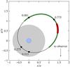 |
Fig. 1 Orbital geometry of LS I +61 303 looking down on the orbital plane showing the orbit of the compact object around the Be star in units of the orbital semi-major axis. The positions labeled with the orbital phase correspond to periastron, apastron, and inferior and superior conjunctions. The X-ray/VHE multiwavelength campaign covered the phase range shown in green (0.43 < φ < 1.13), while the phase range of the VHE emission outburst is shown in red (0.6 < φ < 0.7). The Be star (blue circle) and the equatorial wind (grey circle) are shown assuming an equatorial disk radius of rd = 7 R ⋆ . |
Because of the many factors involved, simultaneous X-ray/VHE observations are a useful mean to start to disentangle the physics of the high-energy emission in gamma-ray binaries. However, the combined effect of short-term variability in the X-ray domain and night-to-night variability in the VHE domain has precluded a clear detection of X-ray/VHE emission correlation from archival observations. In 2007, a campaign of simultaneous observations with the MAGIC Cherenkov telescope and the XMM-Newton and Swift X-ray satellites revealed a correlation between the X-ray and VHE bands (Anderhub et al. 2009). The suggestion that the emission in both energy bands comes from the same population of accelerated particles (Anderhub et al. 2009, see discussion) makes these observations an ideal data set to test the properties of the X-ray/VHE emitter in LS I +61 303. It is worth noting that the need of only one leptonic population to explain the X-ray and the VHE emission would be against lepto-hadronic models (e.g. Chernyakova et al. 2006).
In this work, we present the results of the application of a leptonic one zone model to explain the measured light curves and spectra from these observations. Our goal is to obtain the physical parameters of the emitter robustly by making as few assumptions as possible.
2. Simultaneous X-ray/VHE observations
LS I +61 303 was observed during ~60% of an orbital period simultaneously in the VHE and X-ray bands in September 2007 (Anderhub et al. 2009). During a first part of the campaign (0.43 < φ < 0.7), the MAGIC Cherenkov telescope observed the source for three hours every night and simultaneous XMM-Newton observations were performed. During a second part (0.71 < φ < 1.13) the X-ray observations were performed with Swift/XRT. The observation times were of about 15 ks for the XMM-Newton observations and of about 3 ks for the Swift/XRT observations. The longer observations and higher effective area of XMM-Newton resulted in much higher statistics than the measurements from Swift/XRT. To take into account the variability that the source shows on short time scales in the X-ray band when comparing these fluxes to the VHE measurements, the rms count rate variability of the X-ray light curve was considered in addition to the statistical uncertainty in the flux measurement to obtain realistic flux uncertainties (see Anderhub et al. 2009, for details). Using this method, the X-ray flux uncertainties take values between 6% and 25% of the flux. The simultaneous campaign revealed very similar light curves in the X-ray and VHE bands: a first outburst at φ = 0.62 with a rise time below 20 h and a decay of about two days; and a second broader outburst spanning a few days between phases 0.8 and 1.1 with lower peak flux than the first. The correlation coefficient between the two bands for the first outburst was found to be r = 0.97, whereas taking all simultaneous observations lowered the value to r = 0.81.
Although all X-ray observations resulted in a clear detection, some of the VHE flux measurements have a significance below 2σ. For these cases we will consider the 95% CL (confidence level) upper limits calculated by Jogler (2009). The detailed fluxes and uncertainties of the X-ray and VHE light curves may be found in Tables 1 and 2 of Anderhub et al. (2009) and the VHE upper limits in Table A.1 of Jogler (2009).
The sensitivity of VHE observations precludes obtaining nightly spectra, and only a spectrum combining the observations with phases between 0.6 and 0.7 was published by Anderhub et al. (2009). In order to obtain a simultaneous SED, we extracted an XMM–Newton spectrum of the source for the three X-ray observations that correspond to the MAGIC spectrum. We filtered the data using SAS v10.0 and extracted three individual spectra from the pn instrument. We used the SAS tool efluxer to convert the spectra from counts vs. channel into physical units (flux density vs. energy), averaged the three unbinned spectra and then grouped the bins to a signal-to-noise ratio of 20. In order to compare the measured spectrum to the computed intrinsic spectrum, we deabsorbed the former using the wabs FORTRAN subroutine provided with Xspec v12.0 (Arnaud 1996). We used a column density of NH = 5 × 1021 cm-2 obtained from the average of the individual fits of an absorbed power law to the three observations. This column density is consistent with that of the ISM alone (Paredes et al. 2007).
3. Model description
The discovery of a correlation between the X-ray and VHE bands points towards a common mechanism of emission modulation at both bands. In a leptonic scenario, the fast and simultaneous changes in flux in both bands indicate that the modulation mechanism has to directly affect the emission level of the Inverse Compton (IC) and synchrotron processes. Assuming constant injection, a way to obtain correlated X-ray and VHE emission is through a modulation of the number of emitting particles by dominant adiabatic losses, which would be ultimately related to the (magneto)hydrodynamical processes in the accelerator and emitter regions. These processes may be related, for instance, to the interaction of the pulsar wind or the black hole jet with the stellar wind of the massive companion. The hard X-ray spectrum with photon index Γ ≈ 1.5 also points towards dominant adiabatic losses, which imply an injection electron index of αe ≈ 2. In the regime of dominant adiabatic losses the emitted X-ray flux is proportional to the number of emitting particles, so the orbital dependency of adiabatic losses can be inferred from the X-ray light curve. Dominant adiabatic losses are not uncommon when modelling gamma-ray binaries. They have also been invoked to explain the variations of the X-ray and VHE fluxes in the gamma-ray binaries PSR B1259-63 and LS 5039 by Khangulyan et al. (2007) (see also Kerschhaggl 2011) and Takahashi et al. (2009), respectively. We note that, as explained in Sect. 3.4, the IC emission will be additionally modulated by the changes in seed photon density along the orbit as well as the geometrical effects of the location of the emitter along the orbit.
For the sake of simplicity, and given how little we know about the exact properties of the particle accelerator and the non-thermal emitter in LS I +61 303, we will here assume a constant particle injection spectrum and emitter magnetic field along the orbit. We will also adopt one leptonic population cooling down under variable adiabatic losses at the location of the emitter, which will be approximated as homogeneous and point-like.
The orbital parameters were adopted from Aragona et al. (2009) with an inclination angle of i = 45°. We will also discuss other possibilities regarding the inclination angle, in particular the extremes of the allowed range 15° ≲ i ≲ 60° considered by Casares et al. (2005). A sketch of the orbital configuration of LS I +61 303 can be seen in Fig. 1 with the phase ranges of the simultaneous X-ray/VHE campaign indicated. The equatorial wind disk in binaries of the characteristics of LS I +61 303 is expected to be truncated at a radius of rd = 5 R ⋆ (Grundstrom et al. 2007). However, the variability in the equivalent width of the Hα line indicates that its radius can vary between 4.5 R ⋆ and 7 R ⋆ (Zdziarski et al. 2010; Sierpowska-Bartosik & Torres 2009). A variable red shoulder in the Hα line (McSwain et al. 2010) could point towards the creation of a tidal stream in the equatorial disk because of the proximity of the compact at periastron that eventually falls back onto the disk at later phases. Even at its largest possible radius of 7 R ⋆ , as assumed in Fig. 1, the equatorial disk does not affect the phase ranges of the observations we are considering, and thus we will not include it in our model.
3.1. Adiabatic cooling
One of the remarkable features of the VHE light curve of LS I +61 303 is the lack of
detectable emission during periastron (Albert et al.
2009). IC emission is very effective at this phase owing to the high stellar
photon density, so the lack of emission means that either it is strongly absorbed or that
the number of accelerated electrons falls drastically. However, the angular dependency of
the pair production process, ∝ (1 − cosψ) for the interaction rate and
∝ (1 − cosψ)-1 for the gamma-ray energy threshold
(where ψ is the interaction angle of the incoming photons), implies
that absorption is very low for phases immediately after periastron even under the dense
seed photon field of the star (see Sect. 3.5 for
details on the calculation of pair production absorption). Inverse Compton emission also
has a dependency on the angle between the seed photon and the accelerated electron and
would be lower during these phases, but this effect is diminished at higher energies when
scattering takes place in the deep Klein-Nishina regime (see Fig. 5 in Khangulyan et al. 2008b). A reduction in the number of
accelerated particles is required to explain the lack of VHE emission around periastron.
Although the X-ray flux during periastron is around half of the peak flux during the
periodic outbursts, the non-detection of VHE emission during periastron places an upper
limit at only a 10% of the outburst peak VHE flux. Taking all this into account, we will
assume that in the context of one electron population the X-ray/VHE correlation is only
valid for the X-ray excess flux above a certain quiescent or pedestal emission. Therefore,
the number of emitting particles responsible for this excess X-ray flux is lower and their
VHE emission remains at non-detectable levels around periastron. This reasoning is
supported by the X-ray/VHE correlation found by Anderhub
et al. (2009), in which the constant term of the linear correlation is
 .
Considering that some of the X-ray observations are below this constant term, we took the
pedestal flux value to be
Fped = 11.5 × 10⁻¹²ergcm-2s-1.
.
Considering that some of the X-ray observations are below this constant term, we took the
pedestal flux value to be
Fped = 11.5 × 10⁻¹²ergcm-2s-1.
As mentioned above, a scenario with dominant adiabatic losses is a very good candidate mechanism to explain the correlation characteristics of the source. When considering a system with constant magnetic field and constant injected electron spectrum, the only modulation in synchrotron radiation is due to the modulation of the dominant cooling process that results in a modulation of the (evolved) stationary electron distribution. For dominant adiabatic losses and a constant injection rate, the X-ray flux will be proportional to the adiabatic cooling time tad. A consistent calculation of tad would require knowledge of the exact nature of the source and the (magneto)hydrodynamical processes that take place there. One can however infer tad along the orbit by taking it proportional to the excess flux above the pedestal FX − Fped, which is independent of the electron energy. For the phases covered by the X-ray observations we derived a smooth curve following the behaviour of the X-ray fluxes. For the phases outside the campaign coverage we assumed a flat light curve consistent with the first four observations at phases 0.43 to 0.59 and the last observation at phase 0.13. Choosing the ratio tad/(FX − Fped) as small as possible while keeping the adiabatic losses dominant allows us to put a lower limit on the injected luminosity budget. This choice of the ratio tad/(FX − Fped) yields adiabatic loss time scales of between 35 and 500 s. Figure 2 shows the orbital evolution of the cooling time scales inferred for adiabatic and calculated for IC and synchrotron losses. The adiabatic cooling time is independent of the electron energy, but for synchrotron and IC the cooling time scales are given at Ee = 1012 eV. This energy corresponds to electrons that emit in the X-ray band through synchrotron and in the VHE band through IC.
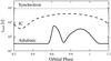 |
Fig. 2 Cooling times along the orbit for adiabatic (solid), synchrotron (dotted) and IC (dashed). The synchrotron and IC cooling times are shown at Ee = 1012 eV. This energy corresponds to electrons that emit in the X-ray band through synchrotron and in the VHE band through IC. |
3.2. Particle energy distribution
The radiation emitted by a population of non-thermal particles arises from the
contribution of electrons of different ages. As electrons loose energy through radiative
or adiabatic cooling processes, an evolved particle energy distribution, different from
the injected particle spectrum (Q(γ), taken here
constant in time), arises. The evolved particle spectrum
n(γe,t) can be obtained
from Q(γ) through the following equation (Ginzburg & Syrovatskii 1964):  (1)where
 is the sum of the energy loss rates for IC, synchrotron and adiabatic processes and
Q(γe) is the acceleration rate. Since
little is known about the acceleration process responsible for particle acceleration in
LS I +61 303, we assume a constant particle injection spectrum along the orbit. We adopt a
phenomenological electron injection spectrum
Q(γe) consisting of a power law function
with an exponential high energy cutoff:
is the sum of the energy loss rates for IC, synchrotron and adiabatic processes and
Q(γe) is the acceleration rate. Since
little is known about the acceleration process responsible for particle acceleration in
LS I +61 303, we assume a constant particle injection spectrum along the orbit. We adopt a
phenomenological electron injection spectrum
Q(γe) consisting of a power law function
with an exponential high energy cutoff:  . The
maximum electron energy Ee,max is obtained from the balance of
acceleration and energy loss rates, thus establishing a cutoff in the accelerated particle
energy spectrum (see Sect. 3.3);
αe is typically ~2 in the context of
non-relativistic first order Fermi acceleration (see, e.g., Drury 1983); and Q0 is the normalization of
the function, which we keep constant along the orbit.
. The
maximum electron energy Ee,max is obtained from the balance of
acceleration and energy loss rates, thus establishing a cutoff in the accelerated particle
energy spectrum (see Sect. 3.3);
αe is typically ~2 in the context of
non-relativistic first order Fermi acceleration (see, e.g., Drury 1983); and Q0 is the normalization of
the function, which we keep constant along the orbit.
For LS I +61 303 the adiabatic and radiative cooling time scales of high-energy electrons
are much shorter than the orbital period, and thus we can calculate the steady-state
electron energy distribution along the orbit omitting the first term in Eq. (1) and solving for
n(γe): 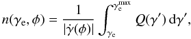 (2)The resulting
n(γe,φ) is the evolved
particle spectrum for which the emitted radiation properties are calculated along the
orbit.
(2)The resulting
n(γe,φ) is the evolved
particle spectrum for which the emitted radiation properties are calculated along the
orbit.
3.3. Maximum electron energy
The VHE gamma-ray energy spectrum of LS I +61 303 extends up to
Eγ ~ 10 TeV (see Acciari et al. 2009) without a break in the spectrum,
indicating that electrons must be accelerated up to energies beyond 10 TeV. The
acceleration of electrons has to be faster than the cooling times of the different cooling
mechanisms so that the electrons can reach these very high energies. The maximum electron
energy will be that for which
tacc = tcool. The acceleration
time of electrons can be characterized as
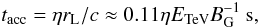 (3)where
rL = E/eB is the Larmor
radius, BG is the magnetic field in Gauss and
ETeV is the electron energy in TeV. The dimensionless
constant η ≥ 1 indicates the efficiency of the acceleration process,
where η → 1 corresponds to the maximum possible acceleration rate allowed
by classical electrodynamics and
η = 2π(vs/c)-2
for parallel non-relativistic diffusive shocks in the Bohm regime (Drury 1983).
(3)where
rL = E/eB is the Larmor
radius, BG is the magnetic field in Gauss and
ETeV is the electron energy in TeV. The dimensionless
constant η ≥ 1 indicates the efficiency of the acceleration process,
where η → 1 corresponds to the maximum possible acceleration rate allowed
by classical electrodynamics and
η = 2π(vs/c)-2
for parallel non-relativistic diffusive shocks in the Bohm regime (Drury 1983).
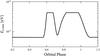 |
Fig. 3 Maximum electron energy Ee,max along the orbit taking η = 10 (see text for details). |
 (4)However, at some
points along the orbit in which adiabatic losses are smaller, synchrotron losses may
dominate at high energies, since
(4)However, at some
points along the orbit in which adiabatic losses are smaller, synchrotron losses may
dominate at high energies, since  whereas the adiabatic cooling time is constant with electron energy. In these cases, with
a synchrotron cooling time described by
whereas the adiabatic cooling time is constant with electron energy. In these cases, with
a synchrotron cooling time described by
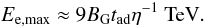
 (5)the balance
tacc = tsyn results in a maximum
energy of
(5)the balance
tacc = tsyn results in a maximum
energy of  (6)Inverse Compton energy
losses at the relevant energies are smaller than to the synchrotron and adiabatic losses.
At each point along the orbit, all relevant time scales are evaluated and the
corresponding Ee,max is obtained, which in this work
characterizes the position of the cutoff in the injected particle spectrum through an
exponential cutoff. The adiabatic cooling times inferred from the X-ray light curve range
from a few tens to a few hundred seconds. When considering the requirement that
acceleration takes place up to electron energies of 10 TeV, we can see that the
accelerator required must be quite efficient with η ≈ 7–130 depending on
the orbital phase. Since we are assuming that the injection is constant, we also expect
the acceleration rate to be constant and have chosen a value of η = 10 to
perform the energy cutoff calculations along the orbit, which would correspond to
acceleration in a parallel diffusive shock with velocity of
~0.8c (therefore favoring a mildly relativistic shock). The
orbital dependency of the maximum electron energy for η = 10 is shown in
Fig. 3. During periods of low X-ray flux
Ee,max has a behaviour proportional to
tad (see Fig. 2).
During the outburst peaks, on the other hand, high energy losses are dominated by
synchrotron and the cutoff is constant (following Eq. (6) for constant magnetic field).
(6)Inverse Compton energy
losses at the relevant energies are smaller than to the synchrotron and adiabatic losses.
At each point along the orbit, all relevant time scales are evaluated and the
corresponding Ee,max is obtained, which in this work
characterizes the position of the cutoff in the injected particle spectrum through an
exponential cutoff. The adiabatic cooling times inferred from the X-ray light curve range
from a few tens to a few hundred seconds. When considering the requirement that
acceleration takes place up to electron energies of 10 TeV, we can see that the
accelerator required must be quite efficient with η ≈ 7–130 depending on
the orbital phase. Since we are assuming that the injection is constant, we also expect
the acceleration rate to be constant and have chosen a value of η = 10 to
perform the energy cutoff calculations along the orbit, which would correspond to
acceleration in a parallel diffusive shock with velocity of
~0.8c (therefore favoring a mildly relativistic shock). The
orbital dependency of the maximum electron energy for η = 10 is shown in
Fig. 3. During periods of low X-ray flux
Ee,max has a behaviour proportional to
tad (see Fig. 2).
During the outburst peaks, on the other hand, high energy losses are dominated by
synchrotron and the cutoff is constant (following Eq. (6) for constant magnetic field).
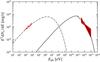 |
Fig. 4 Computed SED averaged over the three observation periods during the first outburst (phases 0.62, 0.66 and 0.70), with synchrotron (dot-dashed), IC (solid) and non-absorbed IC (dashed) components. The calculations were performed with i = 45° and B = 0.22 G. The crosses show the XMM–Newton EPIC-pn spectrum averaged over three observations and deabsorbed taking NH = 5 × 1021 cm-2. To compare the measured flux to the excess computed X-ray flux, we subtracted a pedestal power law spectrum corresponding to a 0.3 − 10 keV flux of 11.5 × 10⁻¹²ergcm-2s-1. The MAGIC simultaneous spectrum is shown as a red bow-tie. |
3.4. Synchrotron and IC emission
For each position along the orbit, we calculate the emitted synchrotron spectrum from the evolved particle distribution and the magnetic field. Synchrotron emission in the X-ray range will be generally characterized by a photon index of ΓX = (αe + 1)/2 ≈ 1.5. The orbital dependence of the electron maximum energy will affect the shape of the spectrum, typically hardening (softening) it for high (low) fluxes, which correspond to lower (higher) adiabatic losses and therefore a higher (lower) maximum electron energy. However, since the cutoff in the particle distribution is located at energies significantly higher than those responsible for X-ray emission, this effect is small in the X-ray energy band (ΔΓX ~ 0.2).
We calculate the IC component of the spectrum using the anisotropic cross section and the
stellar radiation field (blackbody radiation at kT = 2 eV and
L ⋆ = 1038 erg s-1)
as the source of seed photons for the interaction. Following Eqs. (20) and (21) of Aharonian & Atoyan (1981), the photon spectrum
emitted by a population of isotropically distributed electrons can be described with a
precision better than 3% (for ϵ ≫ ϵ0 and
γ ≫ 1) by 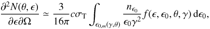 (7)where ϵ
and ϵ0 are the energies of the scattered and incident photons,
respectively, in units of
mec2,
θ is the scattering angle, σT is the
Thomson cross section, nϵ0 is the
number density of the stellar photon field,
(7)where ϵ
and ϵ0 are the energies of the scattered and incident photons,
respectively, in units of
mec2,
θ is the scattering angle, σT is the
Thomson cross section, nϵ0 is the
number density of the stellar photon field,
![Mathematical equation: \begin{equation} \epsilon_{0,m}(\gamma,\theta)=\frac{\epsilon}{2(1-\cos\theta)\gamma^2[1-\epsilon/\gamma]}, \end{equation}](/articles/aa/full_html/2011/03/aa15373-10/aa15373-10-eq90.png) (8)and
(8)and
 (9)where
bθ = 2(1 − cosθ)ϵ0γ
and z = ϵ/γ. For a blackbody seed
photon distribution, the shape of the resulting emitted spectrum only depends on the
parameter bθ and the relativistic electron
energy distribution.
(9)where
bθ = 2(1 − cosθ)ϵ0γ
and z = ϵ/γ. For a blackbody seed
photon distribution, the shape of the resulting emitted spectrum only depends on the
parameter bθ and the relativistic electron
energy distribution.
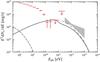 |
Fig. 5 Computed SED averaged over the whole orbit with synchrotron (dot-dashed), IC (solid) and non-absorbed IC (dashed) components, calculated with the same parameters as in Fig. 4. The crosses and upper limits indicate the phase-averaged Fermi/LAT spectrum. The MAGIC VHE spectrum during the outburst is shown as a bow-tie. It must be noted that the MAGIC spectrum corresponds to different phases than the computed SED and is shown as a reference to Fig. 4. |
3.5. Pair production absorption
The intense radiation field can also absorb very high energy γ-ray
emission through pair production γγ → e + e −
(Gould & Schréder 1967). An exploration
of the effects that this absorption can have on the observed spectrum of gamma-ray
binaries can be found in Bosch-Ramon & Khangulyan
(2009) and references therein. The differential opacity for an emitted
γ-ray of energy ϵ is given by  (10)where
l is the distance along the line of sight,
ϵ0 is the energy of the stellar photon, ψ
is the interaction angle and the absorption cross section can be represented in the form:
(10)where
l is the distance along the line of sight,
ϵ0 is the energy of the stellar photon, ψ
is the interaction angle and the absorption cross section can be represented in the form:
![Mathematical equation: \begin{equation} \sigma_{\gamma\gamma}=\frac{\pi r^2_{\rm e}}{2}\left(1-\beta^2\right) \left[2\beta\left(\beta^2-2\right)+\left(3-\beta^4\right) \ln\left(\frac{1+\beta}{1-\beta}\right)\right], \label{eq:ggsig} \end{equation}](/articles/aa/full_html/2011/03/aa15373-10/aa15373-10-eq99.png) (11)where
β = (1 − 1/s)1/2, and
s = ϵϵ0(1 − cosψ)/2.
Pair production can only occur for s > 1, when the centre of mass
energy of the incoming photons is sufficiently high to create an electron positron pair.
The cross section maximum takes place for s ≃ 3.5, with a value of
σγγ ≃ 0.2σT,
and then decreases for s ≫ 1.
(11)where
β = (1 − 1/s)1/2, and
s = ϵϵ0(1 − cosψ)/2.
Pair production can only occur for s > 1, when the centre of mass
energy of the incoming photons is sufficiently high to create an electron positron pair.
The cross section maximum takes place for s ≃ 3.5, with a value of
σγγ ≃ 0.2σT,
and then decreases for s ≫ 1.
The optical depth owing to pair production τγγ is calculated at each point along the orbit by integrating the differential opacity (Eq. (10)) along the line of sight and over the blackbody seed photon distribution. The attenuation factor κ = exp( − τγγ) is applied to the intrinsic IC spectrum (dashed line in Fig. 4) to obtain the spectrum emitted out of the binary system (solid line in Fig. 4).
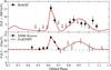 |
Fig. 6 Top: computed VHE light curve (red line) and observed VHE light curve by MAGIC in units of 10-12ph/cm2/s. Observations with a significance above 2σ are shown in filled squares, while 95% CL upper limits are shown otherwise. Bottom: computed X-ray light curve (red line) and X-ray light curve observed during the multiwavelength campaign with XMM–Newton (filled circles) and Swift/XRT (open circles) in units of 10-12erg/cm2/s. The pedestal flux is indicated by a horizontal dashed line. All error bars correspond to 1σ uncertainties. The same parameters as in Fig. 4 are used for both panels. |
4. Results
As seen in Fig. 6, we were able to reproduce the X-ray and VHE light curves obtained during the 2007 multiwavelength campaign. Although the good agreement with the X-ray light curve is expected because we derived the dominant adiabatic losses from the observed X-ray fluxes, the VHE light curve is a prediction of the model taking into account the binary geometry, the stellar photon field, and the non-thermal particle distribution. Furthermore, the spectral indices in the X-ray and VHE energy bands for the outburst at phases 0.6 < φ < 0.7 are well reproduced, as can be seen in Fig. 4.
4.1. Electron population
We found that the best fit to the X-ray and VHE photon indices can be obtained by taking a particle energy distribution with slope αe = 2.1. As mentioned above, the photon index in the X-ray band directly depends on the particle index of the parent electron population. In the X-ray band, the observations show a photon index between 1.58 ± 0.02 and 1.66 ± 0.02 (plus a 1.85 ± 0.02 outlier) for the XMM-Newton observations, which is anti-correlated with the X-ray flux. The time-dependent energy cutoff given by the variability of cooling time scales provides a small time dependent variation of the photon index through a modification of the shape of the spectrum. Regarding the VHE observations, the measured photon index is 2.7 ± 0.3stat ± 0.2sys for the three observations during the first outburst. Because absorption is low at the orbital phases of the maximum, the photon index is determined by αe and the IC interaction angle. The parent particle population with αe = 2.1 results in computed X-ray photon indices in the range 1.55–1.67 and reproduces the observed anti-correlation between ΓX and FX. In the VHE band the adopted αe results in photon indices in the range 2.6–2.8 for high-flux phases, whereas the spectrum is much softer for low flux phases because of the lower energy cutoff. Figure 4 presents the SED averaged over the phase ranges of the three simultaneous observations during the first outburst (phases 0.62, 0.66 and 0.70), and shows that both the flux levels and the photon indices at X-ray and VHE are well reproduced.
We found that the phase-averaged SED calculated using a power law with αe = 2.1 and a high-energy cutoff produces a flux too high in energies between 10 and 100 GeV when compared to the phase-averaged spectrum measured by Fermi/LAT (Abdo et al. 2009). The GeV spectrum and fluxes along the orbit appear incompatible with one leptonic population. A way to avoid this excess flux is to consider the electron injection spectrum described by a broken power law with a harder particle index below Ee = 4 × 10¹¹ eV. We found that the softest particle index for which the computed GeV spectrum is compatible with the Fermi/LAT measurement is αe ≲ 1.8. It must be noted that this change in the particle index at low energies does not affect the spectrum of particles that emit in the X-ray and VHE bands through synchrotron and IC, respectively. The Fermi/LAT spectrum along with the computed phase averaged SED is shown in Fig. 5. The phase-averaged Fermi/LAT cannot be easily compared with the peak spectrum shown in Fig. 4 because the X-ray/VHE and GeV measurements are not simultaneous. Furthermore, the orbital variability of the GeV spectrum at higher energies (i.e., the shape of the cutoff) has not been clearly established by Abdo et al. (2009), and a phase-resolved spectrum cannot be derived from a phase averaged-spectrum.
4.2. Magnetic field
The X-ray/VHE flux ratio is a very sensitive indicator of the magnetic field in the emitter. We found the magnetic field that best describes the observed light curves by performing a exploration of the parameter space of B and the normalization of the injected particle spectrum Q0. For each (B,Q0) pair we calculated the X-ray and VHE light curves and estimated the goodness-of-fit to the observed flux points using a χ2 test. The observed light curves are best described using an ambient magnetic field of B = 0.22 G. It is not trivial to set a formal uncertainty range on this value because of the unknown number of constraints that should be considered (e.g., the shape used for the adiabatic cooling curve). However, we see that for variations of the order of 0.05 G around the best-fit value of B = 0.22 G the observed X-ray and VHE light curves are no longer well described by the computed ones.
4.3. Injection energy budget
The adopted luminosity in injected accelerated particles is around 2 × 1035 erg s-1 along the whole orbit. The computed emission bolometric luminosity, on the other hand, varies between ~1034 and ~1.5 × 1035 erg s-1. Note that the adopted injected luminosity is only a lower limit because we arbitrarily chose the lowest ratio between the X-ray flux and the adiabatic cooling time scale. For higher adiabatic losses (while still proportional to X-ray emission), the emitted spectrum would be equivalent but the required injected luminosity would be higher.
The dominant energy band in the broad-band SED of LS I +61 303 is the MeV-GeV region. Using the gamma-ray spectrum measured by Fermi/LAT (Abdo et al. 2009) we can obtain a lower limit on the power available for particle acceleration. The observed energy flux above 100 MeV is G100 ≃ 4.1 × 10⁻¹⁰ erg cm-2 s-1, resulting in an observed luminosity of 2 × 1035 erg s-1. Given this high luminosity, it is natural to think than the acceleration mechanism at play is able to provide a similar power to the X-ray and VHE emitting electrons.
5. Discussion
5.1. Adiabatic time scales
The orbital variability and range of adiabatic losses may be used to pose constraints on the hydrodynamical properties of the various scenarios proposed for LS I +61 303. Hydrodynamical calculations have been performed in the binary pulsar scenario (Bogovalov et al. 2008; Khangulyan et al. 2008a) and for the interaction of a microquasar jet with the wind of a young star (Perucho & Bosch-Ramon 2008; Perucho et al. 2010). However, for LS I +61 303 it is difficult to calculate the adiabatic losses in each of the mentioned scenarios because of the uncertainties in the properties of the Be stellar wind and the relativistic outflows.
In our phenomenological framework, we find that adiabatic loss time scales range
between 35 and 500 s, as seen in Fig. 2. Whereas it
is difficult to relate these time scales to those arising from complex geometries
(e.g. shocked pulsar wind or a microquasar jet), we can use the simple model of an
expanding sphere to obtain insight on relevant emitter properties. The adiabatic loss time
scale tad is related to the typical scale of the emitter
Rem and its expansion velocity
vexp through
tad = Rem/vexp.
While the size of the emitting region is unknown, the fact that a one-zone emitter located
at the compact object position can successfully explain the X-ray/VHE emission indicates
that the region must be small compared with the orbital separation. Considering an
emitting region with a radius 10% of the orbital separation we obtain a range of radii
between ~3 × 1011 cm (at periastron) and
~9 × 1011 cm (at apastron). For these sizes, the maximum expansion
velocities would be required for the shortest adiabatic cooling time scale, i.e. 35 s. At
apastron the expansion would need to be highly relativistic, with a velocity of
0.85c (similar to the relativistic sound speed
 ),
corresponding to a Lorentz factor of Γ = 1.89, whereas for periastron it would be mildly
relativistic at 0.29c. For the longer adiabatic loss time scales of
hundreds of seconds, the required expansion velocities would be much lower, of the order
of 0.01c–0.06c. A change in the size of the emitter
could be caused by the change in external pressure from the stellar wind, resulting in a
larger emitter at apastron (Takahashi et al. 2009).
This would explain the location of the X-ray/VHE outbursts around apastron, but it is not
clear which magnetohydrodynamical process is responsible for the variation of the
adiabatic loss time scale of more than an order of magnitude in 20 h. Wind clumping can be
considered as a source of pressure variability, as suggested by Zdziarski et al. (2010), but it would not explain the constant location
of the X-ray/VHE outburst (0.6 < φ < 0.7) orbit after
orbit. On the other hand, a transition of the emitter from a region dominated by polar
wind to a region dominated by equatorial wind, or vice versa, could give rise to such a
fast change in wind pressure. In addition, there could be other yet unknown properties of
the stellar wind, as shown by the recent detection of a variable red shoulder in the
Hα line by McSwain et al.
(2010), which could be related to a tidal stream in the equatorial wind falling
back onto the disk.
),
corresponding to a Lorentz factor of Γ = 1.89, whereas for periastron it would be mildly
relativistic at 0.29c. For the longer adiabatic loss time scales of
hundreds of seconds, the required expansion velocities would be much lower, of the order
of 0.01c–0.06c. A change in the size of the emitter
could be caused by the change in external pressure from the stellar wind, resulting in a
larger emitter at apastron (Takahashi et al. 2009).
This would explain the location of the X-ray/VHE outbursts around apastron, but it is not
clear which magnetohydrodynamical process is responsible for the variation of the
adiabatic loss time scale of more than an order of magnitude in 20 h. Wind clumping can be
considered as a source of pressure variability, as suggested by Zdziarski et al. (2010), but it would not explain the constant location
of the X-ray/VHE outburst (0.6 < φ < 0.7) orbit after
orbit. On the other hand, a transition of the emitter from a region dominated by polar
wind to a region dominated by equatorial wind, or vice versa, could give rise to such a
fast change in wind pressure. In addition, there could be other yet unknown properties of
the stellar wind, as shown by the recent detection of a variable red shoulder in the
Hα line by McSwain et al.
(2010), which could be related to a tidal stream in the equatorial wind falling
back onto the disk.
5.2. Energetics
The energetics of the system, regardless of the acceleration mechanism, are able to provide the required injected power used in our model given the high flux in the MeV-GeV band (see Sect. 4.3).
The pulsar-like spectrum of LS I +61 303 in the GeV band (power law with exponential
cutoff at a few GeV) prompted Abdo et al. (2009) to
consider a magnetospheric origin for the HE gamma-ray emission. In this scenario we can
gain some insight on the spin-down luminosity of the putative pulsar from the HE gamma-ray
luminosity. The observed energy flux G100 from magnetospheric
emission can be related to the emitted gamma-ray
luminosity Lγ as  (12)where
fΩ is a beaming correction factor that depends on the
geometry of the emitter, the magnetic angle α and the Earth viewing angle
ζE. The emitted gamma-ray luminosity is related to the
pulsar spin-down luminosity through the gamma-ray efficiency
ηγ = Lγ/Ė.
A trend was found from EGRET observations that the efficiency scaled as
Ė −1/2 (Thompson et al.
1999), and this was later confirmed (at least for
Ė > 1034 erg s-1) by
Fermi/LAT arriving to
ηγ ≃ 0.034(Ė/1036 ergs-1) − 1/2
(Abdo et al. 2010). Using this relation,
Ė can be inferred from Lγ
as
(12)where
fΩ is a beaming correction factor that depends on the
geometry of the emitter, the magnetic angle α and the Earth viewing angle
ζE. The emitted gamma-ray luminosity is related to the
pulsar spin-down luminosity through the gamma-ray efficiency
ηγ = Lγ/Ė.
A trend was found from EGRET observations that the efficiency scaled as
Ė −1/2 (Thompson et al.
1999), and this was later confirmed (at least for
Ė > 1034 erg s-1) by
Fermi/LAT arriving to
ηγ ≃ 0.034(Ė/1036 ergs-1) − 1/2
(Abdo et al. 2010). Using this relation,
Ė can be inferred from Lγ
as  . From
the LS I +61 303 phase-averaged gamma-ray spectrum measured by Abdo et al. (2009) we obtain
G100 ≃ 4.1 × 10⁻¹⁰ erg cm-2 s-1,
from which
Lγ ≃ 2 × 1035fΩ erg s-1.
Following these considerations, the spin-down luminosity inferred from the
Fermi/LAT observations is of
. From
the LS I +61 303 phase-averaged gamma-ray spectrum measured by Abdo et al. (2009) we obtain
G100 ≃ 4.1 × 10⁻¹⁰ erg cm-2 s-1,
from which
Lγ ≃ 2 × 1035fΩ erg s-1.
Following these considerations, the spin-down luminosity inferred from the
Fermi/LAT observations is of  erg s-1.
Traditionally (e.g. polar cap models) it was assumed that the gamma-ray beam covers a
solid angle of 1 sr uniformly, so
fΩ = 1/(4π) ≃ 0.08, which would result in
a spin-down luminosity of Ė ≃ 2 × 1035 erg s-1.
However, more modern pulsar beaming models (e.g. slot gap and outer gap models) have
fΩ ~ 1 for many viewing angles (Watters et al. 2009), which would result in a more
energetic pulsar with Ė ≃ 3 × 1037 erg s-1. The
fact that the cutoff of the spectrum is located at high energies
(Ecutoff = 6.3 ± 1.1 GeV) points to a high-altitude location
for gamma-ray emission, since emission beyond a few GeV is very difficult close to the
neutron star because of strong attenuation from
γ − B → e + e − absorption
(Baring 2004). The general trend in the
Fermi/LAT pulsar sample (Abdo et al.
2010) also points towards a high-altitude location, so we favour slot gap or
outer gap models for which the spin-down luminosity of the putative pulsar in LS I +61 303
would be of Ė ≃ 3 × 1037 erg s-1. Even though the
Fermi/LAT observations do not completely constrain the spin-down
luminosity of the putative pulsar, the power available for particle acceleration is high.
In the favoured scenario of Ė ≃ 3 × 1037 erg s-1,
assuming that the power in injected electrons constitutes only a fraction 10-2
of the spin-down luminosity (e.g. Sierpowska-Bartosik
& Torres 2008), the power in relativistic electron would be larger than
our requirement of
Linj = 2 × 1035 erg s-1.
erg s-1.
Traditionally (e.g. polar cap models) it was assumed that the gamma-ray beam covers a
solid angle of 1 sr uniformly, so
fΩ = 1/(4π) ≃ 0.08, which would result in
a spin-down luminosity of Ė ≃ 2 × 1035 erg s-1.
However, more modern pulsar beaming models (e.g. slot gap and outer gap models) have
fΩ ~ 1 for many viewing angles (Watters et al. 2009), which would result in a more
energetic pulsar with Ė ≃ 3 × 1037 erg s-1. The
fact that the cutoff of the spectrum is located at high energies
(Ecutoff = 6.3 ± 1.1 GeV) points to a high-altitude location
for gamma-ray emission, since emission beyond a few GeV is very difficult close to the
neutron star because of strong attenuation from
γ − B → e + e − absorption
(Baring 2004). The general trend in the
Fermi/LAT pulsar sample (Abdo et al.
2010) also points towards a high-altitude location, so we favour slot gap or
outer gap models for which the spin-down luminosity of the putative pulsar in LS I +61 303
would be of Ė ≃ 3 × 1037 erg s-1. Even though the
Fermi/LAT observations do not completely constrain the spin-down
luminosity of the putative pulsar, the power available for particle acceleration is high.
In the favoured scenario of Ė ≃ 3 × 1037 erg s-1,
assuming that the power in injected electrons constitutes only a fraction 10-2
of the spin-down luminosity (e.g. Sierpowska-Bartosik
& Torres 2008), the power in relativistic electron would be larger than
our requirement of
Linj = 2 × 1035 erg s-1.
Another possibility is that instead of a magnetospheric origin, the emission detected by Fermi/LAT has an Inverse Compton origin. In this case the efficiency between the spin-down luminosity of the putative pulsar and the observed IC luminosity is expected to be of 1–10%. Considering the observed luminosity of a few times 1035 erg s-1, the pulsar would need to have a spin-down luminosity of the order of 1037 erg s-1.
The higher values of spin-down luminosities pose a problem for the binary pulsar scenario
regarding the shape of the detected radio emission. Dhawan
et al. (2006) strongly argued that the rotating cometary-like tail they detected
in VLBA observations was related to the shocked pulsar wind contained by the stellar wind.
Romero et al. (2007) already questioned the
ability of the stellar wind to contain the pulsar wind from the results of
three-dimensional hydrodynamical simulations even when considering a significantly lower
spin-down luminosity of 1036 erg s-1. The shape of the interaction
region between the stellar and pulsar winds is determined by the ratio of wind momentum
fluxes  (13)where
Ṁ ⋆ and
vw ⋆ are the mass-loss rate and wind
velocity of the Be star and ĖPSR is the spin-down luminosity
of the pulsar. For the polar wind, we can take
Ṁ ⋆ = 10-8M⊙yr-1
and vw ⋆ = 103 km s-1,
resulting in a wind momentum flux ratio of
ηw = 0.53(ĖPSR/1036 ergs-1)
(Romero et al. 2007). Ignoring orbital motion
(which on the other hand would give rise to small deviations in the inner region of the
interaction, see Parkin & Pittard 2008),
the opening half-angle of the interaction cone would be
(13)where
Ṁ ⋆ and
vw ⋆ are the mass-loss rate and wind
velocity of the Be star and ĖPSR is the spin-down luminosity
of the pulsar. For the polar wind, we can take
Ṁ ⋆ = 10-8M⊙yr-1
and vw ⋆ = 103 km s-1,
resulting in a wind momentum flux ratio of
ηw = 0.53(ĖPSR/1036 ergs-1)
(Romero et al. 2007). Ignoring orbital motion
(which on the other hand would give rise to small deviations in the inner region of the
interaction, see Parkin & Pittard 2008),
the opening half-angle of the interaction cone would be
 (14)as seen in analytical
models of wind interaction (e.g. Antokhin et al.
2004). For a spin-down luminosity of 1036 erg s-1 the
stellar wind would barely dominate the pulsar wind (ηw = 0.53,
θ = 62°). Considering the favoured high-altitude location for gamma-ray
production (i.e., slot gap or outer gap models) or an IC origin of the gamma-ray emission,
the pulsar spin-down luminosity is of the order of
ĖPSR ~ 1037 erg s-1. Given
this luminosity, the pulsar wind would dominate the interaction and would not be contained
by the stellar wind. The ratio of wind momentum fluxes would then be of
ηw ≃ 16 and the half-opening angle would approach 180°,
posing a completely different scenario from that usually pictured by wind interaction
models (e.g. Dubus 2006; Sierpowska-Bartosik & Torres 2009; Zdziarski et al. 2010). A lower value of the beaming correction
factor fΩ in the magnetospheric scenario could mean that the
pulsar spin-down luminosity is as low as
ĖPSR ≃ 2 × 1035 erg s-1 and thus
contained by the stellar wind. However, given the high energy of the cutoff in the
Fermi/LAT spectrum of LS I +61 303 we favour a high-altitude location
for gamma-ray production, leading to the higher value of the spin-down luminosity.
(14)as seen in analytical
models of wind interaction (e.g. Antokhin et al.
2004). For a spin-down luminosity of 1036 erg s-1 the
stellar wind would barely dominate the pulsar wind (ηw = 0.53,
θ = 62°). Considering the favoured high-altitude location for gamma-ray
production (i.e., slot gap or outer gap models) or an IC origin of the gamma-ray emission,
the pulsar spin-down luminosity is of the order of
ĖPSR ~ 1037 erg s-1. Given
this luminosity, the pulsar wind would dominate the interaction and would not be contained
by the stellar wind. The ratio of wind momentum fluxes would then be of
ηw ≃ 16 and the half-opening angle would approach 180°,
posing a completely different scenario from that usually pictured by wind interaction
models (e.g. Dubus 2006; Sierpowska-Bartosik & Torres 2009; Zdziarski et al. 2010). A lower value of the beaming correction
factor fΩ in the magnetospheric scenario could mean that the
pulsar spin-down luminosity is as low as
ĖPSR ≃ 2 × 1035 erg s-1 and thus
contained by the stellar wind. However, given the high energy of the cutoff in the
Fermi/LAT spectrum of LS I +61 303 we favour a high-altitude location
for gamma-ray production, leading to the higher value of the spin-down luminosity.
5.3. Orbital inclination
Synchrotron emission will have no dependence on the orbital inclination because we are assuming isotropic particle distribution and a fully disordered magnetic field. For IC emission, on the other hand, there is a dependence with the angle θ between the line of sight and the direction of propagation of the seed photons (i.e., the connecting line between the star and the compact object). Given the orbital configuration of LS I +61 303 (see Fig. 1), θ will not vary significantly with inclination for the phases around apastron, at which the source is detected in VHE. For γγ absorption, on the other hand, the dependency is on the angle between the directions of the VHE photon and the seed photon integrating along the line of sight out of the system. This means that absorption will show weaker orbital variability for low inclinations and stronger for high inclinations. For the flux peak observed at φ = 0.62, the optical depth of γγ absorption is practically independent of inclination at τγγ ≈ 0.2 for 500 GeV photons. However, the second, wider outburst at phases 0.8–1.1, does have an absorption dependency with inclination, with τγγ ≈ 1.4 for i = 60° but τγγ ≈ 0.3 for i = 15°. The diminished absorption at low inclinations leads to a VHE flux higher than the observed values, particularly taking into account the upper limit measurement at phase 0.8. However, given the high uncertainties of the VHE nightly fluxes, the difference between the light curves computed for i = 60° and i = 15° is of less than 1σ. Even though we do not consider it significant given the present sensibilities, deeper VHE observations with firm detections at these phases could help to constrain the inclination of the orbit.
5.4. Magnetic field
The X-ray/VHE fluxes can be explained using a constant magnetic field of B = 0.22 G. A constraint on the accelerator maximum energy can be put by requiring that the Larmor radius of the accelerated electron (rL = Ee/qBc) is contained within the accelerator size. This translates to a maximum energy of Emax = 300BGR12 TeV, where BG is the magnetic field in Gauss and R12 the accelerator radius in units of 1012 cm. For the magnetic field we found and considering an accelerator size of the order of 10% of the orbital separation, the maximum energy is well above the required 10 TeV and radiative losses dominate at high energies (see Sect. 3.3). In the binary pulsar modelling approach of Dubus (2006), the magnetic flux was considered variable along the orbit as a consequence of the variation in the distance of the wind-shock region to the pulsar. In the shocked wind region, the magnetic field values obtained were as high as 10 G. Chernyakova et al. (2006) obtain a very similar magnetic field to ours, with B = 0.25 G (B = 0.35 G) for the low (high) flux state of the source. However, the model is based on an emitting particle spectrum very soft at high energies, resulting in a synchrotron component peaking in the radio band and an IC component dominating from soft X-ray to the MeV band. They require another hadronic component to explain the VHE emission. The magnetic field in this model traces the flux ratio between radio and X-ray fluxes instead of ours, which traces the flux ratio between X-ray and VHE. On the other hand, in the microquasar approach used by Bosch-Ramon et al. (2006a), the magnetic field at the base of the jet was taken as 1 G. Most of these approaches use higher magnetic fields than the one we found to best reproduce the observational features. An explanation for this is likely the need in these models to generate both the pedestal and X-ray flux that we considered independently.
6. Summary and concluding remarks
We presented a radiation model of a single leptonic population that can successfully describe the data obtained through a simultaneous X-ray/VHE campaign on LS I +61 303 performed by MAGIC in 2007. The observed X-ray/VHE correlation indicates both that the emission at these bands may come from a single particle population and that energy losses may be dominated by adiabatic losses. By assuming a constant magnetic field and injection along the orbit, we inferred the adiabatic loss rate from the X-ray light curve and the time dependent electron maximum energy as the balance between acceleration and energy loss time scales. We found that a quite efficient accelerator (η ~ 10) is required to obtain the observed VHE spectra because of the fast adiabatic cooling. The injected electron spectrum is constant along the orbit and initially taken as a power law with a high-energy cutoff, but the Fermi/LAT HE spectrum poses a constraint on the hardness of the spectrum at lower energies, which we estimate has to be harder than αe ≃ 1.8 for electron energies below 4 × 10¹¹ eV. At higher energies, on the other hand, an index of αe = 2.1 matches the observed X-ray and VHE photon indices. The observed light curves are best reproduced using a magnetic field of B = 0.22 G. The general picture shows that the observed emission in X-ray and VHE is fully compatible with originating in the same parent particle population under dominant adiabatic losses.
The required luminosity budget in injected electrons for the computed X-ray and VHE emission is 2 × 1035 erg/s. Both the microquasar and binary pulsar scenarios are able to provide these levels of luminosity in accelerated electrons. The GeV luminosity of LS I +61 303 can also give us hints on the available power: independently of whether the detected emission is magnetospheric or IC emission, the injected power should be ≳ 1037 erg/s. If it is magnetospheric emission, the high-altitude favoured scenario of gamma-ray production implies that the spin-down luminosity of the pulsar is Ė = 3 × 1037 erg/s. This high spin-down luminosity poses problems for the binary pulsar scenario because the pulsar wind would not be contained by the stellar wind, which would give rise to a completely different scenario from the one usually considered.
The VHE and X-ray light curves of LS 5039 and LS I +61 303 seem relatively similar, both peaking close to the apastron. For LS 5039 the maximum is also close to the inferior conjunction of the compact object, whereas this is not the case in LS I +61 303. If the light curve maxima are related to apastron rather than to the observer orientation with respect to the system, it may point to a similar physical origin for the X-ray and VHE modulation in both sources. On the other hand, the adiabatic losses could have a different cause. Recall the very different stellar winds in both sources.
We found that the X-ray and the VHE emission are consistent with a single parent particle population, whereas the HE gamma-ray emission detected by Fermi/LAT probably has a different origin. The orbital anti-correlation and the exponential cutoff spectrum suggest that several non-thermal emitting regions may be present in the system. This could also explain the presence of a pedestal emission in X-ray that is compatible with constant emission along the orbit.
We conclude noting that simultaneous observations at the X-ray and VHE bands provide a unique diagnostic tool to probe the emitter properties in galactic variable sources. Future observations, in particular by more sensitive next-generation VHE observatories, will allow us to better understand these peculiar systems.
HESS J0632+057 is a variable galactic VHE source thought to be a binary, but no orbital period has been found yet (Hinton et al. 2009; Falcone et al. 2010).
Acknowledgments
We would like to thank Felix Aharonian and Dmitry Khangulyan for useful comments. We also thank the anonymous referee for constructive comments and suggestions that helped improve the manuscript. The authors acknowledge support of the Spanish MICINN under grant AYA2007-68034-C03-1 and FEDER funds. V.Z. was supported by the Spanish MEC through FPU grant AP2006-00077. V.B.-R. thanks the Max Planck Institut für Kernphysik for its kind hospitality and support. V.B.-R. also acknowledges the support of the European Community under a Marie Curie Intra-European fellowship.
References
- Abdo, A. A., Ackermann, M., Ajello, M., et al. 2009, ApJ, 701, L123 [NASA ADS] [CrossRef] [Google Scholar]
- Abdo, A. A., Ackermann, M., Ajello, M., et al. 2010, ApJS, 187, 460 [NASA ADS] [CrossRef] [Google Scholar]
- Acciari, V. A., Beilicke, M., Blaylock, G., et al. 2008, ApJ, 679, 1427 [NASA ADS] [CrossRef] [Google Scholar]
- Acciari, V. A., Aliu, E., Arlen, T., et al. 2009, ApJ, 700, 1034 [NASA ADS] [CrossRef] [Google Scholar]
- Aharonian, F. A., & Atoyan, A. M. 1981, Ap&SS, 79, 321 [NASA ADS] [Google Scholar]
- Albert, J., Aliu, E., Anderhub, H., et al. 2006, Science, 312, 1771 [NASA ADS] [CrossRef] [PubMed] [Google Scholar]
- Albert, J., Aliu, E., Anderhub, H., et al. 2009, ApJ, 693, 303 [NASA ADS] [CrossRef] [Google Scholar]
- Anderhub, H., Antonelli, L. A., Antoranz, P., et al. 2009, ApJ, 706, L27 [NASA ADS] [CrossRef] [Google Scholar]
- Antokhin, I. I., Owocki, S. P., & Brown, J. C. 2004, ApJ, 611, 434 [NASA ADS] [CrossRef] [Google Scholar]
- Aragona, C., McSwain, M. V., Grundstrom, E. D., et al. 2009, ApJ, 698, 514 [NASA ADS] [CrossRef] [Google Scholar]
- Arnaud, K. A. 1996, in Astronomical Data Analysis Software and Systems V, ed. G. H. Jacoby, & J. Barnes, ASP Conf. Ser., 101, 17 [Google Scholar]
- Baring, M. G. 2004, Adv. Space Res., 33, 552 [Google Scholar]
- Bogovalov, S. V., Khangulyan, D. V., Koldoba, A. V., Ustyugova, G. V., & Aharonian, F. A. 2008, MNRAS, 387, 63 [NASA ADS] [CrossRef] [Google Scholar]
- Bosch-Ramon, V., & Khangulyan, D. 2009, Int. J. Mod. Phys. D, 18, 347 [NASA ADS] [CrossRef] [Google Scholar]
- Bosch-Ramon, V., & Paredes, J. M. 2004, A&A, 425, 1069 [NASA ADS] [CrossRef] [EDP Sciences] [Google Scholar]
- Bosch-Ramon, V., Paredes, J. M., Romero, G. E., & Ribó, M. 2006a, A&A, 459, L25 [NASA ADS] [CrossRef] [EDP Sciences] [Google Scholar]
- Bosch-Ramon, V., Romero, G. E., & Paredes, J. M. 2006b, A&A, 447, 263 [NASA ADS] [CrossRef] [EDP Sciences] [Google Scholar]
- Casares, J., Ribas, I., Paredes, J. M., Martí, J., & Allen de Prieto, C. 2005, MNRAS, 360, 1105 [NASA ADS] [CrossRef] [Google Scholar]
- Chernyakova, M., Neronov, A., & Walter, R. 2006, MNRAS, 372, 1585 [NASA ADS] [CrossRef] [Google Scholar]
- Dhawan, V., Mioduszewski, A., & Rupen, M. 2006, in VI Microquasar Workshop: Microquasars and Beyond [Google Scholar]
- Drury, L. O. 1983, Rep. Prog. Phys., 46, 973 [NASA ADS] [CrossRef] [Google Scholar]
- Dubois, R. 2010, in Proceedings of the VERITAS Workshop on High Energy Galactic Physics, Barnard College, Columbia University, New York, ed. E. Aliu, J. Holder, & R. Mukherjee, eConf C1005281, 9 [Google Scholar]
- Dubus, G. 2006, A&A, 456, 801 [NASA ADS] [CrossRef] [EDP Sciences] [Google Scholar]
- Dubus, G., Cerutti, B., & Henri, G. 2010, A&A, 516, A18 [NASA ADS] [CrossRef] [EDP Sciences] [Google Scholar]
- Falcone, A. D., Grube, J., Hinton, J., et al. 2010, ApJ, 708, L52 [NASA ADS] [CrossRef] [Google Scholar]
- Frail, D. A., & Hjellming, R. M. 1991, AJ, 101, 2126 [NASA ADS] [CrossRef] [Google Scholar]
- Ginzburg, V. L., & Syrovatskii, S. I. 1964, The Origin of Cosmic Rays (MacMillan) [Google Scholar]
- Gould, R. J., & Schréder, G. P. 1967, Phys. Rev., 155, 1404 [NASA ADS] [CrossRef] [Google Scholar]
- Gregory, P. C. 1999, ApJ, 520, 361 [NASA ADS] [CrossRef] [Google Scholar]
- Gregory, P. C. 2002, ApJ, 575, 427 [NASA ADS] [CrossRef] [Google Scholar]
- Grundstrom, E. D., Caballero-Nieves, S. M., Gies, D. R., et al. 2007, ApJ, 656, 437 [NASA ADS] [CrossRef] [Google Scholar]
- Hinton, J. A., Skilton, J. L., Funk, S., et al. 2009, ApJ, 690, L101 [NASA ADS] [CrossRef] [Google Scholar]
- Holder, J. 2010, in Proceedings of the VERITAS Workshop on High Energy Galactic Physics, Barnard College, Columbia University, New York, ed. E. Aliu, J. Holder, & R. Mukherjee, eConf C1005281, 10 [Google Scholar]
- Jogler, T. 2009, Ph.D. Thesis, Technische Universität München [Google Scholar]
- Kerschhaggl, M. 2011, A&A, 525, A80 [NASA ADS] [CrossRef] [EDP Sciences] [Google Scholar]
- Khangulyan, D., Aharonian, F., Bogovalov, S., Koldoba, A., & Ustyugova, G. 2008a, Int. J. Mod. Phys. D, 17, 1909 [NASA ADS] [CrossRef] [Google Scholar]
- Khangulyan, D., Aharonian, F., & Bosch-Ramon, V. 2008b, MNRAS, 383, 467 [NASA ADS] [CrossRef] [Google Scholar]
- Khangulyan, D., Hnatic, S., Aharonian, F., & Bogovalov, S. 2007, MNRAS, 380, 320 [NASA ADS] [CrossRef] [Google Scholar]
- Maraschi, L., & Treves, A. 1981, MNRAS, 194, 1P [NASA ADS] [CrossRef] [Google Scholar]
- Massi, M., & Kaufman Bernadó, M. 2009, ApJ, 702, 1179 [NASA ADS] [CrossRef] [Google Scholar]
- Massi, M., Ribó, M., Paredes, J. M., et al. 2004, A&A, 414, L1 [NASA ADS] [CrossRef] [EDP Sciences] [Google Scholar]
- McSwain, M. V., Grundstrom, E. D., Gies, D. R., & Ray, P. S. 2010, ApJ, 724, 379 [NASA ADS] [CrossRef] [Google Scholar]
- Ong, R. A. 2010, The Astronomer’s Telegram, 2948 [Google Scholar]
- Paredes, J. M. 1987, Ph.D. Thesis, University of Barcelona [Google Scholar]
- Paredes, J. M., Marti, J., Peracaula, M., & Ribo, M. 1997, A&A, 320, L25 [NASA ADS] [Google Scholar]
- Paredes, J. M., Ribó, M., Bosch-Ramon, V., et al. 2007, ApJ, 664, L39 [NASA ADS] [CrossRef] [Google Scholar]
- Parkin, E. R., & Pittard, J. M. 2008, MNRAS, 388, 1047 [NASA ADS] [CrossRef] [Google Scholar]
- Perucho, M., & Bosch-Ramon, V. 2008, A&A, 482, 917 [NASA ADS] [CrossRef] [EDP Sciences] [Google Scholar]
- Perucho, M., Bosch-Ramon, V., & Khangulyan, D. 2010, A&A, 512, L4 [NASA ADS] [CrossRef] [EDP Sciences] [Google Scholar]
- Rea, N., Torres, D. F., van der Klis, M., et al. 2010, MNRAS, 405, 2206 [NASA ADS] [Google Scholar]
- Romero, G. E., Okazaki, A. T., Orellana, M., & Owocki, S. P. 2007, A&A, 474, 15 [NASA ADS] [CrossRef] [EDP Sciences] [Google Scholar]
- Sidoli, L., Pellizzoni, A., Vercellone, S., et al. 2006, A&A, 459, 901 [NASA ADS] [CrossRef] [EDP Sciences] [Google Scholar]
- Sierpowska-Bartosik, A., & Torres, D. F. 2008, ApJ, 674, L89 [NASA ADS] [CrossRef] [Google Scholar]
- Sierpowska-Bartosik, A., & Torres, D. F. 2009, ApJ, 693, 1462 [NASA ADS] [CrossRef] [Google Scholar]
- Takahashi, T., Kishishita, T., Uchiyama, Y., et al. 2009, ApJ, 697, 592 [NASA ADS] [CrossRef] [Google Scholar]
- Thompson, D. J., Bailes, M., Bertsch, D. L., et al. 1999, ApJ, 516, 297 [NASA ADS] [CrossRef] [Google Scholar]
- Watters, K. P., Romani, R. W., Weltevrede, P., & Johnston, S. 2009, ApJ, 695, 1289 [NASA ADS] [CrossRef] [Google Scholar]
- Zdziarski, A. A., Neronov, A., & Chernyakova, M. 2010, MNRAS, 403, 1873 [NASA ADS] [CrossRef] [Google Scholar]
All Figures
|
Fig. 1 Orbital geometry of LS I +61 303 looking down on the orbital plane showing the orbit of the compact object around the Be star in units of the orbital semi-major axis. The positions labeled with the orbital phase correspond to periastron, apastron, and inferior and superior conjunctions. The X-ray/VHE multiwavelength campaign covered the phase range shown in green (0.43 < φ < 1.13), while the phase range of the VHE emission outburst is shown in red (0.6 < φ < 0.7). The Be star (blue circle) and the equatorial wind (grey circle) are shown assuming an equatorial disk radius of rd = 7 R ⋆ . |
| In the text | |
|
Fig. 2 Cooling times along the orbit for adiabatic (solid), synchrotron (dotted) and IC (dashed). The synchrotron and IC cooling times are shown at Ee = 1012 eV. This energy corresponds to electrons that emit in the X-ray band through synchrotron and in the VHE band through IC. |
| In the text | |
|
Fig. 3 Maximum electron energy Ee,max along the orbit taking η = 10 (see text for details). |
| In the text | |
|
Fig. 4 Computed SED averaged over the three observation periods during the first outburst (phases 0.62, 0.66 and 0.70), with synchrotron (dot-dashed), IC (solid) and non-absorbed IC (dashed) components. The calculations were performed with i = 45° and B = 0.22 G. The crosses show the XMM–Newton EPIC-pn spectrum averaged over three observations and deabsorbed taking NH = 5 × 1021 cm-2. To compare the measured flux to the excess computed X-ray flux, we subtracted a pedestal power law spectrum corresponding to a 0.3 − 10 keV flux of 11.5 × 10⁻¹²ergcm-2s-1. The MAGIC simultaneous spectrum is shown as a red bow-tie. |
| In the text | |
|
Fig. 5 Computed SED averaged over the whole orbit with synchrotron (dot-dashed), IC (solid) and non-absorbed IC (dashed) components, calculated with the same parameters as in Fig. 4. The crosses and upper limits indicate the phase-averaged Fermi/LAT spectrum. The MAGIC VHE spectrum during the outburst is shown as a bow-tie. It must be noted that the MAGIC spectrum corresponds to different phases than the computed SED and is shown as a reference to Fig. 4. |
| In the text | |
|
Fig. 6 Top: computed VHE light curve (red line) and observed VHE light curve by MAGIC in units of 10-12ph/cm2/s. Observations with a significance above 2σ are shown in filled squares, while 95% CL upper limits are shown otherwise. Bottom: computed X-ray light curve (red line) and X-ray light curve observed during the multiwavelength campaign with XMM–Newton (filled circles) and Swift/XRT (open circles) in units of 10-12erg/cm2/s. The pedestal flux is indicated by a horizontal dashed line. All error bars correspond to 1σ uncertainties. The same parameters as in Fig. 4 are used for both panels. |
| In the text | |
Current usage metrics show cumulative count of Article Views (full-text article views including HTML views, PDF and ePub downloads, according to the available data) and Abstracts Views on Vision4Press platform.
Data correspond to usage on the plateform after 2015. The current usage metrics is available 48-96 hours after online publication and is updated daily on week days.
Initial download of the metrics may take a while.