| Issue |
A&A
Volume 527, March 2011
|
|
|---|---|---|
| Article Number | A27 | |
| Number of page(s) | 13 | |
| Section | Interstellar and circumstellar matter | |
| DOI | https://doi.org/10.1051/0004-6361/201014546 | |
| Published online | 20 January 2011 | |
Observing dust settling and coagulation in circumstellar discs
Selected constraints from high resolution imaging
Institut für Theoretische Physik und Astrophysik, Universität zu
Kiel, Leibnizstr.
15, 24118 Kiel, Germany
e-mail: This email address is being protected from spambots. You need JavaScript enabled to view it.
Received:
30
March
2010
Accepted:
18
November
2010
Abstract
Context. Circumstellar discs are expected to be the nursery of planets. Grain growth within these discs is the first step in the planet formation process in the core-accretion gas-capture scenario.
Aims. We aim to provide selection criteria for observational quantities derived from multiwavelength imaging observations that allow us to identify dust grain growth and settling.
Methods. We define a wide-ranged parameter space of discs in various states of their evolution. Using a parametrised model set-up and radiative transfer techniques, we compute multiwavelength images of discs at different inclinations.
Results. Using millimetre and sub-millimetre images, we are in the position to constrain the process of dust grain growth and sedimentation. However, the degeneracy between parameters prohibit the same achievement using near- to mid-infrared images. Using face-on observations in the N and Q band, the sedimentation height can be constrained.
Key words: protoplanetary discs / radiative transfer / circumstellar matter / stars: formation
© ESO, 2011
1. Introduction
As the existence of extrasolar planets became evident in the last century, the then established understanding of the formation of planetary systems needed serious revision. Since then, the most accepted evolutionary theory is the so-called “core-accretion gas-caption” scenario, featuring a build-up of planet cores first and gas-infall on sufficiently massive cores later. In the evolution of T Tauri stars, circumstellar discs are the natural precursor of a planetary system. These discs provide both dust and gas from which planets are expected to form (e.g. Klahr & Brandner 2006). Key issues in the process of planetary core formation are dust grain growth and settling, which start the formation process of planetesimals.
Dust grains in the interstellar medium (ISM) can be described by a grain size distribution with a maximum grain size of amax = 250 nm (Mathis et al. 1977). Kemper et al. (2004) demonstrated that amorphous grains, which account for more than 98% of the dust in the ISM, are smaller than 100nm after contradicting findings by Witt et al. (2001) and Draine & Tan (2003) from X-ray scattering observations. Molecular clouds are the densest regions of the ISM. Circumstellar discs form in the stellar genesis by conservation of angular momentum from a parent interstellar molecular cloud that collapses due to instability to its own gravity. Growth of dust grains starts already in the molecular cloud as observed by e.g. Wilking et al. (1980) and modelled by Ossenkopf (1993) and Weidenschilling & Ruzmaikina (1994). Ormel et al. (2009) showed that little coagulation can be expected if the cloud lifetime is limited by the typical free fall timescale in the order of magnitude of ~105 yr as the timescale of coagulation is of the order ~107 yr. In contrast, the dust grain coagulation timescale in discs is ~104 yr (e.g. Dullemond & Dominik 2005). Evidence of grain growth for T Tauri stars is numerous and provided for example by spectroscopy at mid-infrared wavelengths (Przygodda et al. 2003; Kessler-Silacci et al. 2007). In addition, low values of the spectral index of the emissivity in the millimetre regime tracing the densest disc regions close to the mid-plane, β, indicates grain growth (Beckwith & Sargent 1991).
In the evolutionary picture of circumstellar discs, dust grains grow from sub-micrometre sizes to millimetre-sizes via coagulation. This hit-and-stick process depends on numerous properties of the dust grains such as for example their morphology and relative velocities. When a dust grain has reached a certain size, its coupling to the gas will weaken and allow it to settle closer to the mid-plane. This leads effectively to a mass-transfer from upper disc regions towards the mid-plane (D’Alessio et al. 2006). Dullemond & Dominik (2004) show that as the disc is depleted in its upper layers, the disc’s thermal structure and optical depth profile are inevitably affected.
According to Cuzzi et al. (1993), dust grains smaller than ~1cm in circumstellar discs can be described within the Epstein regime. Small dust grains couple more tightly to their gas environment than large grains. Circumstellar discs are understood to be pressure-stabilised against the gravity of the star perpendicular to the disc mid-plane. As a consequence, larger grains experience a much stronger gravitational force in this direction than smaller grains. This leads to a settling of large dust grains towards the mid-plane. An in-depth treatment of the dust layer in a circumstellar disc up to the onset of hydrodynamical stability can be found in Garaud & Lin (2004). They argue that for a more complete analysis of the situation besides settling, turbulent motion of the gas also needs to be considered. Owing to the turbulent motion of the gas in deeper disc layers, dust grains effectively settle on average at maximum at their respective sedimentation height. Compared with a disc lifetime of ~106 yr (Sicilia-Aguilar et al. 2009), sedimentation is a rather quick process, especially in the upper disc layers. Dust settling depletes these layers in some 103 yr to 104 yr (Dullemond & Dominik 2004). The physical effect that controls the timescale for the observables to change is grain growth: as soon as a grain has grown to larger size, it will settle almost immediately.
The effects of grain growth on the observable quantities of circumstellar discs can be seen by examining the luminosity of a single dust grain and populations thereof. The luminosity of a single grain with radius a, material dependent absorption coefficient Qabs and the black-body luminosity B(T) of a given temperature T at a certain wavelength λ can be estimated as 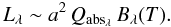 (1)The total luminosity of a dust population built from these grains is then given by
 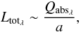 (2)if one uses the specific material density ρgrain, the number of grains n, and neglects any temperature dependency of Qabs. The scattering properties of dust grains are also affected (Mie 1908).
In addition to the changing optical properties of the dust grains, the grain sedimentation causes modification of the disc density structure. As a consequence, the spatial structure of the optical depth τλ changes, yielding different temperature profiles in the disc and re-emission features of the disc as a function of its evolving state. The altered optical depth structure also has implications for the morphology of scattered light images.
It is the goal of this study to investigate wether the dust grain growth and sedimentation-induced change in the disc structure can be observed. This will provide an ideal means of verifying current dust-coagulation models as well as allowing us to constrain the level of turbulence within circumstellar discs. However, the prediction and interpretation of observable quantities is rather complex. The optical properties of the dust together with the specific density distribution of the disc produce the highly non-linear behaviour of the respective observables including numerous ambiguities. Monte Carlo based codes have proven to be quite successful in the last decade in helping us cope with the complexity of the radiative transfer calculations on the model side. On the observation side, the careful interpretation of spectral energy distributions (SED) and images taken at different wavelengths provide insight into the nature of circumstellar discs.
In general, the SEDs of more evolved and settled discs have a smaller excess at longer wavelengths. This is paralleled by the common classification of classical T Tauri stars (CTTS) introduced by Lada & Wilking (1984). However, the Lada classification evaluates fluxes at wavelengths of 2.2 μm − 10 μm, while the flux decrease in the SEDs of settled discs occurs from the near-infrared (NIR) to millimetre wavelengths (e.g. Dullemond & Dominik 2005). Meeus et al. (2009) showed that the strength and shape of the 10 μm feature in T Tauri stars are related to grain growth. They also show that disc flaring and grain sizes are slightly related. D’Alessio et al. (2006) states that the essential effects of grain growth and dust sedimentation on the SED distribution of the disc can be summarised as follows:
-
more settled discs have a smaller far-infrared (FIR) excess;
-
more settled discs have lower midplane temperatures and consequently less flux in the millimetre regime;
-
discs seen edge-on display a lack of flux at intermediate wavelengths as a result of high optical depth at short wavelengths. A higher degree of sedimentation yields less extinction of the stellar light.
However, when fitting SEDs to observations, model parameters are often degenerate (e.g. Thamm et al. 1994; Boss & Yorke 1996; Schegerer et al. 2009). Furthermore, the SED is a spatially integrated observable of a disc. Hence, it can constrain them only very weakly as demonstrated by Robitaille et al. (2007).
The effects of dust settling on images of protoplanetary discs in the optical wavelength range are discussed by Dullemond & Dominik (2004). McCabe et al. (2003) report the first resolved image of an edge-on disc in the N band and demonstrate that at this wavelength the extent of the scattered light nebula is very sensitive to the grain size distribution. Experience gained from modelling individual discs has shown that multiwavelength, spatially resolved images are needed to allow us to constrain the disc density structure and dust grain properties (e.g. Wolf et al. 2003; Pinte et al. 2008; Sauter et al. 2009; Duchêne et al. 2010). While millimetre observations are sensitive only to radiation being emitted from dust in the densest region within the disc, NIR images are dominated by scattered stellar light from dust in the circumstellar envelope and the upper, optically thin disc layers. These observations trace different physical processes (scattering/re-emission) in different regions of the circumstellar environment, but they are both strongly related to the dust properties in the system. Watson et al. (2007) discuss the interpretation of images of multi-wavelength observations in detail. For example, the disc mass and the dust opacity cannot be distinguished as only their product is observable. Effects of parameters such as the disc dust mass or the inner and outer radii on images have been studied, by modelling both single objects and compilations (Pinte et al. 2008; Sauter et al. 2009; Brown et al. 2009; Sicilia-Aguilar et al. 2007). Stratified disc models with large dust grains close to the midplane and small grains in the upper layers and an envelope have been used to reproduce observations of several discs such as Duchêne et al. (2010), Sauter et al. (2009), Pinte et al. (2008), and Wolf et al. (2003). In these studies, a multiwavelength approach is used in order to constrain disc layers with different grain sizes. Distinct objects have been modelled with different dust models. For instance, some authors include graphite (Wolf et al. 2003) and some do not (Pinte et al. 2008). In the case of CB 26, this choice has implications for the maximum grain size (Sauter et al. 2009).
However, predictive studies analysing the impact of grain growth and sedimentation on observable quantities across a large wavelength range have so far only considered the effects on the SED (e.g. D’Alessio et al. 2006; Dullemond & Dominik 2004). As the next generation of telescopes and interferometers with high spatial resolution will commence in the not so distant future, it is vital to investigate whether and how grain growth and settling can be constrained by analysing spatially highly resolved images of circumstellar discs.
The present paper provides a first approach to addressing the need for a general investigation of the effects of dust grain growth and sedimentation on images from the near-infrared to the millimetre-regime. We identify indicators that allow the classification of observations and point out directions of interest that are worth a more detailed approach in subsequent studies. Addressed key questions are:
-
1.
what are the general effects of the grain-growth-induced massrelocation on images of a disc seen at different inclinations and atdifferent observing wavelengths?
-
2.
which tracers of dust grain growth and sedimentation are provided in general by edge-on millimetre images?
-
3.
what can be learned by combining mid-infrared images at various inclinations?
-
4.
how can grain growth and sedimentation be constrained by near-infrared images?
The present study will necessarily invoke several simplifications. Modelling of images of an individual object will provide a clearer insight into its particular evolutionary stage. Nevertheless, this study aims to provide a first, non-comprehensive guide into the field of imaging dust grain growth and sedimentation.
This paper is organised as follows. Section 2 introduces the model, the parameters, and the methodology employed. In Sect. 3, we illustrate the general effects of dust grain growth and sedimentation in images for a fiducial model. We also present tracers for grain growth and sedimentation in millimetre and mid-infrared images that are distinctive from other disc parameters. In Sect. 4, we discuss cases for which this fails.
2. Method
To investigate the effects of dust grain growth and sedimentation on observable quantities, four steps are needed. First, a model of a circumstellar disc has to be set up that includes the effects of dust settling and coagulation. Secondly, for all model parameters it has to be determined whether they should be set to some typical value or to be allowed to vary within a certain range. In the third step, radiative transfer simulations for every model have to be performed. As a concluding fourth step, the results of the radiative transfer simulations have to be investigated. In this section, we describe the first three steps.
2.1. The model
The basis of all our models is a parametrised disc density distribution. The dust density distribution ρdisc of such a disc can be written as ![Mathematical equation: \begin{equation} \rho_\disc(\vec{r})= \rho_0 \left( \frac{R_{100}}{\rcyl} \right)^\alpha \exp \left(-\frac{1}{2}\left[ \frac{z}{h}\right]^2 \right), \label{eqdiscden} \end{equation}](/articles/aa/full_html/2011/03/aa14546-10/aa14546-10-eq29.png) (3)where z is the usual axial coordinate with z = 0 corresponding to the disc midplane and rcyl is the radial distance from the z-axis. The quantity ρ0 is determined by the mass of the entire disc, R100 = 100AU is the radial normalisation constant, and h the local scale height
(3)where z is the usual axial coordinate with z = 0 corresponding to the disc midplane and rcyl is the radial distance from the z-axis. The quantity ρ0 is determined by the mass of the entire disc, R100 = 100AU is the radial normalisation constant, and h the local scale height 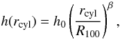 (4)where, α, β, and h0 in Eq. (4) are geometrical parameters. This disc model has served well already in describing observed discs, such as HH 30 (Wood et al. 2002), the Butterfly-Star IRAS 04302+2247 (Wolf et al. 2003), HK Tau (Stapelfeldt et al. 1998), IM Lupi (Pinte et al. 2008), HV Tau (Stapelfeldt et al. 2003), and CB 26 (Sauter et al. 2009).
To incorporate dust settling and coagulation, this ansatz has to be extended. A considerable amount of work has been done to understand the physics of dust grain coagulation and settling, including extensive numerical simulations on the topic, as well as dust coagulation studies in laboratories. A comprehensive treatment can be found in a series of papers by Blum et al. (2006), Langkowski et al. (2008), Weidling et al. (2009), and Güttler et al. (2009). Detailed models of dust grain growth and settling and the resulting vertical disc structure can be found in Dullemond & Dominik (2004). An analysis of the radial drift of dust grains can be found in Brauer et al. (2008) and Birnstiel et al. (2010). However, in the present work, we do not include the detailed picture of the dust growth process developed there. We use instead the parametrised ansatz that has been developed and successfully employed by D’Alessio et al. (2006).This enables us to formulate a parameter space that includes not only the basic parameters of the coagulation/sedimentation process but also important observational parameters that do not influence the disc physics but the way observations perceive them.
 |
Fig. 1 Sketch of the general model setup. Shown are the scale heights hsmall and hlarge of the two dust populations with |

To describe grain growth and settling, our model features two distinct dust populations that differ only in terms of the maximum grain size. For each population, the minimum grain size is the same as found in the ISM, amin = 5nm. The first population has the same maximum grain size as commonly assumed for the interstellar medium amax = 250nm (Mathis et al. 1977). This dust population is considered the reservoir of small dust grains from which the second population of larger grains is fed. The second component has a maximum grain size of 1mm. As described by Dullemond & Dominik (2004), the height to which a dust grain settles does not only depend on its size but also on the level of turbulence present in the disc. To model dust settling, both grain populations have different scale heights that are related via 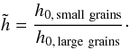 (5)Where h0,smallgrains and h0,largegrains are the respective scale heights. Figure 1 depicts the model concept.
In the initial state, both populations have the same dust-to-gas ratio. However, once the disc evolves towards the grown and settled case, the small dust grain population gets depleted and mass is transferred to the large dust grain population. The model of D’Alessio et al. (2006) parametrises the relative weighting of the two populations by the depletion parameter ϵ, which is the relation of the dust-to-gas ratio in the small grain population ζsmall to the default dust-to-gas ratio  given by
  (6)As neither accretion by the central star nor mass loss to the ambient space is considered, the dust-to-gas-ratio ζlarge of the large grain population has to be altered to keep ζ at its initial value. The values of ζlarge as a function of ζsmall are taken from D’Alessio et al. (2006). We also keep ϵ independent of the radial position in the disc.
2.2. The parameter space
Among its intrinsic parameters, our model features the observing wavelength and the disc inclination as external parameters. We now discuss their value and range.
2.2.1. Stellar heating
The stellar radiation heats the dust that then itself re-emits at longer wavelengths. We neglect accretion and turbulent processes within the disc as another possible intrinsic energy source. In this sense, the disc in our model is passive. We employ an “average” T Tauri star as given by the survey of Gullbring et al. (1998). This star has a radius of r = 2R⊙ and an effective surface temperature of Teff = 4000K. Assuming the star to be a black-body radiator, this yields a luminosity of L ∗ = 0.92 L⊙.
2.2.2. Dust properties
We assume that the gas within the disc is optically thin and limit ourselves to radiative transfer through the dust and neglect line emission and absorption by the gas. This is justified as the dust is the dominant coolant of the disc. Hence, thermal equilibrium obtained in radiative transfer calculations based on dust only will provide a reliable description of the disc’s thermal structure. This assumption is based on the work of Kamp & Dullemond (2004), who showed that dust and gas temperature in a circumstellar disk around a T Tauri star are well coupled in the regions that are sufficiently dense to be traced with current and near-future (sub)millimetre observatories.
We assume the dust grains to be homogeneous spheres. Real dust grains are expected to have a far more complex and fractal structure. As discussed by Voshchinnikov (2002), chemical composition, size, and shape of dust grains cannot be determined separately, but only as a combination.
We keep the dust composition of silicate graphite material fixed to avoid degeneracies. For the optical data, we use the complex refractive indices of “smoothed astronomical silicate” and graphite as published by Weingartner & Draine (2001). For graphite, we adopt the common “ ” approximation. As shown by Draine & Malhotra (1993), this graphite model is sufficient for extinction curve modelling. Applying an abundance ratio of silicate to graphite of 1 × 10-27 cm3H-1: 1.69 × 10⁻²⁷ cm3H-1, we get relative abundances of 62.5% for astronomical silicate and 37.5% graphite (
 and
and  ).
).
As the grain size distribution, we assume a power law of the form  (7)Where, a is the dust grain radius and n(a) the number of dust grains of a specific radius. For each dust grain ensemble, 1000 logarithmically and equidistantly distributed grain sizes within the interval [ amin:amax ] were taken into account. For simplicity reasons, we assume Eq. (7) to be valid in the whole disc for each grain population individually. Kim et al. (1994) argued that to achieve a good fit to U, B, and V linear polarisation measurements, the grain size distribution has to depart from the power law. However, the grain size distribution in a specific region of the circumstellar disc depends on the grain evolution there, which depends on a variety of factors. First, grains are understood to grow fast in the denser regions of the disc. Secondly, mixing and fragmentation processes will also influence the grain size distribution. With the model employed in this paper utilising two different grain populations, we consider the effects of the vertical dust grain settling. The overall grain size distribution then deviates accordingly from a simple power law. Finally, we assume an average grain mass density of ρgrain = 2.5gcm-3.
2.2.3. Parametrisation of growth and settling: ϵ and 
In the framework of our model, we follow the parametric values given by D’Alessio et al. (2006) for the depletion parameter ϵ and the relative sedimentation height  . For coagulation and settling induced deviations from the default mass-to-gas relation of the small grain population, we have ϵ = 1.0, 0.1, 0.01, and 0.001. The quantity describes the level of turbulence in the disc. As this level is generally not known, we adopt three values for
  , scattered around the D’Alessio et al. (2006) value of 10, i. e. we have
  , 12, and 20.
2.2.4. Disc flaring and surface density
In our model (Eq. (3)), two exponents α and β control the density distribution of the disc. The exponent p of the surface density Σ = Σ0rp is directly related to α and β via p = α − β.
Most observed circumstellar discs can be described well by a relatively small range of values for α and β. Good agreement between model and observations are found for values of  and α according to the relation
  , which is a result of viscous accretion theory (Shakura & Sunyaev 1973). Thus, these two parameters are also kept fixed in order to reduce the free parameters of the model. We employ the values obtained for the Butterfly star (Wolf et al. 2003): α = 2.37 and β = 1.29.
2.2.5. Inner and outer radial extent of the circumstellar disc
Earlier and recent modelling efforts have shown a variety of size scales of the inner disc radius. Some discs are most accurately described using an inner radius as small as the sublimation radius for silicate at T = 1500K. This temperature is reached at a distance of about 0.07AU from the T Tauri star in our model. An example of this configuration can be found in Wolf et al. (2003). Other discs, such as HH 30 (Guilloteau et al. 2008), apparently have a large inner void with radii up to ~ 45AU from the star. To incorporate both types of discs, we allow the inner radius to have the values rinner = 0.1AU, 1.0AU, and 10AU.
The outer radius of the dust disc is also subject to variation. For discs around T Tauri stars, disc radii vary from 25AU (Neuhäuser et al. 2009) to 400AU (Simon et al. 2000). Hence, we allow in our study the outer disc radius to have the values router = 100AU, 300AU, and 400AU.
2.2.6. The total disc dust mass
The values for the total dust mass of the disc span a range of three orders of magnitude: mdust = 3.2 × 10⁻⁶M⊙, 3.2 × 10⁻⁵M⊙, and 3.2 × 10⁻⁴M⊙.
2.2.7. Choices of inclination
The inclination under which a circumstellar disc is observed is a non-intrinsic quantity of the model. In the case of face-on discs (θ = 0°), one has direct observational access to the central star, while in the edge-on case the star is typically completely obscured by the dust disc. On the other hand, the edge-on case might allow us to examine the vertical structure better if upper disc layers are sufficiently transparent. It is one goal of this study, to determine the extent to which the vertical disc structure can be determined by observations. We include both extrema in our study.
2.2.8. Observing wavelengths
To predict observational quantities in a multiwavelength set-up, we compute images in the near-infrared, mid-infrared, and sub-millimetre and millimetre regime. Altogether, this gives us images in the I, J, H, K, L, M, N, and Q band (central wavelength λ = 1.0 μm,1.25 μm,1.6 μm,2.2 μm,3.4 μm, 4.7 μm, λ = 10 μm, and 20μm) as well as 15 μm, 50μm, 100μm, 350μm, 670μm, 840μm, 1100μm, and 1300μm. For computations of observed fluxes, a distance of 140 pc is assumed, which is representative of the well-studied low-mass star-forming region in the Taurus constellation.
2.3. Radiative transfer simulations
For the continuum radiative-transfer simulations, we use the program MC3D1 (Wolf et al. 1999; Wolf 2003) which is based on the Monte Carlo method and solves the continuum radiative-transfer problem self-consistently. The program uses the temperature correction technique described by Bjorkman & Wood (2001), the absorption concept introduced by Lucy (1999), and the enforced scattering scheme proposed by Cashwell & Everett (1959). Multiple and anisotropic scattering is considered. The radiative transfer is simulated at 100 wavelengths, logarithmically distributed in the wavelength range [ λmin,λmax ] = [ 50nm,2.0mm ] .
2.4. Beyond the model
Our model setup is based on several simplifications. The shape of the disc, governed by α and β in Eqs. (3) and (4) is kept fixed. The flaring of the disc surface given by β has a significant influence on the amount of intercepted stellar radiation, hence the thermal structure of the disc, as well as the spatial distribution of scattered light. As discussed by Watson et al. (2007), these two parameters also have an impact on the width of the dark lane in a way similar to depletion parameter ϵ (see Sect. 3.1). The freedom to vary α and β harbours a degeneracy in this respect. Nevertheless, this is not necessarily a drawback. To understand the influence of all possible physical processes, careful investigation of each is needed separately. To do this for the effects of sedimentation on images in the described framework is the goal of this paper.
3. Results
We investigate for the parameter space of our model the effects on various observational quantities that allow one to constrain dust settling and coagulation. In particular, we examine the implications of the depletion parameter ϵ and the scale height relation in Sect. 3.1. The general result is that dust settling and coagulation described by the depletion parameter ϵ can be constrained by various observations if the disc is seen edge-on. The respective findings are presented in Sects. 3.2 and 3.3. The possible ways to constrain the relative scale height (i.e. the amount of turbulence in the disc) is discussed in Sect. 3.4. These findings hold true only in the parameter space outlined in Sect. 2, especially the exact value of modelled fluxes or the morphology of images, particularly in the mid-infrared. Nevertheless, the qualitative behaviour of tracers for grain growth and sedimentation outlined in this Section can also be expected for models with, for instance, different choices of α, β, or h0 in the density distribution (cf. Eq. (3)).
3.1. The fiducial model
To discuss the effects of dust grain growth and coagulation on observable quantities and as a reference for future investigations, we introduce a fiducial model. Its parameters are rinner = 0.1AU, router = 300AU, mdust = 3.2 × 10⁻⁴M⊙, , and ϵ = 1.0. This approach allows us to evaluate the impact of variations in the individual model parameters on the observable quantities. The resulting degeneracies are discussed.
3.1.1. Effects of the depletion parameter ϵ
The depletion parameter ϵ governs how much mass is transferred from the small to the large dust grain population. Therefore, ϵ can be understood as a parameter for dust grain coagulation and the resulting sedimentation.
The near-infrared images of edge-on discs exhibit a pronounced chromaticity. In this wavelength regime, the disc’s midplane is optically thick and shields the central star from direct observation. The height above the midplane at which the disc becomes transparent to the scattered stellar light constrains the disc’s scale height.
Besides the optical properties of the dust particles, the opacity of the disc depends on the amount of dust from both dust populations present in the respective disc layers. Considering dust settling, the composition of these layers is a function of the degree of depletion. Thus, the width of the dark lane is not a function of the disc gas scale height alone but must also be a function the depletion parameter ϵ. The fiducial model exhibits this behaviour. Figure 2 shows both the dependence of the dark lane on the observing wavelength λ as well as the depletion parameter ϵ. Although the values for λ and ϵ in the plot do not exactly mirror each other, the width of the dark lane can be reproduced by adjusting both parameters.
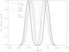 |
Fig. 2 Dependence of the width of the dark lane in scattered light images on the depletion parameter ϵ (grey) and the observing wavelength λ (black). Shown are cuts through images along the disc midplane centred on the projected position of the embedded star. |
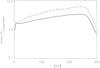 |
Fig. 3 Selected flux ratios of the radial brightness profile of the fiducial model seen in the H band face-on. The solid line shows the flux ratio of models with ϵ = 1.0 to ϵ = 0.001. The dashed line shows the ratio of fiducial models with mdust = 3.2 × 10⁻⁴M⊙ to mdust = 3.2 × 10⁻⁶M⊙. |
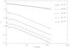 |
Fig. 4 Optical depth of the fiducial model along radial paths for selected inclinations as a function of wavelength. A high optical depth in the millimetre regime is obtained only for high inclinations, while for shorter wavelengths the model is opaque in a wider range. |
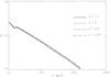 |
Fig. 5 Optical depth of the fiducial model along a radial path at 90° inclination as a function of wavelength. Only a weak dependence on the depletion parameter ϵ exists. |
Figure 3 shows the relation of the radial brightness profile of the fiducial model with different total dust masses and different depletion parameters ϵ observed face-on. For r = 0, the ratio of the fluxes of the fiducial model with ϵ = 1.0 to ϵ = 0.001 is 1 since the same stellar properties are used for all models. For r > 0, the ratio of the brightness profiles is ≈ 2 for different depletion parameters ϵ, while it is slightly sloped for different total dust masses. A variation in the density structure (i.e. α and β in Eq. (3)) can easily counterbalance the effects shown in the plot. For inclinations θ = 60° and θ = 0°, the dependence of the brightness distribution on ϵ is almost lost.
The first reason for this ambiguity is that as the disc is tilted to smaller inclinations, the dark lane vanishes. This is because the optical depth along the line of sight decreases and more scattered stellar light reaches the observer.
Secondly, as the disc itself is still optically thick in the near infrared, it is still only the upper disc layers that are penetrated by stellar light. Hence, it is the same physical environment as in the edge-on case that determines the characteristics of the scattered light.
Figure 4 shows the dependence of the optical depth as a function of the wavelength for selected radial paths. A high optical depth (τλ ≫ 1) in the millimetre regime is obtained only at high inclinations. For shorter wavelengths, especially in the near-infrared, the fiducial model is opaque even for θ ~ 70°. Figures 5 and 6 show the dependence of τλ along a radial path on the depletion parameter ϵ. For the edge-on orientation θ = 90°, the dependence τλ(ϵ) is very weak (Fig. 5). Nevertheless, 5° away from the edge-on orientation, the optical depth is far more sensitive to the depletion parameter ϵ (Fig. 6).
For images taken in the sub-millimetre and millimetre regime, no distinctive effect is observed. While absolute flux values change as the large dust grain population becomes more massive, no relative effect is seen either with respect to the location within one image or as a function of wavelength. These findings hold true for any inclination we considered in our framework. Since for smaller values of ϵ, more large grains are present in the system and large grains re-emit more efficiently at longer wavelengths than smaller grains do, one might expect observable effects in the millimetre regime. For the case of an edge-on disc the results are discussed in Sect. 3.2. However, if the disc is seen face-on, there are no observable effects.
3.1.2. Effects of the height relation 
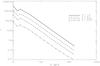 |
Fig. 6 Optical depth of the fiducial model along a radial path at 85° inclination as a function of wavelength. Unlike the situation in the exact edge-on case (Fig. 5), the optical depth becomes sensitive to the depletion parameter ϵ by typically half an order of magnitude. |
The height relation as defined in Eq. (5) describes the level of turbulence in the disc as well as the magnitude of the viscosity parameter α.
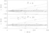 |
Fig. 7 Contour lines of the density distribution normalised to the respective peak density of the two grain populations. The two panels show the effect of small (top) and large (bottom) relative scale height |
Figure 7 illustrates the effects of on the density distribution. The density distribution of the small grain population does not depend on . According to the model set-up, the large grain population becomes concentrated in a much smaller space for larger .
The effects of on images at different inclinations is essentially that of an amplifier of effects caused by the depletion parameter ϵ. For near-infrared images of edge-on discs, the width of the dark, high-opacity lane is affected. Larger values for the height relation result in a dark lane with larger contrast and vice versa. This can be readily understood in terms of optical depth. Higher values of essentially squeezes the large dust grain population into a smaller volume and thus increases the optical depth. The amplifying effect is stronger for smaller values of ϵ: more mass is packed into the large dust grain population yielding a height optical depth.
The magnitude of the effects caused by the variation in is considerably small. In Fig. 8, the optical depth of the fiducial model along a radial path in the edge-on orientation as a function of wavelength is shown. The comparison with Figs. 5 and 6 shows that for the dependence is not as strong as for ϵ.
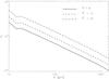 |
Fig. 8 Optical depth of the fiducial model along a radial path at 90° inclination as a function of wavelength. Plotted is the dependence on the relative scale height |
3.2. Millimetre images
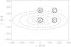 |
Fig. 9 Location of the four regions used to compare intensities. The dashed lines are logarithmic contour lines of the brightness distribution of the fiducial model observed at λ = 1.3mm and θ = 60°. |
Millimetre images are well suited to classifying dust settling and coagulation because at these wavelengths the dominant fraction of the radiation has its origin in the thermal re-emission of the dust grains. Furthermore, the redistribution of the mass also alters the optical depth structure. The most illustrative way of seeing how millimetre images can help us constrain disc evolution (the changing radial and vertical opacity and thus the reemission structure) is to compare different regions of a disc image, especially if the disc is seen edge-on. The regions of our choice are depicted in Fig. 9 and labelled (cw, starting in the image/disc centre) A, B, C, and D. One expects that as the disc evolves, the layers more distant from the midplane lose increasingly more mass because of the dust grain growth and settling towards the midplane, the amount of thermal re-emission from those layers also decreases. Radiation originating close to the midplane is expected to rise or stay at the same level, since the growing midplane mass not only yields more emitting grains but also more absorbing grains (important in the submillimeter regime). Densities are already orders of magnitude higher close to the disc midplane, the down-raining grains thus being unable significantly increase the optical depth and produce any gain in emitter numbers.
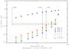 |
Fig. 10 Analysis of image brightness distribution of a circumstellar disk at different evolutionary stages. The results for different evolutionary states are coded in colour. The shape of any mark denotes the region from whence it is taken. Vertical lines indicate resolution limits of selected interferometers. Horizontal lines give the ALMA sensitivity limit, the other two instruments do not have the required sensitivity. The flux is given in units of the total flux. Since this flux depends as well on ϵ, the sensitivity limit is affected. The dependence of the flux in regions B and C on ϵ is shown. |
Figure 10 shows our findings exemplarily by relating the flux from the four different regions to the total flux, starting from red for the early ϵ = 1.0 case and ending at blue with a depletion parameter ϵ = 0.001. The shape of any mark denotes the region from whence it is taken. We plot the relative flux from a certain region versus the size of that region. The latter can be understood as the degree of resolution of the observing instruments. As an indicator, the maximum resolution at 1.3 mm of various instruments (ALMA, PdBI, SMA) is given as dashed black lines. Although all three interferometers shown in the plot provide the required resolution to detect the effect, only ALMA provides the required sensitivity. As the flux is given in units of the total flux of the image, which depends on ϵ, the sensitivity is also a function of ϵ. As expected, fluxes taken in the midplane do not vary considerably with the evolutionary state: all four colours are almost on top of each other. However, for fluxes taken from above the disc midplane, a clear decrease in flux is visible. From the initial ϵ = 1.0 to the final ϵ = 0.001, it spans almost two orders of magnitude.
This effect of the flux decrease though is limited to the edge-on case only. At inclinations of θ = 60°,0°, the lines of sight are no longer within the midplane or any parallel plane but intersect higher disc layers as well as the disc midplane. As a result, the radiation comes from various disc layers, representing different stages of dust coagulation and sedimentation. The amount of flux collected in the four different regions is not a function anymore of the depletion but only of the disc’s geometrical thickness. As the inclination can be determined from imagemorphology, these findings are a valuable tracer for dust sedimentation in the edge-on case.
To estimate the robustness of this result, we consider the influence of disc parameters other than the depletion factor ϵ. We find that although the total flux value from different regions changes, the effect of the separation between the flux values in the upper and lower layers of the image with later evolutionary states does not depend on the chosen parameter value. It is also independent of the observing wavelength in the (sub) millimetre regime.
3.3. The disc in N and Q band edge-on
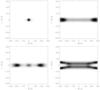 |
Fig. 11 Different morphologies of an edge-on disc in the N band with rinner = 0.1AU. Top left: mdust = 3.2 × 10⁻⁶, router = 300AU, |

We now turn our attention towards the potential of mid-infrared observations in the N and Q bands. In our chosen models, the re-emission in these bands dominates the scattered stellar flux by several orders of magnitude. Morphologically, it is the transition region from the “dark lane” type of brightness distribution, as seen in the near-infrared (see Sect. 4.2), to the extended and elongated shapes typical of objects in (sub)millimetre images. In our edge-on images, the typical central dark lane is very thin, of the order of one resolution element of the Giant Magellan Telescope. The major difference from millimetre images of edge-on discs is that the flux due to re-emission is concentrated in the central region, while at increasing wavelength the emission becomes increasingly extended as cooler material dominates the emission.
On the basis of our model, we predict the various morphologies that can be observed in this wavelength regime. The possibilities for our parameter range include a single central peak, two elongated emission regions separated by a dark lane, three emission maxima in the midplane, a four-legged x-like shape, and others more. Figure 11 gives an impression of the variety of possibilities. The reason for this broad range of different morphologies is the fine-tuning of the optical depth. Depending on the total mass and its distribution, different regions of the disc for a specific choice of parameter values are rendered opaque enough such that their radiation contributes (or not) to an image. In most cases, τλ is close to unity to within an order of magnitude.
However, the overall width of the brightness distribution turns out to be a valuable tracer of dust grain growth and sedimentation in the edge-on case (see Fig. 12). A linear relation between the full width at half maximum (FWHM) of the emission regions in the two bands is observed. For all possible combinations of parameters in our framework, the scattering of the Q band peak width versus the N band peak width is strongest for a large depletion parameter and ceases for later evolutionary stages.
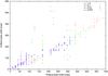 |
Fig. 12 FWHM of the height of the emission in N band versus the same in Q band for different values of the depletion parameter ϵ. A general tendency of a linear relation between the FWHMs for smaller values of ϵ can be observed. |
Linear slope and  of the N/Q band width of the models.
Introducing a straight line as a fit, the chi-square () is a function of the depletion parameter ϵ as shown in Table 1. The reason for this increasing linearity between the FWHM of the emissions in the two bands is the fine-tuning of the optical depth. Re-emitted radiation received from the object originates at regions with an optical depth smaller than unity. For large values of ϵ, the disc dust mass is distributed over a larger volume. Thus, the iso-surface with τNband has more morphological freedom. Consequently, the width of the brightness distribution of one disc model picked at random depends more on the setting of the other parameters than this is the case for smaller values of ϵ. There the bulk of matter is concentrated close to the midplane and the shape of the regions seen is less sensitive to a specific choice of parameters, i.e. the density distribution of the large grain population determines the width of the brightness distribution alone, not the interplay between two grain populations.
The specific value of the slope in Table 1 is roughly determined by the wavelength dependence of τ and the vertical density increase in the large dust grain population as given by Eq. (3). Increasing the observing wavelength from 10 μm to 20 μm allows a deeper look into regions of higher disc densities. For ϵ = 0.001, a slope of 0.8 implies that the Q band image is a little thinner than the N band image. This means that the spatial gain by reduced optical depth is almost counterbalanced by the higher density in deeper layers.
Within our parameter space, the FWHM-relation of the emission thickness in N and Q band for one disc depends on the total dust mass. An analysis of disc models shows that they group in Fig. 12 according to their total dust mass, not their relative scale height. This is also true for later evolutionary stages.
Consequently, the evolutionary stage of a single observed disc can be inferred by comparing the extent of the emission in the N and Q band only. The precise value of this relation will depend on the global geometry of the disc. Nevertheless, a peak width ratio of ~ 0.8 from Q to N band is a good indicator for discs in which most of the mass settled as large dust grains close to the midplane.
3.4. Q and N band face-on: turbulence digs in
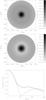 |
Fig. 13 Face-on images in the N band and radial profiles of the brightness distribution. Top: fiducial model with a scale height relation of |

This section is dedicated to investigating if the relative scale height can be constrained. Figure 11 already indicates that images in the N and Q band are sensitive to the fine-tuning of the density distribution. Figure 13 illustrates this in the N band for the case of face-on discs. In this regime, the observed flux originates predominantly from re-emission of hot dust at ~300K.
The marker for the relative scale height is the gap in the flux distribution at intermediate disc radii of ~100 AU. The strength of this emission gap depends directly on the relative scale height . For large , hence small scale-height of the large dust-grain population, the gap is clearly visible, but is non-existent for smaller values of . The effect also depends on the observing wavelength.
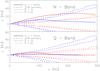 |
Fig. 14 Temperature distribution and isolines of constant optical depth τ = 1 in the N band (top) and Q band (bottom) for the fiducial model. Different colours refer to different relative scale heights |
The nature of this apparent gap can be understood by analysing the spatial temperature distribution together with the optical depth. Figure 14 shows temperature contour lines of the large-grain population enclosing regions with temperatures higher than the black-body emission peak in the Q and N band. This emission peak occurs for the Q band at 144 K and the N band at 315 K. Regions outside are cooler. Closer to the midplane the reason for this is the high optical depth such that the material there cannot be heated effectively by stellar radiation. Far above the midplane the density of the disc is too low to assign a meaningful temperature (cf. Fig. 7). Figure 14 also shows the τQ,N = 1 isoline for the two bands obtained by integrating perpendicular to the midplane, starting at z = ∞. For both bands and the two extreme values for , the high temperature regions of the small grain population are far above the τQ,N = 1 line and are not shown in the plot. In both bands, these regions most efficiently contribute to the face-on image of the disc for any value of . These regions are the origin of the flux peak in the centre, cf. Fig. 13.
In the Q band, the large-grain population also contributes to the image for both values of . Unconvolved face-on images show that the surface brightness of the small-grain population is about an order of magnitude larger. The emission region of the small grain population is close to the rotation axis of the system. Seen from above, all emission of the small grain population is seen piling up in a narrow region, while the emission regions of the large grain population are stretched above the midplane. In the edge-on case, this geometrical effect yields the opposite result: the emission from the large grain population is seen in a smaller area and thus contributes more to the image than the small grain population.
Matters are different in the N band. An optical depth of τN = 1 is reached at higher altitudes from the midplane than in the Q band. For  and small radii, the emitting region is below the τQ = 1 isoline. This leads to a fainter emission in the N band from intermediate causing the brightness gap at these radii.
The isolines indicate how deeply face-on observations can penetrate into the disc. Wien’s law only allows us to determine the grains and disc layers that emit most efficiently in a given wavelength band (e.g. Schegerer et al. 2006). Many more grains of either lower or higher temperature can also explain the dominating flux at the wavelengths in question. However, in Fig. 14 all regions with higher temperatures are included by the temperature contour lines. Since the emitted energy is proportional to ~ T4, the reasoning in the previous paragraph remains robust.
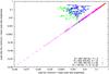 |
Fig. 15 Classification of the apparent gap in the brightness distribution of edge-on seen in the N band. We show the total brightness minimum in units of the average disc brightness in the outer |

Figure 15 shows that the contrast of the brightness gap is a function of the relative scale height for two thirds of our parameter space. We plot in units of the average disc brightness in the outer third of the disc the total brightness minimum versus the minimum brightness in the outer third of the disc also in units of the average outer disc brightness. Models featuring a gap have a flux minimum within the first two thirds of the disc and are located left of the line of unity slope. Models without an inner gap appear on the line of unity slope. The gap is typically located at radii r ≈ 100AU, and discs with an outer disc radius of router = 100AU consequently do not exhibit a gap. In Fig. 15, these discs are all located on the line of unity slope.
We define the width of the gap as the radial distance between the location of the first brightness maximum after the gap and the location where the brightness distribution close to the centre reaches the maximum value. Figure 16 shows the minimum flux in the gap as a function of this gap width. Models with very pronounced gaps are thus located in the lower right part of the plot. Models with different values of are also shown. The strength of the gap does not correlate with as can be seen from Fig. 16, but the width of the gap does. Our analysis also indicates that the gap width does not correlate with the outer disc radius router.
4. Other markers: Discussion
Our study also shows, that markers other than those presented in Sect. 3 are insufficient to constrain grain growth and coagulation. However, we discuss them in this section to shed further light on the nature of the images of circumstellar discs.
4.1. Radial profiles in the millimetre regime at low inclinations
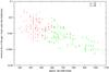 |
Fig. 16 Classification of the brightness gap of face-on seen discs at λ = 10 μm. On a log-linear scale, we plot the total brightness minimum in units of the average disc brightness in the outer third of the disc versus the gap width. Models are colour coded with different scale height relation |

The observed flux in (sub-)millimetre images stems from dust grain re-emission at these long wavelengths. The optical depth is small rendering all dust particles visible. As our models are rotationally symmetric, it suffices to consider the radial brightness profile instead of the whole image. However, these profiles do not provide means by which discs at different stages of their evolution can be distinguished. While the absolute value of the radial profile of the surface brightness distribution depends on the evolutionary stage of the disc, the shape of the profile does not. This renders the radial profile for θ < 90° degenerate with respect to mdust and ϵ. This behaviour agrees with the findings of Sect. 3.2.
4.2. Dust lane chromaticity in the near-infrared
In the near-infrared, the typical appearance of a circumstellar disc seen edge-on is a bipolar structure that is intersected by a dark lane. The width of the dark lane is an effect of optical depth and wavelength dependent. In addition, at wavelengths between 2 μm and 10 μm, the radiation due to the thermal re-emission of dust grains is increasingly more important in our disc models than scattered stellar radiation. In the mid-infrared, the re-emitted radiation is by far the dominant contributor to the total flux.
Since the optical depth is a function of the disc mass, one expects the width of the dark lane to be dependent also on the depletion of the upper disc layers. As the grains grow in size and rain down towards the midplane, the upper layers become less opaque and might affect the width of the dark lane as an indicator for ϵ. Increasing the observing wavelength unveils deeper layers in the disc and the large dust-grain population (cf. Fig. 7) increasingly influences the appearance of the disk.
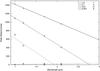 |
Fig. 17 The chromaticity and dependence of the width of the dark lane on the depletion of upper disk layers in the NIR wavelength regime. For longer wavelengths and smaller ϵ the width is generally smaller. We also shown the straight-line fits. |
Figure 17 shows the width of the dark lane for the fiducial model. As expected, the width of the dark lane decreases with both wavelength and increasing depletion of the upper disc layers. The chromaticity itself is a function of ϵ (otherwise the fitted lines would be parallel). For smaller ϵ, the chromaticity of the dark lane is less steep. Moreover, the chromaticity’s dependence on ϵ provides a means of identifing dust grain growth and settling uniquely via near- to mid-infrared imaging only. In Fig. 18, all chromaticity slopes mϵ for all possible parameter combinations within our framework are given. For any given ϵ, the slope obtained is either zero or scatters within a certain range. The depletion of the upper disc layers could be inferred from the slope if a unique relation between ϵ and the chromaticity slope were observed, which is not the case.
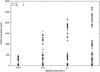 |
Fig. 18 Scatter plot of the chromaticity-slope of the dark lane for different ϵ and different fit ranges. |
The same behaviour is observed when not only images in the I, J, H, and K bands but also the L and M bands are considered. These two bands mark the transition region between images dominated by scattered stellar light and dust grain re-emission. This is independent of the resolution used to image a given circumstellar disc in the NIR.
4.3. Near-infrared and millimetre images
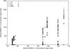 |
Fig. 19 Width of the dark lane as a function of the FWHM of the millimetre emission. Colour coded is the depletion parameter ϵ. A clear dependence of ϵ on the width of both is not seen. |
One might expect that a combination of millimetre and near-infrared images should provide insight into dust grain growth and sedimentation in a similar way to the combination of images in the N and Q. Figure 19 gives the relation between the FWHM of the vertical extend of the spatial brightness distribution in the millimetre regime and the width of the dark lane in the J band. The high dust densities in the disc mid-plane are responsible for the dark lane in the NIR and the elongated spatial brightness distribution in the millimetre regime. Thus, a relation between the width of the dark lane and the millimetre emission region provides an indicator of to the disc’s evolution. However, as Fig. 19 shows, no correlation between the two quantities is observable.
4.4. Degeneracy between parameters and panchromatic studies
We point out that if all disc parameters in our parameter-space are known, in most cases the chromaticity of the dark lane uniquely determines the evolutionary state, as illustrated by the fiducial model (cf. Sect. 3.1). In general, it is impossible, however, to determine the evolutionary stage of a disc when other parameter values also remain unconstrained. As a simple counter-example, consider a system that is optically thin at all near-infrared wavelengths, for which a dark lane is thus not visible and no chromaticity can be seen. In our model framework, this happens for discs with either a low total dust mass, a low scale height relation , a high depletion parameter ϵ, or a combination of both. The total dust mass can be constrained by the systems’ total flux in the millimetre regime where the disc is generally optically thin. However, to constrain a certain total dust mass is required. The effects of are rendered indistinguishable otherwise.
4.5. The general face-on case
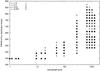 |
Fig. 20 The FWHM of the spatial intensity distribution of disc observed face-on as a function of wavelength. The depletion parameter ϵ is encoded with different symbols. |
As shown for millimetre images in Sect. 3.2, the ability to constrain dust sedimentation by single imaging is lost for θ < 90°. For images in the near-infrared and mid-infrared the situation is similar. In Fig. 20, we present plots of the FWHM of the disc’s brightness distribution seen edge-on at different wavelengths. At relatively short wavelengths, the emission is very small because in the NIR the star is the dominant contributor to the image flux. Images have an apparently broader flux distribution at longer wavelengths since the origin of the observed flux changes from scattering to re-emission. The size of the re-emission region increases as the observing wavelengths get longer and cooler parts provide more important flux contributions. In Fig. 12, we can discern a grouping of data points with smaller ϵ close to a linear relation between the N and Q band emission width, no such relation is seen in a NIR/millimetre comparison. Even if a parameter is well constrained by some observation no specific behaviour of data points with the same depletion parameter ϵ can be seen.
This observation does not contradict the findings of Dullemond & Dominik (2004). In their work, dust grain growth and sedimentation have not been modelled with a parametrised model but including radius-dependent sedimentation. In our model framework, we do not allow for radial-dependent dust settling. More rapid dust-grain growth at smaller radii renders the upper disc layers in the inner disc more transparent and allows the stellar radiation to heat the outer disc more efficiently. The radial brightness profile would then spread outward. In contrast, the upper layers all lose mass at the same rate in our framework. Hence the radial brightness profile is unaltered.
The last result is only true for the relative profile, that is a profile normalised to some other disc inherent quantity. For most practical cases this would be the total disc flux. The absolute flux values change with the evolution of the disc (cf. Sect. 4.1).
5. Conclusions
We have explored the effects of dust grain growth and sedimentation on images of circumstellar discs at various wavelengths and inclinations. As the prediction of observable quantities of circumstellar discs is highly non-linear and harbours several degenerate parameters, we have employed a simplified, parametrised model. This has allowed us to discuss the general effects of the depletion of upper disc layers by grain growth and dust sedimentation using radiative transfer simulations in the near-infrared, the mid-infrared, as well as the (sub-)millimetre regime. In the advent of telescopes providing high spatial resolution, we have focused on images at these wavelengths thus extending existing studies on SEDs. Although our approach is based on certain simplifications, we have identified tracers that uniquely allow us to constrain the evolutionary stage of a disc.
In particular, our findings have direct implications for future observations:
-
The width of the dark lane in NIR images of edge-on discs isdegenerate with respect to the degree of depletion of upper disclayers from large grains and observing wavelength. Althoughthis wavelength and the degree of depletion do not exactly mirroreach others impact on the width of the dark lane, a given width lanecan be reproduced by adjusting both parameters (seeSect. 3.1).
-
High spatial resolution also needs to be accompanied by high sensitivity in the case of millimetre images. Only ALMA will provide the required resolution and sensitivity to identify grain sedimentation in millimetre images of edge-on seen discs. A settled disc exhibit a relative surface brightness decrease of ~ 10-4 from the mid-plane to 150 AU above the disc, while non-settled discs display a decrease of only ~ 10-2 (see Sect. 3.2).
-
If the disc is not seen edge-on, then this distinction between settled discs and non-settled discs cannot achieved by millimetre observations, if the settling is independent of the radial position in the disc.
-
A comparison of the FWHM of the brightness distribution in N and Q band images allows us to constrain the degree of dust sedimentation in a circumstellar disc if seen edge-on. Evolved discs in our parameter space have a ratio of the Q band FWHM to the N band FWHM of ~ 0.8 that depends only very weakly on other disc properties. Young discs however show a ratio that depends strongly on other disc parameters and exhibit significant scatter for various combinations of parameter values around the average FWHM ratio of ~ 1.0 (see Sect. 3.3).
-
The relative sedimentation height
to which particles settle can be determined using face-on observations in the N and Q band. Owing to the complex interaction between the spatial structure of the optical depth and the temperature distribution, discs in which large grains settle close to the mid plane exhibit a gap in the observed radial brightness distribution at typically ~ 100AU. However, the effect is only seen in discs considerably larger than ~ 100AU (see Sect. 3.4).
Furthermore, we discuss ambiguities that prevent us achieving the same results for images in other wavelength regimes, namely the near-infrared.
As a next step, a disc parametrisation should be chosen that allows us to incorporate radially dependent sedimentation. Modelling images of an individual object will provide additional insight into its particular evolutionary stage. The knowledge gained in the framework of the present paper forms a non-comprehensive basis for further analysis of dust grain growth and sedimentation effects on images.
Available upon request: This email address is being protected from spambots. You need JavaScript enabled to view it. .
Acknowledgments
J.S. thanks C. Dullemond for enlightening discussions. J.S. acknowledges support by the DFG through the research group 759 “The Formation of Planets: The Critical First Growth Phase”.
References
- Beckwith, S. V. W., & Sargent, A. I. 1991, ApJ, 381, 250 [NASA ADS] [CrossRef] [Google Scholar]
- Birnstiel, T., Dullemond, C. P., & Brauer, F. 2010, ArXiv e-prints [Google Scholar]
- Bjorkman, J. E., & Wood, K. 2001, ApJ, 554, 615 [NASA ADS] [CrossRef] [Google Scholar]
- Blum, J., Schräpler, R., Davidsson, B. J. R., & Trigo-Rodríguez, J. M. 2006, ApJ, 652, 1768 [NASA ADS] [CrossRef] [Google Scholar]
- Boss, A. P., & Yorke, H. W. 1996, ApJ, 469, 366 [NASA ADS] [CrossRef] [Google Scholar]
- Brauer, F., Dullemond, C. P., & Henning, T. 2008, A&A, 480, 859 [NASA ADS] [CrossRef] [EDP Sciences] [Google Scholar]
- Brown, J. M., Blake, G. A., Qi, C., et al. 2009, ApJ, 704, 496 [NASA ADS] [CrossRef] [Google Scholar]
- Cashwell, E. d., & Everett, C. J. 1959, A practical manual on the Monte Carlo Method for random walk problems (Pergamon) [Google Scholar]
- Cuzzi, J. N., Dobrovolskis, A. R., & Champney, J. M. 1993, Icarus, 106, 102 [NASA ADS] [CrossRef] [Google Scholar]
- D’Alessio, P., Calvet, N., Hartmann, L., Franco-Hernández, R., & Servín, H. 2006, ApJ, 638, 314 [NASA ADS] [CrossRef] [Google Scholar]
- Draine, B. T., & Malhotra, S. 1993, ApJ, 414, 632 [NASA ADS] [CrossRef] [Google Scholar]
- Draine, B. T., & Tan, J. C. 2003, ApJ, 594, 347 [NASA ADS] [CrossRef] [Google Scholar]
- Duchêne, G., McCabe, C., Pinte, C., et al. 2010, ApJ, 712, 112 [NASA ADS] [CrossRef] [Google Scholar]
- Dullemond, C. P., & Dominik, C. 2004, A&A, 421, 1075 [NASA ADS] [CrossRef] [EDP Sciences] [Google Scholar]
- Dullemond, C. P., & Dominik, C. 2005, A&A, 434, 971 [NASA ADS] [CrossRef] [EDP Sciences] [Google Scholar]
- Garaud, P., & Lin, D. N. C. 2004, ApJ, 608, 1050 [NASA ADS] [CrossRef] [Google Scholar]
- Guilloteau, S., Dutrey, A., Pety, J., & Gueth, F. 2008, A&A, 478, L31 [NASA ADS] [CrossRef] [EDP Sciences] [Google Scholar]
- Gullbring, E., Hartmann, L., Briceno, C., & Calvet, N. 1998, ApJ, 492, 323 [NASA ADS] [CrossRef] [Google Scholar]
- Güttler, C., Krause, M., Geretshauser, R. J., Speith, R., & Blum, J. 2009, ApJ, 701, 130 [NASA ADS] [CrossRef] [Google Scholar]
- Kamp, I., & Dullemond, C. P. 2004, ApJ, 615, 991 [NASA ADS] [CrossRef] [Google Scholar]
- Kemper, F., Vriend, W. J., & Tielens, A. G. G. M. 2004, ApJ, 609, 826 [NASA ADS] [CrossRef] [Google Scholar]
- Kessler-Silacci, J. E., Dullemond, C. P., Augereau, J., et al. 2007, ApJ, 659, 680 [NASA ADS] [CrossRef] [Google Scholar]
- Kim, S., Martin, P. G., & Hendry, P. D. 1994, ApJ, 422, 164 [NASA ADS] [CrossRef] [Google Scholar]
- Klahr, H., & Brandner, W. 2006, Planet Formation (Cambridge University Press) [Google Scholar]
- Lada, C. J., & Wilking, B. A. 1984, ApJ, 287, 610 [NASA ADS] [CrossRef] [Google Scholar]
- Langkowski, D., Teiser, J., & Blum, J. 2008, ApJ, 675, 764 [NASA ADS] [CrossRef] [Google Scholar]
- Lucy, L. B. 1999, A&A, 344, 282 [NASA ADS] [Google Scholar]
- Mathis, J. S., Rumpl, W., & Nordsieck, K. H. 1977, ApJ, 217, 425 [NASA ADS] [CrossRef] [Google Scholar]
- McCabe, C., Duchêne, G., & Ghez, A. M. 2003, ApJ, 588, L113 [NASA ADS] [CrossRef] [Google Scholar]
- Meeus, G., Juhász, A., Henning, T., et al. 2009, A&A, 497, 379 [NASA ADS] [CrossRef] [EDP Sciences] [Google Scholar]
- Mie, G. 1908, Annalen der Physik, 330, 377 [Google Scholar]
- Neuhäuser, R., Krämer, S., Mugrauer, M., et al. 2009, A&A, 496, 777 [NASA ADS] [CrossRef] [EDP Sciences] [Google Scholar]
- Ormel, C. W., Paszun, D., Dominik, C., & Tielens, A. G. G. M. 2009, A&A, 502, 845 [NASA ADS] [CrossRef] [EDP Sciences] [Google Scholar]
- Ossenkopf, V. 1993, A&A, 280, 617 [NASA ADS] [Google Scholar]
- Pinte, C., Padgett, D. L., Ménard, F., et al. 2008, A&A, 489, 633 [NASA ADS] [CrossRef] [EDP Sciences] [Google Scholar]
- Przygodda, F., van Boekel, R., Àbrahàm, P., et al. 2003, A&A, 412, L43 [NASA ADS] [CrossRef] [EDP Sciences] [Google Scholar]
- Robitaille, T. P., Whitney, B. A., Indebetouw, R., & Wood, K. 2007, ApJS, 169, 328 [NASA ADS] [CrossRef] [Google Scholar]
- Sauter, J., Wolf, S., Launhardt, R., et al. 2009, A&A, 505, 1167 [NASA ADS] [CrossRef] [EDP Sciences] [Google Scholar]
- Schegerer, A., Wolf, S., Voshchinnikov, N. V., Przygodda, F., & Kessler-Silacci, J. E. 2006, A&A, 456, 535 [NASA ADS] [CrossRef] [EDP Sciences] [Google Scholar]
- Schegerer, A. A., Wolf, S., Hummel, C. A., Quanz, S. P., & Richichi, A. 2009, A&A, 502, 367 [NASA ADS] [CrossRef] [EDP Sciences] [Google Scholar]
- Shakura, N. I., & Sunyaev, R. A. 1973, A&A, 24, 337 [NASA ADS] [Google Scholar]
- Sicilia-Aguilar, A., Hartmann, L. W., Watson, D., et al. 2007, ApJ, 659, 1637 [NASA ADS] [CrossRef] [Google Scholar]
- Sicilia-Aguilar, A., Bouwman, J., Juhász, A., et al. 2009, ApJ, 701, 1188 [NASA ADS] [CrossRef] [Google Scholar]
- Simon, M., Dutrey, A., & Guilloteau, S. 2000, ApJ, 545, 1034 [NASA ADS] [CrossRef] [Google Scholar]
- Stapelfeldt, K. R., Krist, J. E., Menard, F., et al. 1998, ApJ, 502, L65 [NASA ADS] [CrossRef] [Google Scholar]
- Stapelfeldt, K. R., Ménard, F., Watson, A. M., et al. 2003, ApJ, 589, 410 [NASA ADS] [CrossRef] [Google Scholar]
- Thamm, E., Steinacker, J., & Henning, T. 1994, A&A, 287, 493 [NASA ADS] [Google Scholar]
- Voshchinnikov, N. V. 2002, in Optics of Cosmic Dust, ed. G. Videen, & M. Kocifaj, 1 [Google Scholar]
- Watson, A. M., Stapelfeldt, K. R., Wood, K., & Ménard, F. 2007, Protostars and Planets V, 523 [Google Scholar]
- Weidenschilling, S. J., & Ruzmaikina, T. V. 1994, ApJ, 430, 713 [NASA ADS] [CrossRef] [Google Scholar]
- Weidling, R., Güttler, C., Blum, J., & Brauer, F. 2009, ApJ, 696, 2036 [NASA ADS] [CrossRef] [Google Scholar]
- Weingartner, J. C., & Draine, B. T. 2001, ApJ, 548, 296 [NASA ADS] [CrossRef] [Google Scholar]
- Wilking, B. A., Lebofsky, M. J., Kemp, J. C., Martin, P. G., & Rieke, G. H. 1980, ApJ, 235, 905 [NASA ADS] [CrossRef] [Google Scholar]
- Witt, A. N., Smith, R. K., & Dwek, E. 2001, ApJ, 550, L201 [NASA ADS] [CrossRef] [Google Scholar]
- Wolf, S. 2003, Comp. Phys. Commun., 150, 99 [Google Scholar]
- Wolf, S., Henning, T., & Stecklum, B. 1999, A&A, 349, 839 [NASA ADS] [Google Scholar]
- Wolf, S., Padgett, D. L., & Stapelfeldt, K. R. 2003, ApJ, 588, 373 [NASA ADS] [CrossRef] [Google Scholar]
- Wood, K., Wolff, M. J., Bjorkman, J. E., & Whitney, B. 2002, ApJ, 564, 887 [NASA ADS] [CrossRef] [Google Scholar]
All Tables
All Figures
|
Fig. 1 Sketch of the general model setup. Shown are the scale heights hsmall and hlarge of the two dust populations with |
| In the text | |
|
Fig. 2 Dependence of the width of the dark lane in scattered light images on the depletion parameter ϵ (grey) and the observing wavelength λ (black). Shown are cuts through images along the disc midplane centred on the projected position of the embedded star. |
| In the text | |
|
Fig. 3 Selected flux ratios of the radial brightness profile of the fiducial model seen in the H band face-on. The solid line shows the flux ratio of models with ϵ = 1.0 to ϵ = 0.001. The dashed line shows the ratio of fiducial models with mdust = 3.2 × 10⁻⁴M⊙ to mdust = 3.2 × 10⁻⁶M⊙. |
| In the text | |
|
Fig. 4 Optical depth of the fiducial model along radial paths for selected inclinations as a function of wavelength. A high optical depth in the millimetre regime is obtained only for high inclinations, while for shorter wavelengths the model is opaque in a wider range. |
| In the text | |
|
Fig. 5 Optical depth of the fiducial model along a radial path at 90° inclination as a function of wavelength. Only a weak dependence on the depletion parameter ϵ exists. |
| In the text | |
|
Fig. 6 Optical depth of the fiducial model along a radial path at 85° inclination as a function of wavelength. Unlike the situation in the exact edge-on case (Fig. 5), the optical depth becomes sensitive to the depletion parameter ϵ by typically half an order of magnitude. |
| In the text | |
|
Fig. 7 Contour lines of the density distribution normalised to the respective peak density of the two grain populations. The two panels show the effect of small (top) and large (bottom) relative scale height |
| In the text | |
|
Fig. 8 Optical depth of the fiducial model along a radial path at 90° inclination as a function of wavelength. Plotted is the dependence on the relative scale height |
| In the text | |
|
Fig. 9 Location of the four regions used to compare intensities. The dashed lines are logarithmic contour lines of the brightness distribution of the fiducial model observed at λ = 1.3mm and θ = 60°. |
| In the text | |
|
Fig. 10 Analysis of image brightness distribution of a circumstellar disk at different evolutionary stages. The results for different evolutionary states are coded in colour. The shape of any mark denotes the region from whence it is taken. Vertical lines indicate resolution limits of selected interferometers. Horizontal lines give the ALMA sensitivity limit, the other two instruments do not have the required sensitivity. The flux is given in units of the total flux. Since this flux depends as well on ϵ, the sensitivity limit is affected. The dependence of the flux in regions B and C on ϵ is shown. |
| In the text | |
|
Fig. 11 Different morphologies of an edge-on disc in the N band with rinner = 0.1AU. Top left: mdust = 3.2 × 10⁻⁶, router = 300AU, |
| In the text | |
|
Fig. 12 FWHM of the height of the emission in N band versus the same in Q band for different values of the depletion parameter ϵ. A general tendency of a linear relation between the FWHMs for smaller values of ϵ can be observed. |
| In the text | |
|
Fig. 13 Face-on images in the N band and radial profiles of the brightness distribution. Top: fiducial model with a scale height relation of |
| In the text | |
|
Fig. 14 Temperature distribution and isolines of constant optical depth τ = 1 in the N band (top) and Q band (bottom) for the fiducial model. Different colours refer to different relative scale heights |
| In the text | |
|
Fig. 15 Classification of the apparent gap in the brightness distribution of edge-on seen in the N band. We show the total brightness minimum in units of the average disc brightness in the outer |
| In the text | |
|
Fig. 16 Classification of the brightness gap of face-on seen discs at λ = 10 μm. On a log-linear scale, we plot the total brightness minimum in units of the average disc brightness in the outer third of the disc versus the gap width. Models are colour coded with different scale height relation |
| In the text | |
|
Fig. 17 The chromaticity and dependence of the width of the dark lane on the depletion of upper disk layers in the NIR wavelength regime. For longer wavelengths and smaller ϵ the width is generally smaller. We also shown the straight-line fits. |
| In the text | |
|
Fig. 18 Scatter plot of the chromaticity-slope of the dark lane for different ϵ and different fit ranges. |
| In the text | |
|
Fig. 19 Width of the dark lane as a function of the FWHM of the millimetre emission. Colour coded is the depletion parameter ϵ. A clear dependence of ϵ on the width of both is not seen. |
| In the text | |
|
Fig. 20 The FWHM of the spatial intensity distribution of disc observed face-on as a function of wavelength. The depletion parameter ϵ is encoded with different symbols. |
| In the text | |
Current usage metrics show cumulative count of Article Views (full-text article views including HTML views, PDF and ePub downloads, according to the available data) and Abstracts Views on Vision4Press platform.
Data correspond to usage on the plateform after 2015. The current usage metrics is available 48-96 hours after online publication and is updated daily on week days.
Initial download of the metrics may take a while.