| Issue |
A&A
Volume 527, March 2011
|
|
|---|---|---|
| Article Number | A66 | |
| Number of page(s) | 14 | |
| Section | Stellar structure and evolution | |
| DOI | https://doi.org/10.1051/0004-6361/200912510 | |
| Published online | 26 January 2011 | |
XMM-Newton observation of the enigmatic object WR 46⋆
1
Institut d’Astrophysique et de Géophysique, Université de
Liège,
allée du six août, 17, Bât. B5c,
4000
Liège,
Belgium
e-mail: gosset@astro.ulg.ac.be
2
Observatoire de Haute-Provence, 04870 St Michel l’Observatoire,
France
3
Research and Scientific Support Department, ESTEC/ESA,
PO Box 299, 2200, AG Noordwijk,
The Netherlands
4
Sternberg Astronomical Institute, Moscow University,
Universitetskij Prospect 13, Moscow
119992,
Russia
5
European Space Agency, XMM-Newton Science Operations Centre, ESAC,
Apartado 78, 28691
Madrid,
Spain
Received:
16
May
2009
Accepted:
9
August
2010
Aims. To further investigate the nature of the enigmatic object WR 46 and better understand the X-ray emission in massive stars and in their evolved descendants, we observed this variable object for more than two of its supposed cycles. The X-ray emission characteristics are appropriate indicators of the difference between a genuine Wolf-Rayet star and a specimen of a super soft source as sometimes suggested in the literature. The X-ray emission analysis might contribute to understanding the origin of the emitting plasma (intrinsically shocked wind, magnetically confined wind, colliding winds, and accretion onto a white dwarf or a more compact object) and to substantiating the decision about the exact nature of the star.
Methods. The X-ray observations of WR 46 were performed with the XMM-Newton facility over an effective exposure time of about 70 ks.
Results. Both the X-ray luminosity of WR 46, typical of a Wolf-Rayet star, and the existence of a relatively hard component (including the Fe-K line) rule out the possibility that WR 46 could be classified as a super soft source, and instead favour the Wolf-Rayet hypothesis. The X-ray emission of the star turns out to be variable below 0.5 keV but constant at higher energies. The soft variability is associated to the Wolf-Rayet wind, but revealing its deep origin necessitates additional investigations. It is the first time that such a variability is reported for a Wolf-Rayet star. Indeed, the X-ray emission exhibits a single-wave variation with a typical timescale of 7.9 h which could be related to the period observed in the visible domain both in radial velocities (single-wave) and in photometry (double-wave). The global X-ray emission seems to be dominated by lines and is closely reproduced by a three-temperature, optically thin, thermal plasma model. The derived values are 0.1−0.2 keV, 0.6 keV, and ~4 keV, which indicates that a wide range of temperatures is actually present. The soft emission part could be related to a shocked-wind phenomenon. The hard tail of the spectrum cannot presently be explained by such an intrinsic phenomenon as a shocked wind and instead suggests there is a wind-wind collision zone, as does the relatively high LX/Lbol ratio. We argue that this scenario implies the existence of an object farther away from the WN3 object than any possible companion in an orbit related to the short periodicity.
Key words: stars: individual: WR 46 / stars: Wolf-Rayet / X-rays: stars
© ESO, 2011
1. Introduction
WR 46 (≡ HD104994 ≡ DI Cru ≡ CPD–61°2945 ≡ CD−61°3331 ≡ Hen 3-749) is a very enigmatic star of magnitude 10.9 (Lynga & Wramdemark 1973). Very early, it was recognised as an object having bright and broad emission lines in its spectrum i.e. having a Wolf-Rayet-like spectrum (Fleming 1910, 1912). Cannon (1916) reported two bright lines of almost equal intensity in the spectrum of WR 46 at λ = 4686 Å and at λ = 4638 Å and noticed the peculiarity of the object. The first line is easily identified with the transition He ii λ4686 which is quite ubiquitous in Wolf-Rayet stars (WR) of the nitrogen sequence (WN). The second line is now known to be due to the doublet N v λλ4603−20 which is rather rare to observe particularly with this strength. Most probably, Cannon (1916) erroneously identified the line with the more classical multiplet N iii λλ4634−40; such error is seemingly recurrent even nowadays (see e.g. Smith et al. 1996). The presence of strong N v lines indicates a WN3 spectral type. Smith (1955) further noticed the presence of the emission lines O vi λλ3811−34 inducing the addition of a label indicating the peculiarity: WN3p. More recently, Smith et al. (1996) classified the star as WN3b pec further outlining the broadness (b) of the He ii λ4686 line. The latter line and N v λλ4603−4620 have a full width at half maximum of about 40 Å i.e. 2500 km s-1. Figure 1 exhibits the spectrum of WR 46 where the N v lines and the He ii lines are easily discerned. The N v lines seem to include central narrow components surrounded by broad pedestals whereas only the broad component is visible in the He ii λ4686 line. Besides these lines, the Pickering series of He ii is also visible although fainter. Other lines of N v are visible: N v λ4518, λ4945, λ5668:, λ6478 and λ6747. If present, N iv remains marginal (see e.g. N iv λ3479). Other O vi lines are present: O vi λ3434, λ5290 and λ7714:. O v λ1371 exhibits an absorption trough. He i is absent since helium is fully ionized, whereas hydrogen remains completely undetected, implying the use of zero-hydrogen models (Marchenko et al. 2000; Crowther et al. 1995).
 |
Fig. 1 Observed visible spectrum of WR46 obtained after one hour exposure with the ESO/MPI 2.2 m telescope on La Silla equipped with the FEROS spectrograph. The observation took place on March 4, 2006. The outstanding emission lines are N v λ4518, He ii λ4542, N v λ4603, N v λ4620, and He ii λ4686. The narrow N v lines exhibit a smaller variation in RV compared to the two broad lines (i.e. the base of N v and He ii λ4686). |
Various photometric studies of WR 46 have been undertaken (Smith 1968; Monderen et al. 1988; van Genderen et al. 1990, 1991) up to the detailed photometric study of Veen et al. (2002a), which reveals the full complexity of the WR 46 lightcurve. The star seems to vary with a 6.8 h (0.28 d) period that exhibits two maxima of rather similar brightness and two possibly different minima. The amplitude and shape of the lightcurve are highly variable, sometimes showing only one wave over the double-wave period. The star is redder when it is brighter and bluer when fainter, which is the opposite of what is observed in the case of ellipsoidal variables (Veen et al. 2002c). This indicates a larger amplitude of variations in the red. In addition, Veen et al. (2002a) report a change of the single-wave period from 0.1412 d in 1989 to 0.1369 d in 1991. A secondary period (0.23 d) appeared in 1989, which renders the interpretation even more complex and favours the pulsation hypothesis. The main conclusion is that the lightcurve is quite erratic, despite a possible period in the region of 6.8 h (double-wave). The Hipparcos data further unveiled a long-term variability (hundreds of days) that was quite unexpected (Marchenko et al. 1998).
Various spectroscopic studies reported radial velocity variations of the strong N v λλ4603−20 and He ii λ4686 lines (Veen et al. 1995, and references therein; Niemela et al. 1995; Marchenko et al. 2000; Veen et al. 2002b; Oliveira et al. 2004). Although the reported period values are fairly stable (0.31 d, 7.4 h, Niemela et al. 1995; 0.329 ± 0.013 d, 7.9 h, Marchenko et al. 2000; 0.3319 d, 7.96 h, Oliveira et al. 2004), the radial velocity amplitudes are very dispersed from 50 to 320 km s-1. The discrepancy is not only from data set to data set and from year to year, but also from line to line. Veen et al. (2002b) report that the radial velocity (RV) curves were not at all persistent even if the period could perhaps be considered as constant. Marchenko et al. (2000) even relate a case where the RV variations disappeared. Veen et al. (2002b) also point out that the behaviour of the outer-wind lines was trailing the one of the inner-wind lines. They report semi-amplitudes for the narrow emission lines of 50−100 km s-1. Oliveira et al. (2004) confirm the difference in phase between the N v narrow lines and the He ii λ4686 line, which is trailing behind in quadrature. They measured a semi-amplitude of the narrow lines of 58 km s-1.
Veen et al. (2002b,c) discuss the nature of WR 46 and finally favour a non-radial pulsator scenario. However, Niemela et al. (1995) point out the anomaly in the presence of the O vi lines in the otherwise classical hydrogen-free WN3 type spectrum and suggest that the spectrum is somewhat reminiscent of those of the super soft X-ray sources (SSSs, see e.g. Cowley et al. 1993). WR 46 has also been tentatively classified by Steiner & Diaz (1998), along with WR 109, in the subclass of cataclysmic variables named V Sge stars. They further relate this new group to a particular subclass, the possible Galactic counterpart, of the SSS objects. This kind of objects is important since they could be good candidates for the progenitors of the SN Ia supernovae (see Parthasarathy et al. 2007). The validity of this identification was further addressed by Marchenko et al. (2000), who tend to refute it on the basis of the strength of the He ii λ4686 and O vi λλ3811−3834 emission lines, of the existence of a marked stratification of the line formation zones, and of the lack of variability in the far wings of the lines, contrary to what is expected in cataclysmic variable systems. Oliveira et al. (2004) discuss the problem further in their Sect. 6.3. In the spectra of WR 46, the narrow central components have RV variations that seem more regular than those derived from the broad peaks. The RV amplitudes of the broad lines therefore appear inappropriate to tracing any possible orbit.
Since the analysis of EINSTEIN data reported by Pollock (1987), WR 46 is known to emit in the X-ray domain. The author reports an X-ray luminosity LX(0.2−4.0 keV) = 3.5 × 1033 erg s-1 for a distance of 8.7 kpc. WR 46 benefits from a pointed observation with ROSAT and the detection is reported by Wessolowski et al. (1995, see also Pollock et al. 1995 and Wessolowski 1996), leading to LX(0.2−2.4 keV) = 2.5 × 1032 erg s-1, at a presumed distance of 2.5 kpc. However, with 66 counts, these data are hardly workable.
If SSSs definitely emit X-rays, so do the massive stars and some of their evolved descendants. Single O stars are known to emit X-rays at the rough level of 10-7 of their bolometric luminosity (Long & White 1980; Cassinelli et al. 1981; Pallavicini et al. 1981; Seward & Chlebowski 1982; Chlebowski et al. 1989; Sciortino et al. 1990; Berghöfer et al. 1997; Sana et al. 2006; Nazé 2009, and other recent references therein). This emission is supposed to originate in the wind, which necessarily comprises instabilities and shocks due to its radiatively line-driven nature (Lucy & White 1980; Lucy 1982; Feldmeier et al. 1997). The emitting plasma usually reaches a temperature of about 0.6−0.8 keV (Sana et al. 2006). Some single O stars exhibit a much harder X-ray component because there are magnetically confined winds that are led up to collide in the equatorial plane (ud-Doula & Owocki 2002). An additional possible X-ray source is present in the massive binary systems where the winds of the two components are colliding (Stevens et al. 1992). This phenomenon is also present in WR+O binaries (see for WC+O, γ2 Vel, Willis et al. 1995; Stevens et al. 1996; Schild et al. 2004; WR 140, Pollock et al. 2005; Zhekov & Skinner 2000; and for WN+O, V444 Cyg, Maeda et al. 1999; WR 22, Gosset et al. 2009; WR 25, Pollock & Corcoran 2006; Gosset 2007 and Fig. 29 of Güdel & Nazé 2009; WR147, Pittard et al. 2002; Zhekov & Park 2010). However, the situation is still unclear for single WR stars. It seems that single WC stars do not emit X-rays (see Oskinova et al. 2003; Skinner et al. 2006). Some WN stars are certainly not emitting by current limits of detection (e.g. WR 40 Gosset et al. 2005; WR 16 and WR 78 Skinner et al. 2010) particularly because of their slow dense winds. It currently seems that the general properties of the wind could be a crucial factor in determining the emergent X-ray emission levels as noticed by Skinner et al. (2010; see also Gosset et al. 2005; Ignace & Oskinova 1999). In any case, other potentially single WN stars are emitting with luminosities in the range 1031.5−1033 erg s-1 (not related to their bolometric luminosity; Wessolowski 1996; Skinner et al. 2010). Some even present a hard component reminiscent of the one of massive colliding wind binaries (e.g. WR 110 Skinner et al. 2002a; WR 6 Skinner et al. 2002b).
The distance to WR 46 is unknown. The excess EB − V is in the range 0.3−0.4 (Conti & Vacca 1990; Hamann et al. 2006; Morris et al. 1993). In van der Hucht et al. (1988), a distance of 3.44 kpc is given based on an absolute magnitude MV = −2.8. Conti & Vacca (1990) rather suggested 6.3 kpc and MV = −3.8. More recently, Veen & Wieringa (2000) derived a strict lower limit of 1 kpc on the basis of an upper limit on the radio fluxes at 3 and 6 cm as well as on the adopted mass-loss rate of log Ṁ = −5.2 (M⊙ yr-1). From interstellar absorption line profiles observed at high resolution, Crowther et al. (1995) inferred a kinematical distance of 4.0 ± 1.5 kpc. Finally, Tovmassian et al. (1996) suggested placing the object in a small OB association (~11 stars, Cru OB4.0) situated at 4.0 ± 0.2 kpc (giving a distance modulus DM ~ 13.05 mag).
The fit of the observed spectrum by standard WR atmosphere models favours a high temperature in the range 89 000−112 000 K (Crowther et al. 1995; Hamann et al. 2006), a terminal velocity v∞ = 2450 km s-1 or slightly lower, a mass-loss rate log Ṁ in the range –5.1 to –5.2 (M⊙ yr-1), and log L/L⊙ = 5.5−5.8 (BC = –5.9 and MV = −3.2). The strength of the O vi λλ3811−34 lines remains hard to reproduce by current models, but this is not necessarily the sign of an oxygen overabundance (Crowther et al. 1995).
In the framework of our efforts to study the X-ray emission from massive stars (O stars and their descendants, the WRs) and from massive colliding wind binaries, we selected WR 46 as an interesting target. Its peculiar characteristics render this object rather unique. XMM-Newton observations should allow to characterise the parameters (temperature, etc.) of the emitting plasma with the hope to further address the origin of the emitting process. In particular, the possible similarity between WR 46 and super soft X-ray sources (SSSs) could be addressed through an investigation of the X-ray spectrum since SSSs are known to present an extremely soft radiation. In the present paper, we thus report on observations of WR 46 obtained in the X-ray domain thanks to the XMM-Newton facility. Section 2 gives details on the observations, whereas Sect. 3 deals with the results of these observations. Finally, a discussion takes place in the subsequent section.
2. Observation and data reduction
The WR 46 field was observed in the framework of our guaranteed time with the XMM-Newton observatory (Jansen et al. 2001) during revolution 397 on February 8, 2002 (pointing 0109110101, HJD 2452313.591–HJD 2452314.472). The two EPIC-MOS instruments were operated in the full-frame mode (Turner et al. 2001) whilst the EPIC-pn detector was used in the extended full-frame mode (Strüder et al. 2001). All three EPIC instruments used the medium filter to reject parasite optical/UV light from the target. The nominal exposure time was around 76 ks for the MOS detectors. The RGS instruments were used in the spectroscopy mode (den Herder et al. 2001).
Version 7.0 of the XMM-Newton Science Analysis System (sas) was used to reduce the data. The EPIC raw data were reprocessed using the emproc and epproc procedures to transform them to proper event lists. The event patterns were inspected, and no sign of pile-up was detected (no MOS pattern with label above 25). Concerning the MOS instruments, we filtered the event lists to select only events with patterns in the range 0−12 and complying with the selection criterion xmmea-em. For the pn detector, we restricted ourselves to patterns 0−4, to the criterion xmmea-ep, and to a flag of zero.
We checked the data for proton flares by inspecting the high-energy background (PI > 10 000 corresponding in principle to photon energies >10.0 keV, and a pattern of zero). We cleaned the event lists for these bad time intervals. Time intervals with more than 0.19 cts/s (counts per s) in the relevant energy range are thus rejected for both MOS detectors whereas the threshold is chosen to be 0.75 cts/s for the pn. The thresholds empirically derived by us are quite similar to the values recommended by XMM User Support (respectively 0.35 and 1.0 cts/s). The difference between both sets of values has no impact on the conclusions of the work described below. Resulting effective exposure times are then reduced to 71 578 s (MOS1), 71 501 s (MOS2) and 61 483 s (pn).
 |
Fig. 2 Combined MOS1+MOS2 X-ray image of the field of WR 46 in the total band (0.2−10.0 keV). The source extraction region is a circle centred on the HIPPARCOS position of WR 46 and with a radius of 30″. The adopted background extraction region is also shown. |
Starting from the cleaned event lists, we built images in five bandpasses using the
evselect task: supersoft (0.2−0.5 keV), soft (0.5−1.0 keV), medium
(1.0−2.0 keV) and hard (2.0−10.0 keV) plus the total band (0.2−10.0 keV). We also
defined various other bandpasses for variability studies (see Sect. 3.3). X-ray images of
the field were constructed and the events were binned with a pixel size of about
 .
Figure 2 exhibits the central region of the combined
EPIC-MOS image constructed in the total energy range. According to HIPPARCOS
data (Perryman et al. 1997), WR 46 is
positioned at α(J2000) =
.
Figure 2 exhibits the central region of the combined
EPIC-MOS image constructed in the total energy range. According to HIPPARCOS
data (Perryman et al. 1997), WR 46 is
positioned at α(J2000) =  ;
δ(J2000) =
;
δ(J2000) =  .
The position of the closest X-ray source in Fig. 2 is
α(J2000) = 12
.
The position of the closest X-ray source in Fig. 2 is
α(J2000) = 12 ;
δ(J2000) =
;
δ(J2000) =  .
It has been obtained using the sas detection chain, and in particular, it is the
product of the point-spread-function fitting task emldetect. The
discrepancy is
.
It has been obtained using the sas detection chain, and in particular, it is the
product of the point-spread-function fitting task emldetect. The
discrepancy is  ;
such a shift is not surprising and can be considered to originate in the uncertainties of
the XMM-Newton astrometric calibration (see Dietrich et al. 2006). The association is thus very likely (see
Fig. 2), so we consider that WR 46 is clearly
detected.
;
such a shift is not surprising and can be considered to originate in the uncertainties of
the XMM-Newton astrometric calibration (see Dietrich et al. 2006). The association is thus very likely (see
Fig. 2), so we consider that WR 46 is clearly
detected.
Mean count rates corresponding to WR 46 as observed in the different energy bands.
For each of the three EPIC instruments, the count rates and the spectra of the X-ray source WR 46 were computed using the evselect task by integrating inside a circle with a radius of 30″ to avoid a nearby source (see Fig. 2). The background was extracted at several places (on the same CCD) with perfectly similar results; we adopted the extraction zone shown in Fig. 2. We extracted the final count rates using the maximum likelihood fitting task emldetect. The resulting background-subtracted mean count rates corrected for vignetting and for the point spread function (psf) are given in Table 1.
The extracted spectra, considered in the 0.2−10.0 keV range, were issued from the same above-mentioned region and were subsequently binned to reach a minimum of 10 counts per bin. The redistribution matrix functions (rmf) were generated using the sas task rmfgen. We accordingly computed the ancillary response function (arf) files using the task arfgen in the psf mode. In addition, we extracted various lightcurves that were treated and analysed with our own software (Sect. 3.3).
The RGS raw data were processed using the sas rgsproc procedure. The data were cleaned for the bad time intervals corresponding to the soft proton flares through the rgsfilter task. The necessary rmf were generated with the rgsrmfgen task, and the individual spectra were created using rgsspectrum. The two RGS instruments and the first two orders were considered. The individual spectra were finally combined with rgsfluxer.
 |
Fig. 3 EPIC spectra of WR 46, along with the best-fit 3T model with HeCNO abundances let free and individual absorptions. The lower panel indicates the contribution of the individual data bins to the total χ2 of the fit. The individual contributions have been plotted with the sign of the deviation. The observations and the fitted model for the pn detector are given in green, MOS1 in black, and MOS2 in red (colour indications refer to the electronic version of the paper). The vertical marks represent the positions of the Mg xi − Mg xii lines around 1.4 keV, the Si xiii line at 1.85 keV, and the Fe-K line at 6.7 keV. |
Best-fitting models of the form wabs(NH1) ∗ mekal(kT1)+wabs(NH2) ∗ mekal(kT2)+wabs(NH3) ∗ mekal(kT3), and observed X-ray fluxes for WR46.
3. Results
3.1. The EPIC spectra
The three EPIC spectra are given in Fig. 3. It is immediately clear that the WR 46 X-ray spectrum appears to span a broad range of energies including a significant emission at energies above 5 keV. It harbours a broad bump around 0.5 keV and a marked decrease towards lower energies. A deeper minimum is present around 0.6−0.7 keV, suggesting the weakness of the O viii line at 18.97 Å (0.65 keV), in case of an emission line spectrum. A second broad bump peaks at about 0.9 keV. Finally, a high-energy tail is also present with clear evidence of the Fe-K line at 6.7 keV. The lines of Si xiii at 1.85 keV and of Mg xi − Mg xii around 1.4 keV are easily discerned. The EPIC spectra thus suggest there are spectroscopic emission lines in the X-ray domain.
The morphology of the bump at 0.5 keV suggests the presence of the Lyα-type N vii line (blend) at 24.78 Å (0.50 keV). In addition, the He-like N vi triplet at 29 Å (0.43 keV) could contribute, but it is located in the descending slope. Our RGS data (see next section) do not reveal clear evidence that these N vi lines exist, but this is no surprise since they would probably be too weak to be detected (partly due to extinction).
We used the xspec software (version 11.2.0) to analyse these spectra (Arnaud
1996, 1999)1. We fitted them with absorbed,
optically thin, thermal plasma models at equilibrium (mekal model: Mewe et al. 1985; Kaastra 1992). As a first step, a fit by a differential emission-measure model (DEM,
c6pmekl, Lemen et al. 1989; Singh et al. 1996) where HeCNO abundances are free parameters
suggests the presence of at least two components with temperatures (kT)
of 0.15 keV and of about 2−3 keV. The fits are not perfect but corrrespond to
 (EPIC) = 1.55
(463 degrees of freedom; d.o.f.) and to (RGS) = 1.21
(1171 d.o.f.). The fits suggest abundances 4 times solar (by solar we mean Anders
& Grevesse 1989) for He, 10 for N, and no C,
no O. The mere fit of two mekal models clearly yields fairly large residuals below 0.5 keV
and above 4 keV. The addition of a power law or a blackbody does not help solve this
discrepancy. The sum of three mekal models gives a much better fit to the observed
spectrum.
(EPIC) = 1.55
(463 degrees of freedom; d.o.f.) and to (RGS) = 1.21
(1171 d.o.f.). The fits suggest abundances 4 times solar (by solar we mean Anders
& Grevesse 1989) for He, 10 for N, and no C,
no O. The mere fit of two mekal models clearly yields fairly large residuals below 0.5 keV
and above 4 keV. The addition of a power law or a blackbody does not help solve this
discrepancy. The sum of three mekal models gives a much better fit to the observed
spectrum.
Since we are dealing with a model that essentially produces emission lines, the chemical abundances of the various elements are expected to play a significant role in the modelling. Only one finely tuned, detailed modelling of the UV/visible/IR spectrum is available for WR 46 (see Crowther et al. 1995) but it is based on the sole HeCNO constituents. For the sake of robustness, we have thus envisaged three different working hypotheses. The first one is to let He, C, N and O abundances vary freely, without any constraint except that we assume the same abundances for the three mekal components. The second possibility is to use the abundances as determined for another WN3 star, namely WR 3 (see Marchenko et al. 2004). These authors inferred He/H = 1, N/He = 0.003, and C/N = O/N = 0.01 in number, which is equivalent to abundances in number, relative to hydrogen and compared to solar values (nX/nH)/(nX, ⊙ /nH, ⊙ ) (see xspec manual but also Anders & Grevesse 1989) of 10.24, 0.083, 26.79, and 0.035 for He, C, N, and O, respectively. The third and last possibility is to use the typical abundances of WN stars as drawn from van der Hucht et al. (1986), as done by Skinner et al. (2002a) in their analysis of WR 110. The equivalent abundances relative to hydrogen and to solar values are in this case 152.3, 5.25, 835.7, 5.11, 79.5, 85.9, 90.6, 46.9, and 40.7 for He, C, N, O, Ne, Mg, Si, S, and Fe. As far as CNO elements are concerned, the van der Hucht et al. (1986) values are very similar to those derived by Crowther et al. (1995), except for a factor of 2 in the O content. The results of the various fits are given for individually absorbed plasma models, and for models with a unique absorption in front of the three mekal components. The use of a separate absorption column for each of the three mekal models indicates the possibility that the various components of the plasma arise from different locations. An example of such a situation is a colliding wind binary system where the X-ray emission is present in the wind of both stars and in the colliding wind zone. Indeed, practical examples of this multicolumn behaviour have been reported on several occasions, e.g. in γ2 Vel (Schild et al. 2004) but also in another context in γ Cas (Smith et al. 2004).
The results are presented in Table 2 where the
fitted model has the form
wabs(NH1) ∗ mekal(kT1)+wabs(NH2) ∗
mekal(kT2)+wabs(NH3) ∗ mekal(kT3),
while the simplified form
wabs(NH) ∗ [mekal(kT1)+mekal(kT2)+mekal(kT3)]
is treated in Table 3. The fitted values of the
parameters are given along with their errors. The lower and upper limits of the 90%
confidence intervals (derived from the error command under
xspec) are noted as lower and upper indices, respectively. The normalisation
factors are defined as  , where d,
ne, and nH are the distance to
the source, the electron and proton densities of the emitting plasma, respectively. The
reduced χ2 of the fits and the relevant number of degrees of
freedom are provided. Abundances are given by number relative to hydrogen and compared to
solar values, or
(nX/nH)/(nX/nH)⊙.
March and vdH refer to abundances taken from Marchenko et al. (2004) and van der Hucht
et al. (1986), respectively. The quoted fluxes are observed (at Earth) in the
0.2−10.0 keV range. The uncertainties on these fluxes amount to a very few percent.
, where d,
ne, and nH are the distance to
the source, the electron and proton densities of the emitting plasma, respectively. The
reduced χ2 of the fits and the relevant number of degrees of
freedom are provided. Abundances are given by number relative to hydrogen and compared to
solar values, or
(nX/nH)/(nX/nH)⊙.
March and vdH refer to abundances taken from Marchenko et al. (2004) and van der Hucht
et al. (1986), respectively. The quoted fluxes are observed (at Earth) in the
0.2−10.0 keV range. The uncertainties on these fluxes amount to a very few percent.
Generally the softest component dominates and the three best temperatures do not change with the adopted abundances. They are ~0.2 keV, 0.6 keV and 3−4 keV for mekal components with individual absorptions and ~0.1 keV, 0.6 keV, and 4−5 keV for models with a single absorption in front of all the components. One should be conscious that the lower temperature at 0.1 keV is weakly constrained by the observations. The absorption columns are usually larger when the abundances are let free. In this case, helium and nitrogen always appear to be overabundant, as expected for WN stars. Carbon could be overabundant according to the EPIC data but the fit is actually not constrained; we defer the discussion on this topic to the next section. From the above-mentioned colour excess EB − V = 0.3−0.4, we deduce AV = 1.1 (in agreement with the value 1.05 reported in van der Hucht 2001). Using the various factors listed by Vuong et al. (2003), we estimate an interstellar column density in the range 0.22−0.25 × 1022 cm-2. We assume here the latter value. This is about a factor 2 lower than the fitted single density columns. Such an additional absorption is apparently not a rare phenomenon among massive stars (Cassinelli et al. 1981; Corcoran et al. 1994; Koyama et al. 1994; Nazé 2009; Skinner et al. 2010).
 |
Fig. 4 Combined RGS 1 + 2 spectrum of WR 46. The positions of several lines that are frequently seen in the spectra of massive stars are indicated, but only the nitrogen complex near 24.8 Å is actually detected. |
3.2. The RGS spectra
The combined RGS1+RGS2 spectrum of this weak source is extremely underexposed and only one feature, which is due to the nitrogen complex near 24.8 Å, is obvious over the entire accessible range; we are clearly working at the limit of the RGS capabilities (see Fig. 4). The line actually contains 77 counts over the background. Two other lines are possibly present (Mg xi at 9.2 Å, not shown in Fig. 4, and Ne ix at 13.5 Å), but are too hazardous to exploit. The N vii line contributes to the emission bump visible in the EPIC spectra at 0.5 keV. This part of the X-ray spectrum of WR 46 is actually dominated by this line (see previous section).
We used xspec to simultaneously adjust the models to both the EPIC spectra and the RGS data. The resulting solutions and parameters are given in the second parts of Tables 2 and 3. The RGS spectrum does not support any overabundance of C and clearly rejects any possible overabundance in O. Actually, the O viii line at λ = 18.97 Å is clearly not visible (i.e. not clearly present). Therefore, we conclude that neither C nor O are overabundant. On the contrary, that the nitrogen line dominates the entire RGS spectrum indicates that N is at the very least solar and is most probably overabundant (by a factor of at least 2−3). The N abundances adopted by Marchenko et al. (2004) and van der Hucht et al. (1986) are 7.5 times solar or the double of that, respectively. It is interesting to notice that the corresponding fits as reported in Tables 2 and 3 are not markedly worse. This underlines the large errors existing on the derived values.
The nitrogen complex near 24.8 Å is quite broad with a full width at half maximum of 3500 ± 300 km s-1 (against an instrumental resolution of about 600 km s-1). Within the (large) error bars of the data, the profile appears essentially flat-topped. This nitrogen complex is potentially a blend of three lines. Indeed, in the spectra of a plasma at a temperature around 1 million K, the N vii Lyα doublet λλ 24.779, 24.785 (which we assimilate to a single line) is blended with a line from helium-like nitrogen, N vi λ24.900. The wavelength separation between these features corresponds to about 1400 km s-1 in radial velocity. Therefore, when interpreting the RGS spectrum, we need to ask ourselves what fraction of this complex is actually due to N vii, especially since we have no strong indications from other N lines. Indeed, we considered estimating the contribution of N vi λ24.900 from the intensity of other helium-like nitrogen lines. However, the helium-like triplet at 29.0 Å is of no use here since it falls into a region of the spectrum where the noise is such that no meaningful constraints can be formulated on its strength.
To address this question, we started by considering the line emissivities from the spex code as a function of plasma temperature. First of all, we note that the nitrogen line is most probably associated only with the softest emission component of the plasma (kT = 0.16 ± 0.01 keV, see Table 2). In fact, (1) the line emissivities of both hydrogen- and helium-like nitrogen decrease at temperatures above 0.25 keV; (2) the harder plasma components are subject to absorption by a higher column density; and (3) they do not have much greater normalizations. Next, at the temperature of the softest component (from Table 2), the N vii Lyα doublet has a combined line emissivity that is about a factor 10−15 more than that of the N vi λ24.900 line. This result thus suggests that the bulk of the nitrogen complex would be due to N vii Lyα. However, there is a caveat here. Indeed, we have seen that, adopting a different model description for the plasma, we cannot rule out the possibility that the softest component could be as cool as 0.08 keV (see Table 3). If this lower plasma temperature holds, the emissivities of the N vii Lyα and N vi λ24.900 lines are essentially identical.
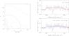 |
Fig. 5 Left: shape of the 68.3%, 90% and 95.4% confidence contours in the (R0, τλ, ∗ ) parameter plane for the two fits to the nitrogen complex. The dotted contours correspond to the assumption that the line in the RGS spectrum is entirely due to N vii λ24.78, whilst the solid contours correspond to the assumption of an equal contribution from the N vi λ24.90 line. The open hexagon and the asterisk correspond to the formal best-fit models. Right: best-fit model (R0 = 3.65 R ∗ , τλ, ∗ = 0.0) assuming a pure N vii line (top) and a blend with N vi λ24.90 (R0 = 3.05 R ∗ , τλ, ∗ = 1.0, bottom panel). Error bars represent ± 1σ (one standard deviation). The feature at –500 km s-1 essentially corresponds to two bins and could be interpreted as the result of noise. Its existence thus needs confirmation. |
Alternatively, we measured the centroid of the observed nitrogen line, defined as
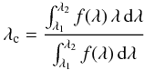 where
λ1 to λ2 are the wavelengths
over which the observed line has a significant level. We find
λc = 24.83 ± 0.01 Å, suggesting that, whilst the nitrogen
complex is dominated by the Lyα line, it is not entirely caused by this
line either.
where
λ1 to λ2 are the wavelengths
over which the observed line has a significant level. We find
λc = 24.83 ± 0.01 Å, suggesting that, whilst the nitrogen
complex is dominated by the Lyα line, it is not entirely caused by this
line either.
Therefore, in what follows, we discuss two situations that we consider as the two
extremes. First, we assume that the nitrogen feature is entirely due to N vii
Lyα. Alternatively, we consider that N vii
Lyα and N vi λ24.90 each account for
half of the emission. We attempted to fit the line with an exospheric line-profile model
following the formalism of Kramer et al. (2003),
although the applicability of such a model to X-ray lines formed in a WR wind has not been
demonstrated yet. The fundamental assumptions of this model are that the X-ray emission
originates in plasma distributed throughout a spherical wind, above a radius
r ≥ R0 > R ∗
and that the hot plasma follows the bulk motion of the cool wind for which we adopted a
β = 1 velocity law. Doppler broadening from macroscopic motion provides
the main source of line broadening. The line emissivity is assumed to scale as
ρ2r − q where
the q term accounts e.g. for a radial dependence of the filling factor of
the X-ray plasma or other phenomena such as a radial variation of shock temperatures,
cooling structures, or change in the relative density of the shocked material (see Kramer
et al. 2003). The free parameters of this model are
thus R0, q (which we choose to be zero as is
often the case for O stars; Güdel & Nazé 2009) and  ,
the characteristic optical depth at wavelength λ. For the terminal
velocity, we adopted v∞ = 2450 km s-1 as derived by
van der Hucht (2001).
,
the characteristic optical depth at wavelength λ. For the terminal
velocity, we adopted v∞ = 2450 km s-1 as derived by
van der Hucht (2001).
Assuming that the nitrogen complex is entirely due to N vii Lyα, the best-fit to the observed line profile is obtained for R0 ~ 3.65 R ∗ and τλ, ∗ = 0. This is illustrated in Fig. 5. The χ2 confidence contours consistently indicate that the model that fits the data must have rather low outward wind optical depth (pointing to a rather low mass-loss rate) and that the X-ray line emission starts at several (~2.5−6.5; 90% confidence limit, Fig. 5) stellar radii. Whilst the derived values are slightly dependent on the assumed value for the terminal velocity, we stress that it remains qualitatively correct that the X-ray emission line is formed above a few stellar radii and that the wind has little optical depth.
On the other hand, if we assume that both N vii Lyα and N vi λ24.90 contribute equal parts to the blend, the best-fit now yields R0 ~ 3.05 R ∗ and τλ,∗ = 1.0. Although the formal best-fit model still indicates a rather low wind optical depth, in this case, the confidence contours include a much wider range of the parameter space.
The relatively low optical depth of the N vii complex is consistent with a moderate mass-loss rate. Such a moderate mass-loss rate is also the interpretation for the triangular profile observed in the visible. However, when looking at the right panels of Fig. 5, one should not forget to consider the error bars that illustrate the uncertainties on this result. The exact morphology of the line needs to be confirmed on the basis of future observations, needed to improve the S/N.
3.3. The X-ray lightcurves
Background-subtracted count rates and totally raw counts (combined pn+MOS1+MOS2) in the various energy bands analysed. Results of the χ2 and of the KS tests.
To study the variability of WR 46 in the X-ray domain, we extracted various lightcurves from the cleaned, but also from the uncleaned, event lists of the three EPIC instruments. The lightcurves were defined in various energy bands. Beyond the usual supersoft, soft, medium, and hard bands, we also selected other intervals basically inspired by the structures as seen in the EPIC spectra (see Fig. 3). These are: 0.2−10.0 keV (the total band), 0.4−0.6 keV (the 0.5 keV bump), 0.55−0.7 keV (the trough in the spectrum), 0.5−2.0 keV (the bulk of the X-ray emission), and finally 2.5−10.0 keV (the high-energy tail). The lightcurves were also binned at various timescales: 200 s, 500 s, 1000 s, and 2000 s. Various statistical tests, as well as a mere eye inspection, were used to scrutinise the different lightcurves. The lightcurves with time bins of 200 and 500 s appear rather noisy. The statistics indeed is very poor (small numbers) and, of course, the situation is getting worse for narrower energy bands. The lightcurves in the 0.55−0.7 keV range are also extremely noisy regardless of the bin size. Also, the EPIC-MOS lightcurves do not contain enough counts to give a lot of information on their own.
As a first step in the analysis, a χ2 test was applied (see e.g. Sana et al. 2004) to all the binned lightcurves. We also applied a Kolmogorov-Smirnov (KS) test, as well as a pov-test (probability of variability test, see again Sana et al. 2004). Finally, we Fourier-analysed all the lightcurves using the generalised technique first described by Heck et al. (1985) and extended by Gosset et al. (2001). We do not report on all the details of the analysis here, but we instead restrict ourselves to the main results. We illustrate our conclusions on the basis of the lightcurves combined from the three-instrument uncleaned event lists, and binned at intervals of 1000 s. The results of the χ2 test on this binned lightcurve are given in Table 4. No time series presents an unlikely high χ2 value. The highest value is associated to the 0.2−0.5 keV energy band. The KS test has been applied to the unbinned lightcurves, and the results are also given in Table 4. It is worth mentioning that, when necessary, we dealt with the presence of bad time intervals (see Sect. 2) by positioning plateaus in the assumed (population) cumulative distribution function at these particular epochs. From the KS test, we conclude that the deviation towards variability is mostly marked in the 0.2−0.5 keV band, but it is not very significant (SL ~ 0.05). The pov-test exhibits no strong deviation, indicating that no flare-like events are present. Some of the lightcurves are illustrated in Fig. 6. Actually the variability is restricted to the supersoft band (it is rather slow), and is not present at all in the 0.5−2.0 keV region. An eye inspection of the figure strongly supports the idea that the variations do not originate in the background.
Consequently, the supersoft band seems to bear most of the variability signal, if any. We could enlarge the band up to 0.6 keV in order to include the main nitrogen line, but this makes no difference in our conclusions. The semi-amplitude spectrum is given in Fig. 7. Clearly a peak is present at ν = 3.032 d-1 (P = 0.3298 d, i.e. 7.9 h), indicating a tendency to reject the white-noise hypothesis in favour of a periodicity or at least of a characteristic timescale. The significance level is estimated to be 0.01. The semi-amplitude related to this frequency is 0.004, which amounts to 15% (30 % full amplitude) of the mean count rate. No other energy band leads to a significant deviation of the semi-amplitude spectrum. The signal is essentially determined by the EPIC-pn detector, which is particularly sensitive in this energy range. The result is also independent of the fact that event lists were cleaned, or not, for bad time intervals. The lightcurve is shown in Fig. 6 where a maximum rate is suspected at both ends of the time series, and an additional one is outstanding in the middle of the interval. This is in good agreement with the frequency found from the Fourier analysis, although we cannot conclude whether there is a pure periodicity since only two cycles are observed. The observed peak-to-peak amplitude near the maximum in the middle of the interval is about 50% of the mean count rate. It is also interesting to notice that the main peak in the semi-amplitude spectrum (Fig. 7) is larger than the expected natural width. Actually the peak extends from 2. to 4. d-1. This could indicate either that the recurrence of the signal is not perfectly periodic or that the signal is not purely monoperiodic. However, when only two cycles are observed, this could also be due to a particular realisation of the noise. We also show in Fig. 6 a similar lightcurve, but one defined in the 0.5−2.0 keV energy range. Clearly the signal is not present. Therefore, we conclude that, during our observations, WR 46 was variable in the very soft part of the spectrum (below about 0.5 keV) with a timescale of 7.9 h but that this signal is not detected in the harder part of the spectrum (above the nitrogen line at 0.5 keV). To the best of our knowledge, this is the first time that such a wavelength-dependent X-ray variability has been observed among WR stars.
It is evidently tempting to relate the single-wave 7.9 h timescale observed in the X-ray with the variability at 6.8−7.8 h detected in the optical domain (including in RVs; see Sect. 1), but it is also striking that the related periodicity in the optical domain corresponds to a double-wave variation in the photometric data.
We partitioned the observed X-ray lightcurve into two parts. One is gathering time intervals related to the period of maximum count rate and the other to minimum count-rate epochs. A spectrum has been extracted corresponding to each part. We found no significant difference either between the two spectra or between the results of the fits we performed on these spectra. The variations in the X-ray flux detected below 0.5 keV are rather small (30% peak-to-peak for a coherent variation and 50% for an occasional one). Such a variation could correspond to a change of the emitted quantity itself or to a change of the absorbing column density δNH of a few 1020 cm-2. The present data are not of sufficient quality to discern between the two possibilities. Any potential reddening corresponding to these amplitude variations being due to a varying column remains undetected in the energy range below 0.5 keV. In addition, a variation due to the column density of 30%, in the energy range 0.2−0.5 keV, implies a variation of less than 10% in the band 0.5−2.0 keV, which could easily remain undetected.
 |
Fig. 6 X-ray lightcurves of WR 46 (background subtracted, binned in 1000 s intervals) in two different energy bands. Upper panel: WR 46 in the 0.2−0.5 keV band; Middle panel: background near the star in the same band; Lower panel: WR 46 in the 0.5−2.0 keV band. The lightcurve corresponds to the combination of the three EPIC instruments (uncleaned event lists). The abscissae give the elapsed time expressed in s; the origin of the time is arbitrary. |
 |
Fig. 7 Semi-amplitude spectrum (i.e. square root of the power spectrum normalized such that the height of the peak corresponds to the semi-amplitude of the relevant cosine curve) of the X-ray lightcurve defined in the 0.2−0.5 keV energy range on the basis of the combination of the three EPIC instruments (uncleaned event lists). The analysed lightcurve was binned into 1000 s intervals; the Nyquist frequency related to the regularity of the lightcurve binning is at ν = 43.2 d-1. |
Unabsorbed X-ray fluxes (0.2−10.0 keV) and luminosities for WR 46.
4. Discussion
4.1. The X-ray luminosity of WR 46
In order to derive the X-ray luminosity of WR 46, we corrected the observed (absorbed) fluxes given in Table 3. We corrected them for an ISM (interstellar medium) column estimated at NH = 0.25 × 1022 cm-2 (see Sect. 3.1). However, if we consider a single column in front of the 3-T mekal, the fitted value amounts to at least NH = 0.54 × 1022 cm-2 (see Table 3); it is roughly twice the one attributed to the ISM. This second value for the column density (labelled “full”) is certainly not to be taken at face value as a possible alternative for the ISM column density, but the fluxes corrected for it may be considered as stringent upper limits. Indeed, the working hypothesis corresponding to the fully corrected fluxes, far more uncertain, relies on the assumptions that all the plasma components have a common location behind the full column and that the effect of the fitted neutral column is actually representative of the true physical absorption, which might not be the case. The unabsorbed X-ray fluxes (0.2−10.0 keV energy range) are given in Table 5. They have thus been corrected for the ISM absorbing column and, to fix ideas, for the full column density. The models used correspond to those given in Table 3. We give, for the same energy band, the luminosities (corrected either for the NH = 0.25 × 1022 cm-2 ISM column or for the full column and supposing the object is at 4 kpc). Every first line deals with the fit to the EPIC data, whereas every second line deals with the simultaneous EPIC+RGS fit.
The fluxes computed on the basis of the different models that we used (see Tables 2 and 3) are
very similar which gives further weight to the derived values. If we adopt an observed
flux  = 1.3 ×
10-13 erg cm-2 s-1, and if we correct it for the ISM
column density, we deduce an intrinsic flux
= 1.3 ×
10-13 erg cm-2 s-1, and if we correct it for the ISM
column density, we deduce an intrinsic flux  = 4.0 ×
10-13 erg cm-2 s-1 and a luminosity for a distance of
d kpc of LX(0.2−10.0 keV) = 4.8 ×
1031 d2 kpc-2 erg s-1. If
we perform the same computation for other energy bands, we arrive at similar luminosities
of LX(0.2−4.0 keV) = 4.6 ×
1031 d2 kpc-2 erg s-1 and
LX(0.2−2.4 keV) = 4.3 ×
1031 d2 kpc-2 erg s-1. This
first WR 46 luminosity is in good agreement with the value
3.5 × 1033 erg s-1 reported by Pollock (1987) on the basis of EINSTEIN observations of WR 46
and of an assumed distance of 8.7 kpc. The second one is also in reasonably good agreement
with the value LX(0.2−2.4 keV) = 2.5 ×
1032 erg s-1 reported from ROSAT data
(Wessolowski 1996, with a derived distance of
2.5 kpc). This suggests some long-term stability of the X-ray luminosity of WR 46.
= 4.0 ×
10-13 erg cm-2 s-1 and a luminosity for a distance of
d kpc of LX(0.2−10.0 keV) = 4.8 ×
1031 d2 kpc-2 erg s-1. If
we perform the same computation for other energy bands, we arrive at similar luminosities
of LX(0.2−4.0 keV) = 4.6 ×
1031 d2 kpc-2 erg s-1 and
LX(0.2−2.4 keV) = 4.3 ×
1031 d2 kpc-2 erg s-1. This
first WR 46 luminosity is in good agreement with the value
3.5 × 1033 erg s-1 reported by Pollock (1987) on the basis of EINSTEIN observations of WR 46
and of an assumed distance of 8.7 kpc. The second one is also in reasonably good agreement
with the value LX(0.2−2.4 keV) = 2.5 ×
1032 erg s-1 reported from ROSAT data
(Wessolowski 1996, with a derived distance of
2.5 kpc). This suggests some long-term stability of the X-ray luminosity of WR 46.
4.2. The nature of WR 46: Wolf-Rayet versus SSS
As mentioned earlier in this paper, WR46 has sometimes been associated to the SSS class of objects. It is therefore relevant to addressing the question of the nature of WR46 (i.e. WR vs SSS) in the light of the information obtained through our X-ray data. Most SSS objects seem to present an X-ray spectrum which can be interpreted as the emission of a high-gravity hot photosphere of a white dwarf and is thus the X-ray transposition of a typical visible spectrum with large absorption troughs superimposed onto a continuum (see Paerels et al. 2001; Reinsch et al. 2006). However, Orio et al. (2004) report an X-ray emission-line spectrum for CAL 87, a well-known SSS presenting redshifted lines with a velocity in the range of 700−1200 km s-1. In such a case, the wind could be that of an accretion disk in a close binary system including a white dwarf. It should, however, be pointed out that the X-ray spectrum of CAL 87 is not typical of all SSSs. WR 46, with its emission lines, would be more reminiscent of CAL 87.
The level of luminosity derived in the previous section is quite representative of what is usually found for WR stars (see e.g. Wessolowski 1996). This is clearly less than the 1036 to 1038 erg s-1 (or larger) measured for the SSSs (see Greiner 2000). The luminosity is, of course, dependent on the assumed distance. A much less dependent value is the log LX/Lbol ratio that is computed to be about –6.2 to –6.5. Such a ratio is also more reminiscent of an early-type star rather than of an SSS (Greiner 2000). However, the value depends on the applied bolometric correction, which is quite important (–5.9) for WR 46 if it is considered as a true WR star. The value of the log LX/Lbol ratio thus depends on the assumption on the nature of the star. To further ascertain our conclusion, we also computed the log LX/LV ratio. For WR 46, we computed log LX/LV = −3.0. The importance of the luminosity in visible light also favours the WR nature since most of the emission of an SSS is in the X-ray domain. The XMM-Newton spectrum of WR46 presents a significant medium-hard X-ray emission tail and an Fe-K line that are not expected in the spectrum of SSSs, even for peculiar cases such as CAL 87. The latter are indeed characterised by a very soft X-ray spectrum (typically with temperatures below 100 eV, never emitting above 1 keV), as quoted for instance by Greiner (2000). The SSS identification is thus clearly ruled out.
The probable enrichment in nitrogen observed in the X-ray spectrum emitted by WR46 is reminiscent of WR stars, although the observed enhancement is only approximately measured and could be much less than those typical of WR stars. The apparent absence of hydrogen in WR 46 (Crowther et al. 1995) also favours its WR nature, though it should be noted that the position of WR 46 is also slightly out of the WR locus in the luminosity-temperature diagram (on the hot side, see Hamann et al. 2006). It is thus also slightly anomalous for a WR star.
4.3. The origin of the X-ray emission
A range of temperatures is necessary to interpret the observed EPIC spectra. We successfully modelled the data with absorbed emission from multi-temperature, optically thin, thermal plasma models and repertoried the three following temperatures: 0.1−0.2 keV, 0.6 keV, and ~4.0 keV. Although the three numbers are certainly not to be taken at face value, they are indicative of the variety of temperatures present in the global emitting volume.
4.3.1. The soft spectrum
A plasma temperature of 0.6−0.8 keV is usually dominant in massive OB stars (see e.g. Sana et al. 2006; Nazé 2009). This X-ray emission is generally attributed to a warm plasma that is heated by strong hydrodynamical shocks intrinsic to the stellar wind (see Sect. 1). In this context, the plasma temperature of 0.6 keV derived from the spectral modelling translates into a post-shock temperature of the order of 7 × 10⁶ K, corresponding to a pre-shock velocity of about 600 km s-1. Such a pre-shock velocity is typical of hydrodynamical shocks expected to occur within the unstable stellar wind (e.g. Feldmeier et al. 1997). The presence of a plasma at a temperature in the range 0.3−0.6 keV is also a characteristic of several X-ray emitting WN stars (see e.g. Skinner et al. 2010), whatever their nature.
The exact shape of the Lyα line of N vii at 0.5 keV (24.78 Å) is very important in this context. Our results of Sect. 3.2 seem to suggest that the N vii λ24.78 nitrogen line is rather wide (3500 km s-1) and is almost flat-topped or only slightly asymmetric implying the existence of very little opacity in the line. The impossibility of choosing between these two latter cases originates in the impact of the soft plasma temperature and of the relative strength of the N vi λ24.90 line. In either case, the large width of the observed line and its rather flat-topped shape are suggested by the present data but certainly deserve confirmation. Such a flat-topped shape, or nearly so, is reminiscent of what is expected to arise from a spherical symmetric emission shell (Kramer et al. 2003), and this suggests that the X-ray emission could originate in the shocked wind of the WN star. This line shape is very crucial because it is different from the profile that should be produced in the context of a magnetically channelled wind (Gagné et al. 2005). This is also true for the large width. The flat-topped line shape is also different from the profiles predicted in the framework of a colliding-wind binary (Henley et al. 2005, 2008). If the last two mechanisms contribute to some extent to the Lyα line of N vii, the fit suggests that it is through a minor contribution. The N overabundance associated with the soft plasma is another argument that links (predominantly) this emitting plasma with the wind of the WN component.
4.3.2. The hard spectrum
In the context of the X-ray emission from massive stars, several scenarios can be envisaged to explain a hard emission component. As the spectral modelling described in Sect. 3.1 suggests a thermal X-ray emission, we restrict the discussion to thermal emission processes or to scenarios likely to mimic a thermal emission, such as the production of an iron K line on top of a nonthermal continuum (a low signal-to-noise hard spectrum may not allow distinguishing these two cases). We neglect purely nonthermal processes, such as those described by De Becker (2007).
The intrinsic X-ray emission discussed in the previous section is not able to explain a component at ~4 keV and the presence of its associated iron K line. To heat a plasma up to temperatures of 4 keV, the pre-shock velocity of the plasma should reach a typical value of at least 1650 km s-1, which is much too high for intrinsic shocks (at most several 100 km s-1). However, such pre-shock velocities are reached in the context of colliding-wind binaries whose period is longer than a few weeks. This condition on the period should be fulfilled in order to allow the stellar winds to reach a high fraction of their terminal velocities before colliding. Several WR (essentially WN) stars are known to exhibit a two-component plasma at 0.6 keV and 3−4 keV (some O stars too), in a similar way as WR 46. Some of them, like WR 22 (Rauw et al. 1996; Gosset et al. 2009) or WR 25 (Raassen et al. 2003; Gamen et al. 2006) are known to be long-period binaries, but others are still considered as single because of not having any firm detection of a companion (WR 6, Skinner et al. 2002b; WR 110, Skinner et al. 2002a). Skinner et al. (2010) doubt that all of them could be binaries and argue that we should be ready to recognise that this hard component could be intrinsic to single WN stars and could thus be attributed to a yet unidentified mechanism. In addition to the hard tail, the value of LX/Lbol quoted in Sect. 4.2 indicates a small excess with respect to the law for single massive O stars, which could be the sign of a colliding-wind phenomenon. The applicability of the colliding wind interpretation to WR 46 is not clear, since there is so far no other hint of a companion orbiting with a period that is long enough. Nevertheless, this scenario should not be neglected.
Beside the interaction between stellar winds in a massive binary, the accretion of wind material onto a degenerate star (black hole or neutron star) is likely to produce a significant amount of hard X-rays. In such a case, we would be dealing with an object belonging to the class of High Mass X-ray Binaries (HMXB) or even microquasars. X-ray spectra of such objects can be well reproduced by a black body emission component, or by a power law with an additional fluorescence iron K line produced by the bombardment by high energy photons from the accretion disk. However, such objects are expected to be very bright high-energy sources, with typical X-ray luminosities in the EPIC bandpass higher than 1033 erg s-1, up to 1035–1036 erg s-1 for the brightest ones (e.g. Sidoli et al. 2006; Bosch-Ramon et al. 2007; Tomsick et al. 2009). Such X-ray luminosities are significantly higher than what we determined, and the occurrence of any HMXB-like processes in WR 46 is unlikely. In addition, the long-term stability of the X-ray luminosity of WR 46 does not support the scenario of accretion onto a compact object.
Finally, in the context of single stars, magnetically confined-wind-shock models such as described by Babel & Montmerle (1997) and ud-Doula & Owocki (2002), are expected to be able to heat plasmas up to temperatures of several tens of MK, sufficient to generate a hard X-ray spectrum (e.g. Schulz et al. 2003). The winds from both hemispheres undergo a head-on collision near the magnetic equator, and this produces a plasma hotter than in a classical wind embedded shock situation. A contribution to the EPIC spectrum of WR 46 arising from such a process may therefore constitute a plausible scenario for interpreting the hard tail. We caution, however, that such models consider an efficient magnetic confinement in the inner part of the wind where the N vii Ly α line is expected to be produced, and we showed above that its apparent spectral profile is not compatible with such models that rather predict narrow lines. Moreover, this approach would be much more relevant if some evidence of a strong magnetic field were available, but this argument is weakened by the fact that a magnetic field would be extremely difficult to proove in such an object. We do not consider this scenario to be adequate.
In summary, we consider that the most plausible explanation for the hard X-ray tail observed in the EPIC spectrum is the presence of a companion orbiting on a period longer than a few weeks, whose stellar wind interacts with that of the WN star. We note that the several hundreds of days timescale reported by Marchenko et al. (1998) on the basis of Hipparcos photometry may provide some support to this scenario. Plausible alternatives are not yet identified, though other massive objects present a similar tail.
4.4. The soft X-ray variability
As discussed above, the criterion on the period of a potential binary disqualifies definitely the 7.9 h timescale discovered in the soft part of the spectrum as the orbital period of a potential companion whose wind-wind interaction produces the hard tail. We therefore consider that the mechanisms responsible for this short-term variability and for the production of the hard tail could be completely independent.
Let us first investigate the scenario where the 7.9 h timescale is the period of a very close binary. Such a short period implies a rather tight system. If we adopt either K = 50 km s-1 or K = 75 km s-1 as the semi-amplitude of the radial velocity curve of the WN component, the total separation asini of the system is expected to be around 0.7 R⊙ to 10 R⊙, depending on the relative mass of the companion. The two values are given respectively for MWN = Mcomp and MWN = 20 Mcomp. The range of line-of-sight projected separations above 1−2 R⊙ corresponds to low-mass stars that are certainly not able to develop a wind to effectively interact with the WN one. There is thus no room to include a companion producing a wind in a possible P = 0.3 d orbiting system except for inclinations lower than about 10°. In this particular case, one would expect little photometric variability associated to this periodicity. In addition, if a companion was so close, it would be surprising that its presence does not perturb the profile of the N vii line.
Even though a very close binary of the kind WN + OB is unlikely to produce a wind-wind interaction responsible for the hard tail, it is worth considering a scenario where the wind of the WN star crushes onto the surface of a much lower mass companion star orbiting in a very close orbit. Such a system could lead to a low-emission-measure X-ray emitting region associated to the shocked plasma on the surface of the secondary star. The X-ray contribution from such a system would be very sensitive to orientation effects, depending on geometrical considerations and on the orbital phase, and could lead to low-amplitude variations, particularly in the soft band. However, such a scenario is much too speculative to lead to quantitative discussions aiming at explaining the observed variations. On the other hand, if the putative close, low-mass companion is a degenerate object, the accretion of the inner wind material onto its surface would be expected to produce a large quantity of X-rays in a way reminiscent of what is observed for HMXBs. As underlined in Sect. 4.3.2, such sources are expected to produce a very bright variable black body or power-law X-ray spectrum, which completely contradicts the moderately bright emission line EPIC spectrum of WR 46.
Finally, in the absence of a close companion, the origin of the low-amplitude variability detected in soft X-rays may be intrinsic to the wind of the WN star. This is further supported by the fact that the nitrogen lines seem to be associated with the WN wind. The structure of stellar winds of massive stars is still a matter of debate, but it is commonly admitted that massive star winds are not always spherical and homogeneous. Besides the small-scale structures related to instabilities in the line-driving mechanism, large-scale density structures with dimensions typical of the stellar radius are expected to be present as well. Among such structures, one may consider corotating structures confined by the stellar magnetic field. The magnetic field must in this case be weaker than the one confining the whole wind as discussed in Sect. 4.3.2. Explaining variability in X-rays should generally consider two effects, the emission process, and the absorption. As both thermal emission and absorption processes intimately depend on the density, both can be significantly affected by any large-scale structure corotating with the star. This case corresponds to the Large-Scale Corotating Structures (LSCS) scenario discussed by De Becker et al. (2009) to explain the line profile variability in the visible spectrum exhibited by a few O-type supergiants on the way to the WN type. The density structures might affect the intrinsic shocks in the wind and directly induce the observed variations. The latter will be modulated by the rotation cycle of the star. This necessitates fine tuning the model to avoid the hard X-ray emission typical of confined winds and to avoid any detectable change of the N vii Lyα profile (although the S/N is very low).
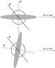 |
Fig. 8 Schematic view of an oblique rotator presenting a large-scale corotating structure (in grey) in the inner part of the wind of the WN star. θ and φ stand for the rotation and magnetic axes, respectively. In the upper configuration, the line of sight crosses the large-scale structure, therefore maximizing the absorption of the soft X-rays emitted at the base of the stellar wind. The lower configuration illustrates the relative position of the large-scale structure with respect to the line of sight half a rotational period later. In that case, we may expect a maximum in the soft X-ray lightcurve. |
An interesting alternative explanation consists in invoking the existence in the wind of Corotating Interaction Regions (CIRs, see e.g. Cranmer & Owocki 1996; but also Dessart & Chesneau 2002; St-Louis et al. 2009). Such a phenomenon generated by altered physical conditions at the basis (critical point) of the wind perturbs velocities and creates density fluctuations propagating outwards and spiralling with respect to the rotation axis. The rotation clock of the star is thus enshrined in the CIR structure. The initial perturbation could come from a magnetic field (even weak) close to the surface. The CIR structure could persist up to a few tens of stellar radii (Dessart & Chesneau 2002) and could thus present density fluctuations well above the formation region of the soft X-ray lines. The density variations could induce the observed variations. A CIR structure could also develop from pulsations and in particular from the beats of modes (see e.g. Gosset & Rauw 2009). The mechanism of X-ray emission in intrinsically shocked winds is not understood well enough to lead to firm conclusions, but it is very likely that pulsations could create the observed 30−50% fluctuations in flux. On the other hand, regardless of their origin, the CIR could also exhibit density fluctuations (able to attenuate the whole line-forming region) of 10−20% (δNH a few 1020 cm-2), which are enough to explain the observed X-ray luminosity variations. This interpretation is the most likely one.
5. Conclusions
On the basis of X-ray observations of the enigmatic object WR 46 (spectral type WN3pec), we definitely conclude that this object does not at all resemble the SSSs. The X-ray luminosity of the object is of the order of LX(0.2−10.0 keV) = 4.8 × 1031 d2 kpc-2 erg s-1 which is much lower than what is usually observed for the SSS objects (1038–1039 erg s-1). In addition, WR 46 exhibits a harder tail that does not exist for these objects. Actually, WR 46 has a luminosity that is more related to those usually associated to WR stars provided its presumed distance is not wrong by a large amount. The LX/Lbol ratio computed for WR 46 indicates a value larger by 0.5 dex if compared to the OB star scaling law (10-7 ratio). If this OB ratio applied to WR stars, this could indicate a slight excess of X-ray emission.
The X-ray spectrum of WR 46 is rather well fitted by a three-temperature, optically thin, thermal plasma model (at equilibrium): 0.1−0.2 keV, 0.6 keV, and ~4 keV. They physically represent a range of temperature clearly present in the hot plasma around the star. Although little is known about the intrinsic emission of WN stars, the single OB stars usually exhibit plasmas at a dominant temperature of 0.6−0.8 keV, often accompanied by a cooler 0.2 keV component (see Sana et al. 2006; Nazé 2009) that are generally attributed to shocked winds generated by the genuine instabilities typical of radiatively driven outflows. The soft part of the WR spectrum covered by the two lower temperatures has been observed at high resolution (with the RGS), and only one exploitable line clearly dominates the RGS spectrum: N vii λ24.78. This line appears broad with a large half width of 1750 km s-1. If the plasma temperature could be as low as 0.1 keV or below, the line could be blended with another nitrogen line, but this does not change our conclusions much. The nitrogen line is well fitted by an exospheric model and, if confirmed, instead supports the shocked wind hypothesis. The nitrogen overabundance of the fitted plasma suggests a relation between the emitting plasma and the wind of the WN3 object. The width of the line also points to this direction.
The third temperature, indicating a hard tail, is usually considered too high to be explained by shocks in the wind of a single star. The presence of the Fe-K line often but not always indicates a stronger shock. This stronger shock is more reminiscent of a wind-wind collision zone associated with an object orbiting on a period of at least a few weeks. This condition on the period arises from the requirement to allow the stellar winds to collide with an adequate pre-shock velocity. A very close companion (in a P = 7.9 h orbital system) will not be massive enough to develop a wind able to compete with the WR one. However, a distant companion has not been detected so far, and a 3−4 keV component is rather common in WN stars, including some presumably single stars (see e.g. WR 6, Skinner et al. 2002b; 2010).
We also detect a significant – although weak – variation in the soft X-ray flux (between 0.2 and 0.5 keV) with a timescale of roughly 7.9 h, compatible with the 7−9 h period or pseudo-period associated to optical line radial velocities and visible photometry. The X-ray observations are, however, single-wave. To the best of our knowledge, this is the first time that such a variability is reported for a WR star. Our data preclude to discern between an intrinsic luminosity variation and a change in the local extinction. Above 0.5 keV, the flux exhibits no clear variations. Even though the origin of this variability is not clearly identified, corotating large-scale density structures or, better, CIRs originating in the inner wind of the WN star are worth considering. The deep cause could be a magnetic field, but a more viable alternative is the presence of CIRs induced by pulsations.
WR 46 is a very interesting object and certainly more about it will be known when we will be able to confirm the profile of the X-ray lines related to the soft plasma and to access the X-ray line profiles related to the hard one.
Acknowledgments
We warmly thank Hugues Sana for help in reducing the FEROS spectrum of Fig. 1. We are grateful to the Belgian FNRS for multiple support. We also acknowledge financial support through the XMM-OM and the XMM and the INTEGRAL PRODEX contracts, as well as through the PAI contract P5/36 (Belspo). Finally a recent contract by the Communauté Française de Belgique (Action de Recherche Concertée) – Académie Wallonie-Europe is also acknowledged.
References
- Anders, E., & Grevesse, N. 1989, Geochem. Cosmochim. Acta, 53, 197 [Google Scholar]
- Arnaud, K. A. 1996, in Astronomical Data Analysis Software and Systems V, ed. G. H. Jacoby, & J. Barnes, PASP Conf. Ser., 101, 17 [Google Scholar]
- Arnaud, K. A. 1999, BAAS, 31, 734 [NASA ADS] [Google Scholar]
- Babel, J., & Montmerle, T. 1997, ApJ, 485, L29 [NASA ADS] [CrossRef] [Google Scholar]
- Berghöfer, T. W., Schmitt, J. H. M. M., Danner, R., & Cassinelli, J. P. 1997, A&A, 322, 167 [NASA ADS] [Google Scholar]
- Bosch-Ramon, V., Motch, C., Ribó, M., et al. 2007, A&A, 473, 545 [NASA ADS] [CrossRef] [EDP Sciences] [Google Scholar]
- Cannon, A. J. 1916, Harvard College Observatory Annals, 76, 19 [Google Scholar]
- Cassinelli, J. P., Waldron, W. L., Sanders, W. T., et al. 1981, ApJ, 250, 677 [NASA ADS] [CrossRef] [Google Scholar]
- Chlebowski, T., Harnden, F. R. Jr., & Sciortino, S. 1989, ApJ, 341, 427 [NASA ADS] [CrossRef] [Google Scholar]
- Conti, P. S., & Vacca, W. D. 1990, AJ, 100, 431 [Google Scholar]
- Corcoran, M. F., Waldron, W. L., McFarlane, J. J., et al. 1994, ApJ, 436, L95 [NASA ADS] [CrossRef] [Google Scholar]
- Cowley, A. P., Schmidtke, P. C., Hutchings, J. B., Crampton, D., & McGrath, T. K. 1993, ApJ, 418, L63 [NASA ADS] [CrossRef] [Google Scholar]
- Cranmer, S. R., & Owocki, S. P. 1996, ApJ, 462, 469 [NASA ADS] [CrossRef] [Google Scholar]
- Crowther, P. A., Smith, L. J., & Hillier, D. J. 1995, A&A, 302, 457 [NASA ADS] [Google Scholar]
- De Becker, M. 2007, A&ARv, 14, 171 [NASA ADS] [CrossRef] [Google Scholar]
- De Becker, M., Rauw, G., & Linder, N. 2009, ApJ, 704, 964 [NASA ADS] [CrossRef] [Google Scholar]
- den Herder, J. W., Brinkman, A. C., Kahn, S. M., et al. 2001, A&A, 365, L7 [NASA ADS] [CrossRef] [EDP Sciences] [Google Scholar]
- Dessart, L., & Chesneau, O. 2002, A&A, 395, 209 [NASA ADS] [CrossRef] [EDP Sciences] [Google Scholar]
- Dietrich, J. P., Miralles, J. M., Olsen, L. F., et al. 2006, A&A, 449, 837 [NASA ADS] [CrossRef] [EDP Sciences] [Google Scholar]
- Feldmeier, A., Puls, J., & Pauldrach, A. W. A. 1997, A&A, 322, 878 [NASA ADS] [Google Scholar]
- Fleming, W. P. 1910, Harvard College Observatory Circ., 158, 1 [NASA ADS] [Google Scholar]
- Fleming, W. P. 1912, Harvard College Observatory Annals, 56, 165 [Google Scholar]
- Gagné, M., Oksala, M. E., Cohen, D. H., et al. 2005, ApJ, 628, 986; Erratum: 634, 712 [NASA ADS] [CrossRef] [Google Scholar]
- Gamen, R., Gosset, E., Morrell, N., et al. 2006, A&A, 460, 777 [NASA ADS] [CrossRef] [EDP Sciences] [Google Scholar]
- Gosset, E. 2007, Études d’étoiles massives de types spectraux O, Wolf-Rayet et apparentés. Résultats de campagnes d’observations photométriques et spectroscopiques dans le domaine visible et dans le domaine des rayons X, Agrégation de l’Enseignement Supérieur, Université de Liège [Google Scholar]
- Gosset, E., & Rauw, G. 2009, in Evolution and Pulsation of Massive Stars on the Main Sequence and Close to it, 38th Liège Int. Ast. Coll., ed. A. Noels et al., CoAst, 158, 138 [Google Scholar]
- Gosset, E., Royer, P., Rauw, G., Manfroid, J., & Vreux, J.-M. 2001, MNRAS, 327, 435 [NASA ADS] [CrossRef] [Google Scholar]
- Gosset, E., Nazé, Y., Claeskens, J.-F., et al. 2005, A&A, 429, 685 [NASA ADS] [CrossRef] [EDP Sciences] [Google Scholar]
- Gosset, E., Nazé, Y., Sana, H., Rauw, G., & Vreux, J.-M. 2009, A&A, 508, 805 [NASA ADS] [CrossRef] [EDP Sciences] [Google Scholar]
- Greiner, J. 2000, New Astron., 5, 137 [NASA ADS] [CrossRef] [Google Scholar]
- Güdel, M., & Nazé, Y. 2009, A&ARv, 17, 309 [NASA ADS] [CrossRef] [Google Scholar]
- Hamann, W. R., Gräfener, G., & Liermann, A. 2006, A&A, 457, 1015 [NASA ADS] [CrossRef] [EDP Sciences] [Google Scholar]
- Heck, A., Manfroid, J., & Mersch, G. 1985, A&AS, 59, 63 [Google Scholar]
- Henley, D. B., Stevens, I. R., & Pittard, J. M. 2005, MNRAS, 356, 1308 [NASA ADS] [CrossRef] [Google Scholar]
- Henley, D. B., Corcoran, M. F., Pittard, J. M., et al. 2008, ApJ, 680, 705 [NASA ADS] [CrossRef] [Google Scholar]
- Ignace, R., & Oskinova, L. 1999, A&A, 348, L45 [NASA ADS] [Google Scholar]
- Jansen, F., Lumb, D., Altieri, B., et al. 2001, A&A, 365, L1 [NASA ADS] [CrossRef] [EDP Sciences] [Google Scholar]
- Kaastra, J. S. 1992, An X-ray spectral code for optically thin plasmas, Internal SRON-Leiden Report [Google Scholar]
- Koyama, K., Maeda, Y., Tsuru, T., Nagase, F., & Skinner, S. 1994, PASJ, 46, L93 [NASA ADS] [Google Scholar]
- Kramer, R. H., Cohen, D. H., & Owocki, S. P. 2003, ApJ, 592, 532 [NASA ADS] [CrossRef] [Google Scholar]
- Lemen, J. R., Mewe, R., Schrijver, C. J., & Fludra, A. 1989, ApJ, 341, 474 [NASA ADS] [CrossRef] [Google Scholar]
- Long, K. S., & White, R. L. 1980, ApJ, 239, L65 [NASA ADS] [CrossRef] [Google Scholar]
- Lucy, L. B. 1982, ApJ, 255, 286 [NASA ADS] [CrossRef] [Google Scholar]
- Lucy, L. B., & White, R. L. 1980, ApJ, 241, 300 [NASA ADS] [CrossRef] [Google Scholar]
- Lynga, G., & Wramdemark, S. 1973, A&AS, 12, 365 [Google Scholar]
- Maeda, Y., Koyama, K., Yokogawa, J., & Skinner, S. 1999, ApJ, 510, 967 [NASA ADS] [CrossRef] [Google Scholar]
- Marchenko, S. V., Moffat, A. F. J., van der Hucht, K. A., et al. 1998, A&A, 331, 1022 [NASA ADS] [Google Scholar]
- Marchenko, S. V., Arias, J., Barbá, R., et al. 2000, AJ, 120, 2101 [NASA ADS] [CrossRef] [Google Scholar]
- Marchenko, S. V., Moffat, A. F. J., Crowther, P. A., et al. 2004, MNRAS, 353, 153 [NASA ADS] [CrossRef] [Google Scholar]
- Mewe, R., Gronenschild, E. H. B. M., & van den Oord, G. H. J. 1985, A&AS, 62, 197 [Google Scholar]
- Monderen, P., De Loore, C. W. H., van der Hucht, K. A., & van Genderen, A. M. 1988, A&A, 195, 179 [NASA ADS] [Google Scholar]
- Morris, P. W., Brownsberger, K. R., Conti, P. S., Massey, P., & Vacca, W. D. 1993, ApJ, 412, 324 [NASA ADS] [CrossRef] [Google Scholar]
- Nazé, Y. 2009, A&A, 506, 1055 [NASA ADS] [CrossRef] [EDP Sciences] [Google Scholar]
- Niemela, V. S., Barbá, R. H., & Shara, M. M. 1995, in Wolf-Rayet Stars: Binaries, Colliding Winds, Evolution, ed. K. A. van der Hucht, & P. M. Williams, (Dordrecht: Kluwer Acad. Publ.), IAU Symp., 163, 245 [Google Scholar]
- Oliveira, A. S., Steiner, J. E., & Diaz, M. P. 2004, PASP, 116, 311 [NASA ADS] [CrossRef] [Google Scholar]
- Orio, M., Ebisawa, K., Heise, J., & Hartmann, W. 2004, Rev. Mex. Astron. Astrofis. Ser. Conf., 20, 210 [NASA ADS] [Google Scholar]
- Oskinova, L. M., Ignace, R., Hamann, W. R., Pollock, A. M. T., & Brown, J. C. 2003, A&A, 402, 755 [NASA ADS] [CrossRef] [EDP Sciences] [Google Scholar]
- Paerels, F., Rasmussen, A. P., Hartmann, H. W., et al. 2001, A&A, 365, L308 [NASA ADS] [CrossRef] [EDP Sciences] [Google Scholar]
- Pallavicini, R., Golub, L., Rosner, R., et al. 1981, ApJ, 248, 279 [NASA ADS] [CrossRef] [Google Scholar]
- Parthasarathy, M., Branch, D., Jeffery, D. J., & Baron, E. 2007, New Astron. Rev., 51, 524 [NASA ADS] [CrossRef] [Google Scholar]
- Perryman, M. A. C., Lindegren, L., Kovalevsky, J., et al. 1997, A&A, 323, L49 [NASA ADS] [Google Scholar]
- Pittard, J. M., Stevens, I. R., Williams, P. M., et al. 2002, A&A, 388, 335 [NASA ADS] [CrossRef] [EDP Sciences] [Google Scholar]
- Pollock, A. M. T. 1987, ApJ, 320, 283 [NASA ADS] [CrossRef] [Google Scholar]
- Pollock, A. M. T., & Corcoran, M. F. 2006, A&A, 445, 1093 [NASA ADS] [CrossRef] [EDP Sciences] [Google Scholar]
- Pollock, A. M. T., Haberl, F., & Corcoran, M. F. 1995, in Wolf-Rayet Stars: Binaries, Colliding Winds, Evolution, ed. K. A. van der Hucht, & P. M. Williams, (Dordrecht: Kluwer Acad. Publ.), IAU Symp., 163, 512 [Google Scholar]
- Pollock, A. M. T., Corcoran, M. F., Stevens, I. R., & Williams, P. M. 2005, ApJ, 629, 482 [NASA ADS] [CrossRef] [Google Scholar]
- Raassen, A. J. J., van der Hucht, K. A., Mewe, R., et al. 2003, A&A, 402, 653 [NASA ADS] [CrossRef] [EDP Sciences] [Google Scholar]
- Rauw, G., Vreux, J.-M., Gosset, E., et al. 1996, A&A, 306, 771 [NASA ADS] [Google Scholar]
- Reinsch, K., Burwitz, V., & Schwarz, R. 2006, in The X-ray Universe 2005, ed. A. Wilson, ESA SP-604, 285 [Google Scholar]
- Sana, H., Stevens, I. R., Gosset, E., Rauw, G., & Vreux, J.-M. 2004, MNRAS, 350, 809 [NASA ADS] [CrossRef] [Google Scholar]
- Sana, H., Rauw, G., Nazé, Y., Gosset, E., & Vreux, J.-M. 2006, MNRAS, 372, 661 [NASA ADS] [CrossRef] [Google Scholar]
- Schild, H., Güdel, M., Mewe, R., et al. 2004, A&A, 422, 177 [NASA ADS] [CrossRef] [EDP Sciences] [Google Scholar]
- Schulz, N. S., Canizares, C., Huenemoerder, D., & Tibbets, K. 2003, ApJ, 595, 365 [NASA ADS] [CrossRef] [Google Scholar]
- Sciortino, S., Vaiana, G. S., Harnden, F. R. Jr., et al. 1990, ApJ, 361, 621 [NASA ADS] [CrossRef] [Google Scholar]
- Seward, F. D., & Chlebowski, T. 1982, ApJ, 256, 530 [NASA ADS] [CrossRef] [Google Scholar]
- Sidoli, L., Pellizzoni, A., Vercellone, S., et al. 2006, A&A, 459, 901 [NASA ADS] [CrossRef] [EDP Sciences] [Google Scholar]
- Singh, K. P., White, N. E., & Drake, S. A. 1996, ApJ, 456, 766 [NASA ADS] [CrossRef] [Google Scholar]
- Skinner, S. L., Zhekov, S. A., Güdel, M., & Schmutz, W. 2002a, ApJ, 572, 477 [NASA ADS] [CrossRef] [Google Scholar]
- Skinner, S. L., Zhekov, S. A., Güdel, M., & Schmutz, W. 2002b, ApJ, 579, 764 [NASA ADS] [CrossRef] [Google Scholar]
- Skinner, S. L., Güdel, M., Schmutz, W., & Zhekov, S. 2006, Ap&SS, 304, 97 [NASA ADS] [CrossRef] [Google Scholar]
- Skinner, S. L., Zhekov, S. A., Güdel, M., Schmutz, W., & Sokal, K. R. 2010, AJ, 139, 825 [NASA ADS] [CrossRef] [Google Scholar]
- Smith, H. J. 1955, Thesis Harvard College Observatory, 130 (see AJ, 60, 180) [Google Scholar]
- Smith, L. F. 1968, MNRAS, 140, 409 [NASA ADS] [Google Scholar]
- Smith, L. F., Shara, M. M., & Moffat, A. F. J. 1996, MNRAS, 281, 163 [NASA ADS] [CrossRef] [Google Scholar]
- Smith, M. A., Cohen, D. H., Gu, M. F., et al. 2004, ApJ, 600, 972 [NASA ADS] [CrossRef] [Google Scholar]
- St-Louis, N., Chené, A. N., Schnurr, O., & Nicol, M. H. 2009, ApJ, 698, 1951 [NASA ADS] [CrossRef] [Google Scholar]
- Steiner, J. E., & Diaz, M. P. 1998, PASP, 110, 276 [NASA ADS] [CrossRef] [Google Scholar]
- Stevens, I. R., Blondin, J. M., & Pollock, A. M. T. 1992, ApJ, 386, 265 [NASA ADS] [CrossRef] [Google Scholar]
- Stevens, I. R., Corcoran, M. F., Willis, A. J., et al. 1996, MNRAS, 283, 589 [NASA ADS] [Google Scholar]
- Strüder, L., Briel, U., Dennerl, K., et al. 2001, A&A, 365, L18 [NASA ADS] [CrossRef] [EDP Sciences] [Google Scholar]
- Tomsick, J. A., Chaty, S., Rodriguez, J., et al. 2009, ApJ, 694, 344 [NASA ADS] [CrossRef] [Google Scholar]
- Tovmassian, H. M., Navarro, S. G., & Cardona, O. 1996, AJ, 111, 306 [NASA ADS] [CrossRef] [Google Scholar]
- Turner, M. J. L., Abbey, A., Arnaud, M., et al. 2001, A&A, 365, L27 [NASA ADS] [CrossRef] [EDP Sciences] [Google Scholar]
- ud-Doula, A., & Owocki, S. P. 2002, ApJ, 576, 413 [NASA ADS] [CrossRef] [Google Scholar]
- van der Hucht, K. A. 2001, New Astron. Rev., 45, 135 [NASA ADS] [CrossRef] [Google Scholar]
- van der Hucht, K. A., Cassinelli, J. P., & Williams, P. M. 1986, A&A, 168, 111 [NASA ADS] [Google Scholar]
- van der Hucht, K. A., Hidayat, B., Admiranto, A. G., Supelli, K. R., & Doom, C. 1988, A&A, 199, 217 [NASA ADS] [Google Scholar]
- van Genderen, A. M., van der Hucht, K. A., & Larsen, I. 1990, A&A, 229, 123 [NASA ADS] [Google Scholar]
- van Genderen, A. M., Verheijen, M. A. W., van Kampen, E., et al. 1991, in Wolf-Rayet Stars and Interrelations with Other Massive Stars in Galaxies, ed. K. A. van der Hucht, & B. Hidayat, (Dordrecht: Kluwer), IAU Symp., 143, 129 [Google Scholar]
- Veen, P. M., & Wieringa, M. H. 2000, A&A, 363, 1026 [NASA ADS] [Google Scholar]
- Veen, P. M., van Genderen, A. M., Verheijen, M. A. W., & van der Hucht, K. A. 1995, in Wolf-Rayet Stars: Binaries, Colliding Winds, Evolution, ed. K. A. van der Hucht, & P. M. Williams, (Dordrecht: Kluwer Acad. Pub.), IAU Symp., 163, 243 [Google Scholar]
- Veen, P. M., van Genderen, A. M., van der Hucht, K. A., et al. 2002a, A&A, 385, 585 [NASA ADS] [CrossRef] [EDP Sciences] [Google Scholar]
- Veen, P. M., van Genderen, A. M., Crowther, P. A., & van der Hucht, K. A. 2002b, A&A, 385, 600 [NASA ADS] [CrossRef] [EDP Sciences] [Google Scholar]
- Veen, P. M., van Genderen, A. M., & van der Hucht, K. A. 2002c, A&A, 385, 619 [NASA ADS] [CrossRef] [EDP Sciences] [Google Scholar]
- Vuong, M. H., Montmerle, T., Grosso, N., et al. 2003, A&A, 408, 581 [NASA ADS] [CrossRef] [EDP Sciences] [Google Scholar]
- Wessolowski, U. 1996, MPE report, 263, 75 [Google Scholar]
- Wessolowski, U., Hamann, W. R., Koesterke, L., Hillier, D. J., & Puls, J. 1995, in Wolf-Rayet Stars: Binaries, Colliding Winds, Evolution, ed. K. A. van der Hucht, & P. M. Williams, (Dordrecht: Kluwer Acad. Pub.), IAU Symp., 163, 174 [Google Scholar]
- Willis, A. J., Schild, H., & Stevens, I. R. 1995, A&A, 298, 549 [NASA ADS] [Google Scholar]
- Zhekov, S. A., & Park, S. 2010, ApJ, 709, L119 [NASA ADS] [CrossRef] [Google Scholar]
- Zhekov, S. A., & Skinner, S. L. 2000, ApJ, 538, 808 [NASA ADS] [CrossRef] [Google Scholar]
- ; Erratum: 2002, ApJ, 576, 599 [NASA ADS] [CrossRef] [Google Scholar]
All Tables
Mean count rates corresponding to WR 46 as observed in the different energy bands.
Best-fitting models of the form wabs(NH1) ∗ mekal(kT1)+wabs(NH2) ∗ mekal(kT2)+wabs(NH3) ∗ mekal(kT3), and observed X-ray fluxes for WR46.
Background-subtracted count rates and totally raw counts (combined pn+MOS1+MOS2) in the various energy bands analysed. Results of the χ2 and of the KS tests.
All Figures
|
Fig. 1 Observed visible spectrum of WR46 obtained after one hour exposure with the ESO/MPI 2.2 m telescope on La Silla equipped with the FEROS spectrograph. The observation took place on March 4, 2006. The outstanding emission lines are N v λ4518, He ii λ4542, N v λ4603, N v λ4620, and He ii λ4686. The narrow N v lines exhibit a smaller variation in RV compared to the two broad lines (i.e. the base of N v and He ii λ4686). |
| In the text | |
|
Fig. 2 Combined MOS1+MOS2 X-ray image of the field of WR 46 in the total band (0.2−10.0 keV). The source extraction region is a circle centred on the HIPPARCOS position of WR 46 and with a radius of 30″. The adopted background extraction region is also shown. |
| In the text | |
|
Fig. 3 EPIC spectra of WR 46, along with the best-fit 3T model with HeCNO abundances let free and individual absorptions. The lower panel indicates the contribution of the individual data bins to the total χ2 of the fit. The individual contributions have been plotted with the sign of the deviation. The observations and the fitted model for the pn detector are given in green, MOS1 in black, and MOS2 in red (colour indications refer to the electronic version of the paper). The vertical marks represent the positions of the Mg xi − Mg xii lines around 1.4 keV, the Si xiii line at 1.85 keV, and the Fe-K line at 6.7 keV. |
| In the text | |
|
Fig. 4 Combined RGS 1 + 2 spectrum of WR 46. The positions of several lines that are frequently seen in the spectra of massive stars are indicated, but only the nitrogen complex near 24.8 Å is actually detected. |
| In the text | |
|
Fig. 5 Left: shape of the 68.3%, 90% and 95.4% confidence contours in the (R0, τλ, ∗ ) parameter plane for the two fits to the nitrogen complex. The dotted contours correspond to the assumption that the line in the RGS spectrum is entirely due to N vii λ24.78, whilst the solid contours correspond to the assumption of an equal contribution from the N vi λ24.90 line. The open hexagon and the asterisk correspond to the formal best-fit models. Right: best-fit model (R0 = 3.65 R ∗ , τλ, ∗ = 0.0) assuming a pure N vii line (top) and a blend with N vi λ24.90 (R0 = 3.05 R ∗ , τλ, ∗ = 1.0, bottom panel). Error bars represent ± 1σ (one standard deviation). The feature at –500 km s-1 essentially corresponds to two bins and could be interpreted as the result of noise. Its existence thus needs confirmation. |
| In the text | |
|
Fig. 6 X-ray lightcurves of WR 46 (background subtracted, binned in 1000 s intervals) in two different energy bands. Upper panel: WR 46 in the 0.2−0.5 keV band; Middle panel: background near the star in the same band; Lower panel: WR 46 in the 0.5−2.0 keV band. The lightcurve corresponds to the combination of the three EPIC instruments (uncleaned event lists). The abscissae give the elapsed time expressed in s; the origin of the time is arbitrary. |
| In the text | |
|
Fig. 7 Semi-amplitude spectrum (i.e. square root of the power spectrum normalized such that the height of the peak corresponds to the semi-amplitude of the relevant cosine curve) of the X-ray lightcurve defined in the 0.2−0.5 keV energy range on the basis of the combination of the three EPIC instruments (uncleaned event lists). The analysed lightcurve was binned into 1000 s intervals; the Nyquist frequency related to the regularity of the lightcurve binning is at ν = 43.2 d-1. |
| In the text | |
|
Fig. 8 Schematic view of an oblique rotator presenting a large-scale corotating structure (in grey) in the inner part of the wind of the WN star. θ and φ stand for the rotation and magnetic axes, respectively. In the upper configuration, the line of sight crosses the large-scale structure, therefore maximizing the absorption of the soft X-rays emitted at the base of the stellar wind. The lower configuration illustrates the relative position of the large-scale structure with respect to the line of sight half a rotational period later. In that case, we may expect a maximum in the soft X-ray lightcurve. |
| In the text | |
Current usage metrics show cumulative count of Article Views (full-text article views including HTML views, PDF and ePub downloads, according to the available data) and Abstracts Views on Vision4Press platform.
Data correspond to usage on the plateform after 2015. The current usage metrics is available 48-96 hours after online publication and is updated daily on week days.
Initial download of the metrics may take a while.