| Issue |
A&A
Volume 526, February 2011
|
|
|---|---|---|
| Article Number | A23 | |
| Number of page(s) | 20 | |
| Section | Extragalactic astronomy | |
| DOI | https://doi.org/10.1051/0004-6361/201015581 | |
| Published online | 15 December 2010 | |
The circumburst density profile around GRB progenitors: a statistical study⋆
1
Centre for Astrophysics and Cosmology, Science Institute, University of
Iceland, Dunhagi 5,
107
Reykjavík, Iceland
e-mail: This email address is being protected from spambots. You need JavaScript enabled to view it.
2
Thüringer Landessternwarte Tautenburg,
Sternwarte 5, 07778
Tautenburg,
Germany
3
Max-Planck-Institut für Extraterrestrische Physik,
Giessenbachstraße 3,
85748
Garching,
Germany
4
Universe Cluster, Technische Universität München,
Boltzmannstraße 2, 85748
Garching,
Germany
5
Instituto de Astrofísica de Canarias (IAC),
38200 La Laguna, Tenerife, Spain
6
Departamento de Astrofísica, Universidad de La Laguna
(ULL), 38205 La
Laguna, Tenerife,
Spain
Received:
13
August
2010
Accepted:
21
October
2010
Abstract
According to our present understanding, long gamma-ray bursts (GRBs) originate from the collapse of massive stars, while short bursts are caused by to the coalescence of compact stellar objects. Because the afterglow evolution is determined by the circumburst density profile, n(r), traversed by the fireball, it can be used to distinguish between a constant density medium, n(r) = const., and a free stellar wind, n(r) ∝ r-2. Our goal is to derive the most probable circumburst density profile for a large number of Swift-detected bursts using well-sampled afterglow light curves in the optical and X-ray bands. We combined all publicly available optical and Swift/X-ray afterglow data from June 2005 to September 2009 to find the best-sampled late-time afterglow light curves. After applying several selection criteria, our final sample consists of 27 bursts, including one short burst. The afterglow evolution was then studied within the framework of the fireball model. We find that the majority (18) of the 27 afterglow light curves are compatible with a constant density medium (ISM case). Only 6 of the 27 afterglows show evidence of a wind profile at late times. In particular, we set upper limits on the wind termination-shock radius, RT, for GRB fireballs that are propagating into an ISM profile and lower limits on RT for those that were found to propagate through a wind medium. Observational evidence for ISM profiles dominates in GRB afterglow studies, implying that most GRB progenitors might have relatively small wind termination-shock radii. A smaller group of progenitors, however, seems to be characterised by significantly more extended wind regions.
Key words: gamma-ray burst: general / ISM: structure / radiation mechanisms: non-thermal
Appendices are only available in electronic form at http://www.aanda.org
© ESO, 2010
1. Introduction
Starting with the discovery of the gamma-ray burst-supernova (GRB-SN) association GRB 980425/SN 1998bw (Galama et al. 1998; Iwamoto et al. 1998; Sollerman et al. 2000), there is by now convincing evidence that the progenitors of long GRBs are massive stars exploding as type Ic SNe (for a review see Woosley & Bloom 2006). Within this picture, the optical light observed after a long GRB is the superposition of the afterglow light, a supernova component, and light from the underlying host galaxy (plus potential additional radiation components at very early times, which we will not consider here). Phenomenologically, this immediately unveils two observing strategies to reveal a massive-star origin of a GRB: (i) via the detection of a late-time SN bump (method i) in the optical light curve (e.g., Reichart 1999; Galama et al. 2000; Dado et al. 2002; Zeh et al. 2004) and (ii) by the spectroscopic confirmation (method ii) of associated supernova light (the best case so far being GRB 030329: Hjorth et al. 2003; Kawabata et al. 2003; Matheson et al. 2003; Stanek et al. 2003). In addition to both observing strategies, there are two further methods by which a massive-star origin can be revealed. Some afterglow spectra showed blue-shifted absorption line systems (method iii), which can be understood as signatures from the expanding pre-explosion wind escaping from the GRB progenitor (e.g., Mirabal et al. 2003; Schaefer et al. 2003; Klose et al. 2004; Starling et al. 2005; Berger et al. 2006; Fox et al. 2008; Castro-Tirado et al. 2010). Some authors, however, notice that several properties of the putative blue-shifted absorption line systems disagree with the expectations from Wolf-Rayet (WR) winds, e.g., line widths, ionisation levels and metallicities (Chen et al. 2007; Prochaska et al. 2007; Fox et al. 2008). Finally (method iv), the circumburst medium determines the spectral and temporal evolution of the afterglow, allowing us to discern between a constant-density medium, n(r) = const., and a wind medium, n(r) ∝ r-2 (Sari et al. 1998; Chevalier & Li 1999, 2000). This method was successfully applied in, e.g., Starling et al. (2009) and Curran et al. (2010).
Naturally, these various approaches have their observational advantages and disadvantages. While method (ii) can provide the strongest observational evidence for a massive-star origin of the GRB under consideration, it can only be applied to the nearest and hence brightest events up to a redshift of about 0.5. Even 13 years after the first discovery of an afterglow (Costa et al. 1997; van Paradijs et al. 1997), i.e., after more than 500 GRBs with detected (X-ray, optical, radio) afterglow light1, secure evidence for a spectroscopically associated SN was only reported for roughly 1% of all events (GRBs 980425: Galama et al. 1998; 030329: Hjorth et al. 2003; Kawabata et al. 2003; Matheson et al. 2003; Stanek et al. 2003; 031203: Malesani et al. 2004; 060218: Ferrero et al. 2006; Mirabal et al. 2006; Modjaz et al. 2006; Pian et al. 2006; Sollerman et al. 2006; 081007: Della Valle et al. 2008; 100316D: Chornock et al. 2010; Starling et al. 2010). Contrary to this approach, method (i) can basically reveal a SN component up to a redshift of about 1 (Zeh et al. 2004), assuming a non-extinguished SN 1998bw as a template (the most distant SN bump was found for GRB 000911 at z = 1.06; Masetti et al. 2005). At notably higher redshifts a GRB-SN becomes too faint to be discovered even with 8m-class optical telescopes because of line blanketing (e.g., Filippenko 1997).
In principle, methods (iii) and (iv) do not have redshift constraints, because both rely on the observation of the afterglow and not on the (expected) SN component. In addition, method (iv) splits into different approaches and basically works for the optical and X-ray band in the same way. Moreover, it can even be applied to the most distant GRBs, which are already affected by Lyman dropout in the optical bands. Its main disadvantage is that it usually requires substantial observational efforts. In particular, it relies on the measurement of the light-curve evolution, including the determination of the spectral energy distribution (SED).
In this paper, applying method (iv), we use late-time data of afterglows detected by Swift to tackle the question of the preferred density profiles in a statistical sense. Our goal is to combine all publicly available optical data with Swift/XRT data in order to determine the corresponding circumburst density profile, n(r) ∝ r−k. Qualitatively, this splits into either a constant-density medium (hereafter referred to as the interstellar medium or ISM) (k = 0) or a free wind profile (k = 2). While the complex wind history of an evolved massive star might produce density profiles different from the ideal case (k = 0,2; Crowther 2007), in general the data do not allow for a more accurate determination of k, but only to distinguish between these two cases.
It should be stressed that the intention of our study is not to provide ultimate conclusions on the density profiles found for individual bursts. Instead, it is meant as a statistical approach using bursts with the best available X-ray as well as optical data. The questions we want to address are: (1) What is, in a statistical sense, the preferred circumburst density profile? (2) What is the ratio between events with ISM and with wind profiles? (3) What does this tell us about the typical radius of the wind termination shock that is expected to exist in the ambient medium surrounding a long burst GRB progenitor?
Throughout the paper we use the convention  for the flux density, where
α is the temporal slope and β is the spectral slope. All
errors are 1σ uncertainties unless noted otherwise.
for the flux density, where
α is the temporal slope and β is the spectral slope. All
errors are 1σ uncertainties unless noted otherwise.
2. Data selection
2.1. Data gathering
The optical data were taken from a photometric database maintained and updated by one of the co-authors (D.A.K.). In addition, we added data for GRB 090726 from Šimon et al. (2010), Fatkhullinet al. (2009), Haislip et al. (2009), Kelemen (2009), Landsman & Page (2009), Sakamoto et al. (2009) and Volnova et al. (2009). The properties of the optical afterglow sample, the data gathering and the deduced SEDs of the afterglows are discussed in Kann et al. (2006, 2008, 2010). Furthermore, we compared their SED results with the work of Schady et al. (2007, 2010). The latter authors added X-ray data to model the spectral energy distributions from roughly 1 eV to 10 keV. Finally, to create a denser light-curve coverage, all non-RC band data in each light curve were shifted to the RC band. In doing this, we used the colours of the SED, assuming no spectral evolution and omitting data where clear colour evolution was evident.
The X-ray data were retrieved from the Swift data archive and the light curves from the Swift light-curve repository (version February 2010) updated and maintained by Evans et al. (2007, 2009). Following Nousek et al. (2006), we reduced the data with the software package HeaSoft 6.6.12 together with the calibration file version v0113. Furthermore, we applied the methods detailed in Moretti et al. (2005), Romano et al. (2006), and Vaughan et al. (2006) to reduce pile-up affected data. We extracted SEDs at different epochs with approximately 500 background subtracted counts, to check for spectral evolution. If the properties of the SED (spectral slope and absorption) did not evolve, we extracted a new SED from the maximum possible time interval. In addition, we used the Tübingen absorption model by Wilms et al. (2000) and their interstellar-medium metal abundance template. The Galactic absorption was fixed to the weighted mean based on Kalberla et al. (2005). We included the Chandra light curve of GRB 051221A from Burrows et al. (2006).
2.2. Sample definition and light-curve fitting
Among all Swift GRBs observed until September 2009, we selected from our photometric database, which contains long and short bursts, those 90 bursts that have an optical and an X-ray afterglow as well as a measured spectroscopic or a photometric redshift. From these we selected those bursts with the best-sampled optical and X-ray afterglow light curves as follows.
First, we required information on the spectral slope of the afterglow in the X-ray band. We derived this information from publicly available data. In the optical bands, however, multi-band data are usually not available. In these cases we used the results from Kann et al. (2008, 2010) and Schady et al. (2007, 2010), with the latter being based on optical-to-X-ray SED fits.
Summary of the considered afterglow models.
Second, we required that an afterglow light curve can be fitted with a multiply broken
power-law and is not dominated by flares or bad data sampling. After excluding time
intervals affected by flares, we fitted the light curves with a smoothly broken power-law
of the order m (see Appendix A for
its definition) with a Simplex and a Levenberg-Marquardt algorithm (Press et al. 2007). Furthermore, we transformed
Rc-band light curves to flux densities with the zero-point
definition of Bessell (1979). For the X-ray regime
we followed Gehrels et al. (2008); the flux
density, Fν,x, in μJy at the
frequency νx is then given by  where βx is the
spectral slope in the X-ray band, Fx is the measured flux in
the 0.3−10 keV range in units of erg cm-2 s-1 and the reference
energy Ex is given in keV. For all bursts we chose the
logarithmic mean between 0.3 keV and 10 keV as a reference, i.e.,
Ex = 1.73 keV
(νx = 4.19 × 10¹⁷ Hz). The numerical constant
converts the energy in units of keV to a frequency in units of Hz and the flux density
from erg cm-2 s-1 Hz-1 to μJy.
where βx is the
spectral slope in the X-ray band, Fx is the measured flux in
the 0.3−10 keV range in units of erg cm-2 s-1 and the reference
energy Ex is given in keV. For all bursts we chose the
logarithmic mean between 0.3 keV and 10 keV as a reference, i.e.,
Ex = 1.73 keV
(νx = 4.19 × 10¹⁷ Hz). The numerical constant
converts the energy in units of keV to a frequency in units of Hz and the flux density
from erg cm-2 s-1 Hz-1 to μJy.
Third, once power-law segments had been defined in the afterglow light curves, we excluded from further studies those bursts where the difference in the late-time decay slopes between the optical and the X-ray band could not be explained within the framework of the fireball model (Table 1); i.e., the difference in decay slopes, αx − αopt, was larger than 1/4 within 3σ. Because of this, a strict criterion for the beginning of the late-time evolution of an afterglow cannot be given. Evidence for an observed canonical light curve does not exist in the optical (Kann et al. 2008, 2010; Panaitescu & Vestrand 2010), but may exist in the X-rays (e.g., Nousek et al. 2006; Zhang et al. 2006; Evans et al. 2009). Therefore, as an operational definition an afterglow is in its late-time phase when its temporal and spectral evolution can be explained by the fireball model from a particular time after the corresponding GRB.
After applying these selection criteria, about half of the 90 bursts had to be rejected
owing to bad sampling, poor data quality, flares, and other peculiarities. Another quarter
had to be rejected because of
|αx − αopt| > 1/4 within
3σ. All data were then corrected for host extinction in the optical,
 , if needed, and for Galactic and host
absorption in the X-ray band,
, if needed, and for Galactic and host
absorption in the X-ray band,  .
.
In total, 27 afterglows passed these selection criteria. The sample consists of 25 long and one short GRB (GRB 051221A), and one controversial event (GRB 060614) in terms of the short/long classification scheme. Their input data are summarised in Tables B.1 and B.2.
3. Results and discussion
3.1. The circumburst medium density profile
3.1.1. Identifying the circumburst medium
As a first step in the identification of the circumburst medium, we defined nine possible spectral and dynamical regimes (Table 2). The spectral regimes separate according to the position of the cooling frequency with respect to the observer frame, while the dynamical regimes distinguish between a spherical and a jetted evolution.
The closure relations combining the temporal decay slope α and the spectral slope β (adopted from Zhang & Mészáros 2004; and Panaitescu 2007; valid for p > 2).
To derive the most probable density profile into which a GRB jet propagates, we proceeded in the following way. The main criterion was that the result agrees with the optical as well as with the X-ray data. In doing so, we first analysed the closure relations for the nine models (Table 2) in the optical and X-ray bands and selected only those relations (models) which were fulfilled within 3σ. Second, we computed the difference in the decay slopes, αx − αopt, and distinguished between the models according to the three possible cases −1/4,0, +1/4 (Table 1), again within 3σ. Third, if possible, we took into account the difference in the spectral slope, βx − βopt, which is either 0 or 1/2 (see Table 1). If this criterion could be applied, we required that it is fulfilled within 3σ. In addition we required that the 1σ uncertainty in the spectral or temporal decay slopes was less than 0.2.
The final results of the light curve fits of the 27 bursts considered are presented in
Fig. C.1. In addition, we plot here the observed
flux-density ratio  (middle panels in Fig. C.1) as a function of time. According to Table 1, the expected flux-density ratio is only allowed to
take a certain value depending on the spectral and dynamical regime. We checked if the
observed flux-density ratio, (middle panels in Fig. C.1), agreed with the model(s) that successfully passed
the previous three criteria. The allowed parameter space of the flux-density ratio of
all considered models (Table 1) is shown as grey
box in the middle panels in Fig. C.1. The upper and
lower boundary always refer to
νc ≤ νopt with
Fν,opt/Fν,x = (νopt/νx)−p/2
and to νc ≥ νx with
Fν,opt/Fν,x = (νopt/νx)−(p − 1)/2.
This criterion came into play when we were unable to distinguish whether the cooling
frequency was redward of the optical band or blueward of the X-ray band, in other words
when the flux-density ratio agreed either with the lower or upper boundary in Fig. C.1.
(middle panels in Fig. C.1) as a function of time. According to Table 1, the expected flux-density ratio is only allowed to
take a certain value depending on the spectral and dynamical regime. We checked if the
observed flux-density ratio, (middle panels in Fig. C.1), agreed with the model(s) that successfully passed
the previous three criteria. The allowed parameter space of the flux-density ratio of
all considered models (Table 1) is shown as grey
box in the middle panels in Fig. C.1. The upper and
lower boundary always refer to
νc ≤ νopt with
Fν,opt/Fν,x = (νopt/νx)−p/2
and to νc ≥ νx with
Fν,opt/Fν,x = (νopt/νx)−(p − 1)/2.
This criterion came into play when we were unable to distinguish whether the cooling
frequency was redward of the optical band or blueward of the X-ray band, in other words
when the flux-density ratio agreed either with the lower or upper boundary in Fig. C.1.
3.1.2. Ensemble properties
Combining these different criteria, we found that for about 60% (16/27) of all studied cases the cooling break was between the optical and the X-ray band (Table B.3), i.e., the difference in the decay slope is either +1/4 or −1/4 (for a constant density profile and a free wind medium, respectively). In total, we could identify the circumburst density profile (ISM or wind) for 25 of the 27 investigated afterglows (Table B.3). However, we identified a wind medium for only six events (GRBs, 050603, 070411, 080319B, 080514B, 080916C and 090323). The other 19 bursts were consistent with an ISM profile except for GRBs 051221A and 060904B.
Our procedure to find physical descriptions of light-curve segments, in other words identifying the spectral regime and the circumburst medium, allowed us to find descriptions of more optical and X-ray afterglows than are presented in the literature (Table B.3). Our results usually agree with the literature (for references see Table B.3); they only differ for GRBs 070802, 080721, 090323, and 090328. The contradiction in the latter three bursts is due to the size of the optical data set. We used the maximum publicly available data set in contrast to Starling et al. (2009) (GRB 080721) and Cenko et al. (2010) (GRBs 090323 and 090328).
Four bursts are of particular interest in our sample:
-
(i)
GRB 051221A (z = 0.546; Soderberg et al. 2006) is a short burst (Burrows et al. 2006), i.e., most likely it originated from the merger of two compact objects (Blinnikov et al. 1984; Paczyński 1986; Goodman 1986; Eichler et al. 1989). Unfortunately, we cannot discern between a wind or an ISM profile because νc < νx. The cooling frequency was below the optical bands so that neither the optical nor the X-ray data can be used to reveal the circumburst medium except during a post-jet break phase without lateral spreading.
-
(ii)
GRB 060614 (z = 0.125; Della Valle et al. 2006b) is a quite controversial event that does not easily fit into the classical short/long classification scheme (Della Valle et al. 2006a; Fynbo et al. 2006; Gal-Yam et al. 2006; Gehrels et al. 2006; Mangano et al. 2007; Zhang et al. 2007; Kann et al. 2008; Zhang et al. 2009). The difference in the spectral slope, βx − βopt = 0.00 ± 0.11 (Table B.3), rules out that the cooling frequency lies between the optical and X-ray bands. Furthermore, we did not find evidence for a wind medium. The optical and X-ray data exclude a wind medium with high confidence. The deviation between the observed and predicted temporal decay slope is <1.3σ and >3.5σ for an ISM and a wind medium, respectively. In our sample this burst belongs to a small number of cases where the flux density ratio could be used to distinguish between νc > (νopt,νx) and νc < (νopt,νx). The small observed flux density ratio agrees with νc > (νopt,νx).
-
(iii)
GRB 060904B has a well-defined light curve (Fig. C.1, Table B.2) and SED (Table B.1) in the optical and X-ray bands, respectively. The difference in the decay slopes, αx − αopt = 0.20 ± 0.04 (Table B.3), favours an ISM profile with the cooling frequency lying between the optical and the X-ray bands. The difference in the spectral slopes, however, does not support this scenario, βx − βopt = 0.00 ± 0.16 (Table B.3). Rather, both afterglow components seem to be in the same spectral regime. Therefore, we could not find a consistent description of the optical and X-ray afterglow. The main reason could be that the optical data are mainly based on preliminary data (see Kann et al. 2010 for details on the data gathering).
-
(iv)
GRB 080319B (z = 0.937; D’Elia et al. 2009) is the only burst in our sample with a photometrically detected supernova component (Bloom et al. 2009; Tanvir et al. 2008). An ISM profile can be ruled out with very high confidence. The difference in the spectral slopes, βx − βopt = 0.48 ± 0.12 (Table B.3), favours the cooling break to be in between the optical and the X-ray bands. The deviation between Δαobs = αx − αopt and Δαpredicted is 1σ for a wind medium but 9σ for an ISM profile. The closure relations support this finding. The deviation between the observed and predicted optical decay slope is 0.1σ for a wind medium and 4.6σ for an ISM profile (see also Racusin et al. 2008).
3.1.3. The electron index
Finally, the identification of the light-curve segments allowed us to derive the electron index, p. It is shown in the top panels in Fig. C.1 for every burst. In agreement with other studies (e.g., Panaitescu & Kumar 2001; Shen et al. 2006; Zeh et al. 2006; Starling et al. 2008; Curran et al. 2009; Ghisellini et al. 2009; Curran et al. 2010) we find that the distribution extends from p ~ 2 to p ~ 3, indicating that p is no universal value.
3.2. Constraining the wind – ISM transition zone
Once we had identified the circumburst density profiles, we could investigate if there is observational evidence for the position of the wind termination-shock radius, where the density profile changes from that of a free wind (k = 2) to a density profile with k = 0 (independent of whether it is the shocked wind or the ISM; see Pe’er & Wijers 2006; van Marle et al. 2007). While the theory of a blastwave crossing such a density discontinuity has been worked out (Pe’er & Wijers 2006), finding the corresponding observational signature is difficult. Even though data on several hundred afterglows exist, they do not provide this kind of information in a convincing way (Starling et al. 2008; Curran et al. 2009). This leaves open the question of observationally determining the wind termination-shock radius.
Here we cannot determine the radius of the wind termination shock for any (long) GRB
progenitor either. However, we can characterise its position in a statistical sense. The
light curves in Fig. C.1 show
Fopt/Fx as a function of time.
Its first logarithmic derivative,  , reveals either the maximum time up to
which a wind profile is identified or it reveals the minimum time after which an ISM
profile agrees with the data. The function
, reveals either the maximum time up to
which a wind profile is identified or it reveals the minimum time after which an ISM
profile agrees with the data. The function  is a smooth function in time in contrast
to the fit values, because we used a smoothly broken power law to describe the light-curve
evolution. Table 3 summarises the time intervals
for which the asymptotic values for
αx − αopt were reached, i.e.
−1/4, 0, or 1/4 within 1σ.
is a smooth function in time in contrast
to the fit values, because we used a smoothly broken power law to describe the light-curve
evolution. Table 3 summarises the time intervals
for which the asymptotic values for
αx − αopt were reached, i.e.
−1/4, 0, or 1/4 within 1σ.
Constraints on the termination-shock radii.
In the observer frame, the radius of the fireball propagating into a free wind medium is
(Chevalier & Li 2000)  (1)where t is measured in units
of days, Eiso is the isotropic equivalent energy in units of
1052 erg and A ⋆ is defined
via
A = Ṁw/4πvw = 5 × 10¹¹ A ⋆ g cm-1,
with Ṁw being the mass-loss rate, and
vw the wind velocity. The quantity
A ⋆ refers to a mass-loss rate of
Ṁw = 10-5 M⊙ yr-1
and a velocity of the stellar wind of
vw = 108 cm s-1.
(1)where t is measured in units
of days, Eiso is the isotropic equivalent energy in units of
1052 erg and A ⋆ is defined
via
A = Ṁw/4πvw = 5 × 10¹¹ A ⋆ g cm-1,
with Ṁw being the mass-loss rate, and
vw the wind velocity. The quantity
A ⋆ refers to a mass-loss rate of
Ṁw = 10-5 M⊙ yr-1
and a velocity of the stellar wind of
vw = 108 cm s-1.
Using the aforementioned approach and fixing for simplicity
A ⋆ = 1, Table 3 summarises the deduced upper and lower limits on the wind
termination-shock radius. The distribution extends over three orders of magnitude (from
≈ 10-3 pc to 1 pc). This spread is partly due to the strong correlation with
Eiso ( ) and is thus related to the spread in the
energy released during the prompt emission in gamma-rays (width ≈ 4.3 dex). On the other
hand, since R(t) scales with
) and is thus related to the spread in the
energy released during the prompt emission in gamma-rays (width ≈ 4.3 dex). On the other
hand, since R(t) scales with
 ,
A ⋆ would have to vary by a factor of
100 in the right way to reduce the width of this distribution by only a factor of 10.
,
A ⋆ would have to vary by a factor of
100 in the right way to reduce the width of this distribution by only a factor of 10.
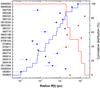 |
Fig. 1 Shown here are lower (to-the-right pointing triangles) and upper (to-the-left pointing triangles) limits on the position of the wind termination shock based on Eq. (1), assuming A ⋆ = 1 in all cases (Table 3). Note that GRB 060614 is a much debated burst (see Sect. 3.1.1). The step curves are the cumulative distributions to the lower limits up to which a wind profile is identified and upper limits after which a constant density medium (ISM) agrees with the data. |
Is the width of the distribution we have found for the upper limits on the wind
termination shock reasonable? Based on numerical wind models of Wolf-Rayet stars, Fryer et al. (2006) found that for
A ⋆ = 1 the radius of the termination
shock is approximately given by  (2)ISM densities of the order of
106 cm-3 are then required to reduce
RT to 0.01 pc. These large-scale gas densities are rather
unique and only typical for dense cores of molecular clouds (with the Rho Ophiuchi Cloud
as an example, e.g., Klose 1986).
(2)ISM densities of the order of
106 cm-3 are then required to reduce
RT to 0.01 pc. These large-scale gas densities are rather
unique and only typical for dense cores of molecular clouds (with the Rho Ophiuchi Cloud
as an example, e.g., Klose 1986).
Observationally, gas densities could only be derived for a few bursts because of the lack of radio data. So far, the highest values are about 600 cm-3 (Frail et al. 2006; Thöne et al. 2010), while the nominal value is about a factor of 100 smaller (Frail et al. 2006). These measurements do not necessarily rule out the model of Fryer et al. (2006). Successful radio observations might have picked out a certain class of GRBs. Furthermore, radio observations are very challenging at early times because the brightness of the afterglow is increasing in the radio bands while the afterglow is already decaying in the optical and X-ray bands (Zhang & Mészáros 2004). Thus, it is difficult to extract information on the direct vicinity of the progenitor. On the other hand, if the average particle density of the circumburst medium is about 1−10 cm-3, then additional mechanisms are required to bring the wind termination-shock radius closer to the star (e.g., van Marle et al. 2006).
The other possibility to reduce RT is to decrease
A ⋆ , since
 (Chevalier
et al. 2004). For example, for
A ⋆ = 0.01 all data points in Fig. 1 would shift along the R-coordinate to
higher values by a factor of 10 (Eq. (1)),
while RT would decrease by the same factor. In this case,
lower circumburst gas densities would be required. This touches upon the question on how
small A ⋆ can be. Studies of WR stars do not
favour values of less than 0.01 in polar directions (Eldridge 2007, his Table 1). Moreover, observations of nearby WR stars do not
show evidence for these low values either (Nugis &
Lamers 2000). However, the majority of nearby WR stars are surely not seen
pole-on, in contrast to GRBs. Therefore, it is difficult to decide if these observational
constraints on WR stars can be applied to GRB progenitors.
(Chevalier
et al. 2004). For example, for
A ⋆ = 0.01 all data points in Fig. 1 would shift along the R-coordinate to
higher values by a factor of 10 (Eq. (1)),
while RT would decrease by the same factor. In this case,
lower circumburst gas densities would be required. This touches upon the question on how
small A ⋆ can be. Studies of WR stars do not
favour values of less than 0.01 in polar directions (Eldridge 2007, his Table 1). Moreover, observations of nearby WR stars do not
show evidence for these low values either (Nugis &
Lamers 2000). However, the majority of nearby WR stars are surely not seen
pole-on, in contrast to GRBs. Therefore, it is difficult to decide if these observational
constraints on WR stars can be applied to GRB progenitors.
On the other hand, the six GRBs that favour a free wind medium (Table B.3) have large lower limits on the wind termination-shock radius (Table 3). This matches theoretical models by van Marle et al. (2007, 2008), which allow RT to extend up to several parsecs.
The separation between the lower and upper limits for wind and ISM-profiles,
respectively, on the wind termination-shock radius could be even larger. Refining the
lower and upper limits is difficult, however. The lower limits, which are deduced from
 (Fig. C.1, Table 3), depend on the observing
strategies due to the brightness of the afterglow and the brightness of the underlying
host galaxy in the optical bands. On the other hand, the upper limits, which are deduced
from
(Fig. C.1, Table 3), depend on the observing
strategies due to the brightness of the afterglow and the brightness of the underlying
host galaxy in the optical bands. On the other hand, the upper limits, which are deduced
from  (Fig. C.1, Table 3), can be affected by
additional radiation components at early times.
(Fig. C.1, Table 3), can be affected by
additional radiation components at early times.
4. Summary and conclusion
After applying several selection criteria (closure relations, the differences in the spectral and temporal slopes, and the flux density ratio, Fopt/Fx) we selected the best-sampled Swift GRBs with well-observed optical as well as X-ray afterglow data from June 2005 to September 2009. Altogether 27 bursts entered our sample, which was used to investigate the density profile of the circumburst medium (constant density medium or free wind), including one short burst (GRB 051221A) and one controversial event in terms of classification (GRB 060614), which successfully passed our selection criteria among all bursts. The other 25 events are classified as long bursts without doubt.
Combining optical with X-ray data is advantageous because optical data usually allow for a more precise determination of the temporal decay slope of an afterglow, while X-ray data can in general be used to extract the SED. Combining both emission components substantially improves our capability to distinguish between an ISM and a wind medium. Thereby, we concentrated on the late-time evolution, i.e., times when the proper afterglow is not affected anymore by flares and additional radiation components (e.g., the reverse shock, central engine activity).
Our study shows that only six of the 25 long bursts (24%) investigated here (GRBs 050603, 070411, 080319B, 080514B, 080916C and 090323) showed evidence for a free wind medium at late times. In the other cases (76%), except for the short burst GRB 051221A and 060904B, the blastwaves were propagating into a constant density-medium. In particular, the controversial burst GRB 060614 favours an ISM profile. This is not in disagreement with a massive-star origin as our result for long bursts indicates.
In addition, we were able to set limits on the wind termination-shock radii of the corresponding GRB progenitors. Only 24 of 27 bursts (Table 3) had good enough data to perform this analysis. Fixing the relative mass-loss rate to A ⋆ = 1, the distribution we deduced covers three orders of magnitude. We find a tentative grouping into (long) GRB progenitors with comparably small and comparably large termination-shock radii. Whether this points to two distinct populations of (long) GRB progenitors or if this is a selection effect, remains an open issue. At least theoretically it is well possible that the long burst population splits into single star progenitors and those belonging to a binary system (Georgy et al. 2009). Further observational data are required to reveal a potential binary nature of the long burst progenitors.
Online material
Appendix A: Smoothly broken power law of the order m
The equation for a smoothly broken power-law of the order m,
Fν,m(t), was derived by
recursion in the following way. Let us assume the function
Fν,m(t) consists of
m power-law segments connected by (m − 1) breaks. To
add an additional power-law segment  , we first normalised the new power-law
segment to the previous one,
Fν,m(t), at the break
time tb,m:
, we first normalised the new power-law
segment to the previous one,
Fν,m(t), at the break
time tb,m: 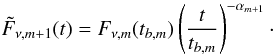 (A.1)Here
αm + 1 is the slope of segment
(m + 1). Second, we followed Beuermann
et al. (1999) and introduced a smoothness
parameter nm so that the smoothly
broken power law of order the (m + 1) takes the form
(A.1)Here
αm + 1 is the slope of segment
(m + 1). Second, we followed Beuermann
et al. (1999) and introduced a smoothness
parameter nm so that the smoothly
broken power law of order the (m + 1) takes the form 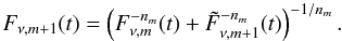 (A.2)If the light-curve consists of
m segments, both steps (adding and smoothing) have to be performed
(m − 1)-times.
(A.2)If the light-curve consists of
m segments, both steps (adding and smoothing) have to be performed
(m − 1)-times.
For example, let us derive the equation for a smoothly broken power-law (Beuermann et al. 1999). In this case
m = 2, thus the function consists of two power-law segments connected
by one break at the time tb,1. The initial
function is a simple power law
Fν,1(t) = C t−α1.
First, the second power-law segment,  , has to be connected to the first one at
the time tb,1 (step A.1)
, has to be connected to the first one at
the time tb,1 (step A.1) 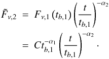 Second, the transition has to be smoothed
by weighting both functions at the point of intersection (step A.2)
Second, the transition has to be smoothed
by weighting both functions at the point of intersection (step A.2) 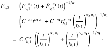 This leads to the equation found by Beuermann et al. (1999) for a smoothly broken
power-law. Repeating both steps leads to a smoothly broken power-law of the order 3
(double smoothly broken power-law; Liang et al.
2008). Thus, looping (m − 1)-times over both steps results in
a smoothly broken power law of the order m.
This leads to the equation found by Beuermann et al. (1999) for a smoothly broken
power-law. Repeating both steps leads to a smoothly broken power-law of the order 3
(double smoothly broken power-law; Liang et al.
2008). Thus, looping (m − 1)-times over both steps results in
a smoothly broken power law of the order m.
Appendix B: Tables
Properties of the afterglow SEDs in the optical and X-ray bands of the 27 bursts that entered our sample.
Light-curve parameters of the late-time optical and X-ray afterglows of the 27 bursts that entered our sample.
Identification of the light-curve segments and the circumburst medium.
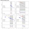 |
Fig. C.1 Optical and X-ray afterglow light curves of the 27 bursts that entered our
sample. Upper panel: the optical data in the
Rc band are shown as dots and the X-ray data at
1.73 keV as bigger dots with an error bar in time. The light-curve fits are
over-plotted. Upper limits are shown as downwards-pointing triangles. The grey box
is the overlapping time interval of the late-time evolution. Vertical dotted and
dashed lines indicate breaks in the optical and X-ray band. Information on the
SEDs are shown in the bottom left (see also Table B.1). The given extinction, |


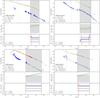 |
Fig. C.1 continued. |
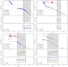 |
Fig. C.1 continued. |
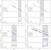 |
Fig. C.1 continued. |
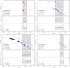 |
Fig. C.1 continued. |
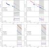 |
Fig. C.1 continued. |
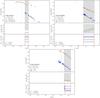 |
Fig. C.1 continued. |
Acknowledgments
We thank the referee for a very careful reading of the manuscript and a rapid reply. S.S. acknowledges support by a Grant of Excellence from the Icelandic Research Fund and Thüringer Landessternwarte Tautenburg, Germany, where part of this study was performed. D.A.K. acknowledges support from grant DFG Kl 766/16-1. A.R. acknowledges support from the BLANCEFLOR Boncompagni-Ludovisi, née Bildt foundation. T.K. acknowledges support by the DFG cluster of excellence “Origin and Structure of the Universe”. S.S. acknowledges Robert Chapman (U Iceland), Elisabetta Maiorano (CNR Bologna), Andrea Mehner (U Minnesota), Kim Page (U Leicester), Eliana Palazzi (CNR Bologna) and Gunnar Stefansson (U Iceland) for helpful discussions. This work made use of data supplied by the UK Swift Science Data Centre at the University of Leicester.
References
- Berger, E., & Becker, G. 2005, GCN Circ., 3520 [Google Scholar]
- Berger, E., Penprase, B. E., Cenko, S. B., et al. 2006, ApJ, 642, 979 [NASA ADS] [CrossRef] [Google Scholar]
- Bessell, M. S. 1979, PASP, 91, 589 [NASA ADS] [CrossRef] [Google Scholar]
- Beuermann, K., Hessman, F. V., Reinsch, K., et al. 1999, A&A, 352, L26 [NASA ADS] [Google Scholar]
- Blinnikov, S. I., Novikov, I. D., Perevodchikova, T. V., & Polnarev, A. G. 1984, SvA Lett., 10, 177 [Google Scholar]
- Bloom, J. S., Foley, R. J., Koceveki, D., & Perley, D. 2006, GCN Circ., 5217 [Google Scholar]
- Bloom, J. S., Perley, D. A., Li, W., et al. 2009, ApJ, 691, 723 [NASA ADS] [CrossRef] [PubMed] [Google Scholar]
- Burrows, D. N., Grupe, D., Capalbi, M., et al. 2006, ApJ, 653, 468 [NASA ADS] [CrossRef] [Google Scholar]
- Butler, N. R., Bloom, J. S., & Poznanski, D. 2010, ApJ, 711, 495 [NASA ADS] [CrossRef] [Google Scholar]
- Castro-Tirado, A. J., Møller, P., García-Segura, G., et al. 2010, A&A, 517, A61 [NASA ADS] [CrossRef] [EDP Sciences] [Google Scholar]
- Cenko, S. B., Frail, D. A., Harrison, F. A., et al. 2010, ApJ, submitted [arXiv:1004.2900] [Google Scholar]
- Cenko, S. B., Kasliwal, M., Harrison, F. A., et al. 2006, ApJ, 652, 490 [NASA ADS] [CrossRef] [Google Scholar]
- Chen, H., Prochaska, J. X., Ramirez-Ruiz, E., et al. 2007, ApJ, 663, 420 [NASA ADS] [CrossRef] [Google Scholar]
- Chevalier, R. A., & Li, Z.-Y. 1999, ApJ, 520, L29 [NASA ADS] [CrossRef] [Google Scholar]
- Chevalier, R. A., & Li, Z.-Y. 2000, ApJ, 536, 195 [NASA ADS] [CrossRef] [Google Scholar]
- Chevalier, R. A., Li, Z.-Y., & Fransson, C. 2004, ApJ, 606, 369 [NASA ADS] [CrossRef] [Google Scholar]
- Chornock, R., Berger, E., Levesque, E. M., et al. 2010, ApJ, submitted [arXiv:1004.2262] [Google Scholar]
- Costa, E., Frontera, F., Heise, J., et al. 1997, Nature, 387, 783 [Google Scholar]
- Crowther, P. A. 2007, ARA&A, 45, 177 [NASA ADS] [CrossRef] [Google Scholar]
- Curran, P. A., Evans, P. A., de Pasquale, M., Page, M. J., & van der Horst, A. J. 2010, ApJ, 716, L135 [NASA ADS] [CrossRef] [Google Scholar]
- Curran, P. A., Starling, R. L. C., van der Horst, A. J., & Wijers, R. A. M. J. 2009, MNRAS, 395, 580 [NASA ADS] [CrossRef] [Google Scholar]
- Dado, S., Dar, A., & De Rújula, A. 2002, A&A, 388, 1079 [NASA ADS] [CrossRef] [EDP Sciences] [Google Scholar]
- de Pasquale, M., Oates, S. R., Page, M. J., et al. 2007, MNRAS, 377, 1638 [NASA ADS] [CrossRef] [Google Scholar]
- de Ugarte Postigo, A., Jakobsson, P., Malesani, D., et al. 2009, GCN Circ., 8766 [Google Scholar]
- D’Elia, V., Fiore, F., Perna, R., et al. 2009, ApJ, 694, 332 [NASA ADS] [CrossRef] [Google Scholar]
- Della Valle, M., Chincarini, G., Panagia, N., et al. 2006a, Nature, 444, 1050 [NASA ADS] [CrossRef] [PubMed] [Google Scholar]
- Della Valle, M., Malesani, D., Bloom, J. S., et al. 2006b, ApJ, 642, L103 [NASA ADS] [CrossRef] [Google Scholar]
- Della Valle, M., Benetti, S., Mazzali, P., et al. 2008, Central Bureau Electronic Telegrams, 1602 [Google Scholar]
- Eichler, D., Livio, M., Piran, T., & Schramm, D. N. 1989, Nature, 340, 126 [NASA ADS] [CrossRef] [Google Scholar]
- Eldridge, J. J. 2007, MNRAS, 377, L29 [NASA ADS] [Google Scholar]
- Evans, P. A., Beardmore, A. P., Page, K. L., et al. 2007, A&A, 469, 379 [NASA ADS] [CrossRef] [EDP Sciences] [Google Scholar]
- Evans, P. A., Beardmore, A. P., Page, K. L., et al. 2009, MNRAS, 397, 1177 [NASA ADS] [CrossRef] [Google Scholar]
- Fatkhullin , T., Gorosabel, J., de Ugarte Postigo, A., et al. 2009, GCN Circ., 9712 [Google Scholar]
- Ferrero, P., Kann, D. A., Zeh, A., et al. 2006, A&A, 457, 857 [NASA ADS] [CrossRef] [EDP Sciences] [Google Scholar]
- Filippenko, A. V. 1997, ARA&A, 35, 309 [NASA ADS] [CrossRef] [Google Scholar]
- Fox, A. J., Ledoux, C., Vreeswijk, P. M., Smette, A., & Jaunsen, A. O. 2008, A&A, 491, 189 [NASA ADS] [CrossRef] [EDP Sciences] [Google Scholar]
- Frail, D. A., Cameron, P. B., Kasliwal, M., et al. 2006, ApJ, 646, L99 [NASA ADS] [CrossRef] [Google Scholar]
- Fryer, C. L., Rockefeller, G., & Young, P. A. 2006, ApJ, 647, 1269 [NASA ADS] [CrossRef] [Google Scholar]
- Fynbo, J. P. U., Watson, D., Thöne, C. C., et al. 2006, Nature, 444, 1047 [NASA ADS] [CrossRef] [PubMed] [Google Scholar]
- Fynbo, J. P. U., Jakobsson, P., Prochaska, J. X., et al. 2009, ApJS, 185, 526 [NASA ADS] [CrossRef] [Google Scholar]
- Gal-Yam, A., Fox, D. B., Price, P. A., et al. 2006, Nature, 444, 1053 [NASA ADS] [CrossRef] [PubMed] [Google Scholar]
- Galama, T. J., Vreeswijk, P. M., van Paradijs, J., et al. 1998, Nature, 395, 670 [NASA ADS] [CrossRef] [Google Scholar]
- Galama, T. J., Tanvir, N., Vreeswijk, P. M., et al. 2000, ApJ, 536, 185 [NASA ADS] [CrossRef] [Google Scholar]
- Gehrels, N., Norris, J. P., Barthelmy, S. D., et al. 2006, Nature, 444, 1044 [NASA ADS] [CrossRef] [PubMed] [Google Scholar]
- Gehrels, N., Barthelmy, S. D., Burrows, D. N., et al. 2008, ApJ, 689, 1161 [NASA ADS] [CrossRef] [Google Scholar]
- Gendre, B., Klotz, A., Palazzi, E., et al. 2010, MNRAS, 405, 2372 [NASA ADS] [Google Scholar]
- Georgy, C., Meynet, G., Walder, R., Folini, D., & Maeder, A. 2009, A&A, 502, 611 [NASA ADS] [CrossRef] [EDP Sciences] [Google Scholar]
- Ghisellini, G., Nardini, M., Ghirlanda, G., & Celotti, A. 2009, MNRAS, 393, 253 [NASA ADS] [CrossRef] [Google Scholar]
- Goodman, J. 1986, ApJ, 308, L47 [NASA ADS] [CrossRef] [Google Scholar]
- Greiner, J., Clemens, C., Krühler, T., et al. 2009a, A&A, 498, 89 [NASA ADS] [CrossRef] [EDP Sciences] [Google Scholar]
- Greiner, J., Krühler, T., Fynbo, J. P. U., et al. 2009b, ApJ, 693, 1610 [NASA ADS] [CrossRef] [Google Scholar]
- Haislip, J., Reichart, D., Cominsky, L., McLin, K., et al. 2009, GCN Circ., 9926 [Google Scholar]
- Hjorth, J., Sollerman, J., Møller, P., et al. 2003, Nature, 423, 847 [NASA ADS] [CrossRef] [PubMed] [Google Scholar]
- Iwamoto, K., Mazzali, P. A., Nomoto, K., et al. 1998, Nature, 395, 672 [NASA ADS] [CrossRef] [Google Scholar]
- Jakobsson, P., Fynbo, J. P. U., Ledoux, C., et al. 2006, A&A, 460, L13 [NASA ADS] [CrossRef] [EDP Sciences] [Google Scholar]
- Kalberla, P. M. W., Burton, W. B., Hartmann, D., et al. 2005, A&A, 440, 775 [NASA ADS] [CrossRef] [EDP Sciences] [Google Scholar]
- Kann, D. A., Klose, S., & Zeh, A. 2006, ApJ, 641, 993 [NASA ADS] [CrossRef] [Google Scholar]
- Kann, D. A., Klose, S., Zhang, B., et al. 2008, ApJ, submitted [arXiv:0804.1959] [Google Scholar]
- Kann, D. A., Klose, S., Zhang, B., et al. 2010, ApJ, 720, 1513 [NASA ADS] [CrossRef] [Google Scholar]
- Kawabata, K. S., Deng, J., Wang, L., et al. 2003, ApJ, 593, L19 [NASA ADS] [CrossRef] [Google Scholar]
- Kelemen, J. 2009, GCN Circ., 10028 [Google Scholar]
- Klose, S. 1986, Ap&SS, 128, 135 [NASA ADS] [CrossRef] [Google Scholar]
- Klose, S., Greiner, J., Rau, A., et al. 2004, AJ, 128, 1942 [NASA ADS] [CrossRef] [Google Scholar]
- Krühler, T., Küpcü Yoldaş, A., Greiner, J., et al. 2008, ApJ, 685, 376 [NASA ADS] [CrossRef] [Google Scholar]
- Krühler, T., Greiner, J., Afonso, P., et al. 2009, A&A, 508, 593 [NASA ADS] [CrossRef] [EDP Sciences] [Google Scholar]
- Kuin, N. P. M., Landsman, W. B., Page, M. J., et al. 2009, MNRAS, 395, L21 [NASA ADS] [Google Scholar]
- Landsman, W. B., & Page, K. 2009, GCN Circ., 9717 [Google Scholar]
- Liang, E., Racusin, J. L., Zhang, B., Zhang, B., & Burrows, D. N. 2008, ApJ, 675, 528 [NASA ADS] [CrossRef] [Google Scholar]
- Malesani, D., Tagliaferri, G., Chincarini, G., et al. 2004, ApJ, 609, L5 [NASA ADS] [CrossRef] [Google Scholar]
- Mangano, V., Holland, S. T., Malesani, D., et al. 2007, A&A, 470, 105 [NASA ADS] [CrossRef] [EDP Sciences] [Google Scholar]
- Masetti, N., Palazzi, E., Pian, E., et al. 2005, A&A, 438, 841 [NASA ADS] [CrossRef] [EDP Sciences] [Google Scholar]
- Matheson, T., Garnavich, P. M., Stanek, K. Z., et al. 2003, ApJ, 599, 394 [NASA ADS] [CrossRef] [Google Scholar]
- McBreen, S., Krühler, T., Rau, A., et al. 2010, A&A, 516, 71 [Google Scholar]
- Mirabal, N., Halpern, J. P., An, D., Thorstensen, J. R., & Terndrup, D. M. 2006, ApJ, 643, L99 [NASA ADS] [CrossRef] [Google Scholar]
- Mirabal, N., Halpern, J. P., Chornock, R., et al. 2003, ApJ, 595, 935 [NASA ADS] [CrossRef] [Google Scholar]
- Modjaz, M., Stanek, K. Z., Garnavich, P. M., et al. 2006, ApJ, 645, L21 [NASA ADS] [CrossRef] [Google Scholar]
- Moretti, A., Campana, S., Mineo, T., et al. 2005, in Presented at the Society of Photo-Optical Instrumentation Engineers (SPIE) Conference, UV, X-Ray, and Gamma-Ray Space Instrumentation for Astronomy XIV, ed. O. H. W. Siegmund, Proc. SPIE, 5898, 360 [Google Scholar]
- Nousek, J. A., Kouveliotou, C., Grupe, D., et al. 2006, ApJ, 642, 389 [NASA ADS] [CrossRef] [Google Scholar]
- Nugis, T., & Lamers, H. J. G. L. M. 2000, A&A, 360, 227 [NASA ADS] [Google Scholar]
- Paczyński, B. 1986, ApJ, 308, L43 [NASA ADS] [CrossRef] [Google Scholar]
- Panaitescu, A. 2007, MNRAS, 380, 374 [NASA ADS] [CrossRef] [Google Scholar]
- Panaitescu, A., & Kumar, P. 2001, ApJ, 560, L49 [NASA ADS] [CrossRef] [Google Scholar]
- Panaitescu, A., & Vestrand, W. T. 2010, MNRAS, submitted [arXiv:1009.3947] [Google Scholar]
- Pe’er, A., & Wijers, R. A. M. J. 2006, ApJ, 643, 1036 [NASA ADS] [CrossRef] [Google Scholar]
- Pian, E., Mazzali, P. A., Masetti, N., et al. 2006, Nature, 442, 1011 [NASA ADS] [CrossRef] [PubMed] [Google Scholar]
- Piranomonte, S., Ward, P. A., Fiore, F., et al. 2008, A&A, 492, 775 [NASA ADS] [CrossRef] [EDP Sciences] [Google Scholar]
- Press, W. H., Teukolsky, S. A., Vetterling, & W. T., Flannery, B. P. 2007, Numerical Recipes, 3rd edn. (Cambridge University Press) [Google Scholar]
- Prochaska, J. X., Chen, H. W., Bloom, J. S., Falco, E., & Dupree, A. K. 2006, GCN Circ., 5002 [Google Scholar]
- Prochaska, J. X., Chen, H., Dessauges-Zavadsky, M., & Bloom, J. S. 2007, ApJ, 666, 267 [NASA ADS] [CrossRef] [Google Scholar]
- Quimby, R., Fox, D., Hoeflich, P., Roman, B., & Wheeler, J. C. 2005, GCN Circ., 4221 [Google Scholar]
- Racusin, J. L., Karpov, S. V., Sokolowski, M., et al. 2008, Nature, 455, 183 [Google Scholar]
- Rau, A., Savaglio, S., Krühler, T., et al. 2010, ApJ, 720, 862 [NASA ADS] [CrossRef] [Google Scholar]
- Reichart, D. E. 1999, ApJ, 521, L111 [NASA ADS] [CrossRef] [Google Scholar]
- Romano, P., Campana, S., Chincarini, G., et al. 2006, A&A, 456, 917 [NASA ADS] [CrossRef] [EDP Sciences] [Google Scholar]
- Rossi, A., de Ugarte Postigo, A., Ferrero, P., et al. 2009, A&A, 491, L29 [Google Scholar]
- Rykoff, E. S., Mangano, V., Yost, S. A., et al. 2006, ApJ, 638, L5 [NASA ADS] [CrossRef] [Google Scholar]
- Sakamoto, T., Donato, D., Gehrels, N., et al. 2009, GCN Circ., 9732 [Google Scholar]
- Sari, R., Piran, T., & Narayan, R. 1998, ApJ, 497, L17 [NASA ADS] [CrossRef] [Google Scholar]
- Schady, P., Mason, K. O., Page, M. J., et al. 2007, MNRAS, 377, 273 [NASA ADS] [CrossRef] [Google Scholar]
- Schady, P., Page, M. J., Oates, S. R., et al. 2010, MNRAS, 401, 2773 [NASA ADS] [CrossRef] [Google Scholar]
- Schaefer, B. E., Gerardy, C. L., Höflich, P., et al. 2003, ApJ, 588, 387 [NASA ADS] [CrossRef] [Google Scholar]
- Shen, R., Kumar, P., & Robinson, E. L. 2006, MNRAS, 371, 1441 [NASA ADS] [CrossRef] [Google Scholar]
- Soderberg, A. M., Kulkarni, S. R., Price, P. A., et al. 2006, ApJ, 636, 391 [NASA ADS] [CrossRef] [Google Scholar]
- Sollerman, J., Kozma, C., Fransson, C., et al. 2000, ApJ, 537, L127 [NASA ADS] [CrossRef] [Google Scholar]
- Sollerman, J., Jaunsen, A. O., Fynbo, J. P. U., et al. 2006, A&A, 454, 503 [NASA ADS] [CrossRef] [EDP Sciences] [Google Scholar]
- Stanek, K. Z., Matheson, T., Garnavich, P. M., et al. 2003, ApJ, 591, L17 [NASA ADS] [CrossRef] [Google Scholar]
- Starling, R. L. C., Wijers, R. A. M. J., Hughes, M. A., et al. 2005, MNRAS, 360, 305 [NASA ADS] [CrossRef] [Google Scholar]
- Starling, R. L. C., van der Horst, A. J., Rol, E., et al. 2008, ApJ, 672, 433 [NASA ADS] [CrossRef] [Google Scholar]
- Starling, R. L. C., Rol, E., van der Horst, A. J., et al. 2009, MNRAS, 400, 90 [NASA ADS] [CrossRef] [Google Scholar]
- Starling, R. L. C., Wiersema, K., Levan, A. J., et al. 2010, MNRAS, in press [arXiv:1004.2919v2] [Google Scholar]
- Tanvir, N. R., Rol, E., Levan, A., et al. 2008, ApJ, 725, 625 [Google Scholar]
- Thöne, C. C., Perley, D. A., Cooke, J., et al. 2007, GCN Circ., 6741 [Google Scholar]
- Thöne, C. C., Kann, D. A., Jóhannesson, G., et al. 2010, A&A, 523, A70 [NASA ADS] [CrossRef] [EDP Sciences] [Google Scholar]
- Šimon, V., Polášek, C., Jelínek, M., Hudec, R., & Trobl, J. Å. 2010, A&A, 510, A49 [NASA ADS] [CrossRef] [EDP Sciences] [Google Scholar]
- van Marle, A. J., Langer, N., Achterberg, A., & García-Segura, G. 2006, A&A, 460, 105 [NASA ADS] [CrossRef] [EDP Sciences] [Google Scholar]
- van Marle, A. J., Langer, N., & García-Segura, G. 2007, A&A, 469, 941 [NASA ADS] [CrossRef] [EDP Sciences] [Google Scholar]
- van Marle, A. J., Langer, N., Yoon, S., & García-Segura, G. 2008, A&A, 478, 769 [NASA ADS] [CrossRef] [EDP Sciences] [Google Scholar]
- van Paradijs, J., Groot, P. J., Galama, T. J., et al. 1997, Nature, 386, 686 [NASA ADS] [CrossRef] [Google Scholar]
- Vaughan, S., Goad, M. R., Beardmore, A. P., et al. 2006, ApJ, 638, 920 [NASA ADS] [CrossRef] [Google Scholar]
- Volnova, A., Pavlenko, E., Sklyanov, A., Antoniuk, O., & Pozanenko, A. 2009, GCN Circ., 9741 [Google Scholar]
- Wilms, J., Allen, A., & McCray, R. 2000, ApJ, 542, 914 [NASA ADS] [CrossRef] [Google Scholar]
- Woosley, S. E., & Bloom, J. S. 2006, ARA&A, 44, 507 [NASA ADS] [CrossRef] [Google Scholar]
- Zeh, A., Klose, S., & Hartmann, D. H. 2004, ApJ, 609, 952 [NASA ADS] [CrossRef] [Google Scholar]
- Zeh, A., Klose, S., & Kann, D. A. 2006, ApJ, 637, 889 [NASA ADS] [CrossRef] [Google Scholar]
- Zhang, B., & Mészáros, P. 2004, Int. J. Mod. Phys. A, 19, 2385 [NASA ADS] [CrossRef] [Google Scholar]
- Zhang, B., Fan, Y. Z., Dyks, J., et al. 2006, ApJ, 642, 354 [NASA ADS] [CrossRef] [Google Scholar]
- Zhang, B., Zhang, B.-B., Liang, E.-W., et al. 2007, ApJ, 655, L25 [NASA ADS] [CrossRef] [Google Scholar]
- Zhang, B., Zhang, B., Virgili, F. J., et al. 2009, ApJ, 703, 1696 [NASA ADS] [CrossRef] [Google Scholar]
All Tables
The closure relations combining the temporal decay slope α and the spectral slope β (adopted from Zhang & Mészáros 2004; and Panaitescu 2007; valid for p > 2).
Properties of the afterglow SEDs in the optical and X-ray bands of the 27 bursts that entered our sample.
Light-curve parameters of the late-time optical and X-ray afterglows of the 27 bursts that entered our sample.
All Figures
|
Fig. 1 Shown here are lower (to-the-right pointing triangles) and upper (to-the-left pointing triangles) limits on the position of the wind termination shock based on Eq. (1), assuming A ⋆ = 1 in all cases (Table 3). Note that GRB 060614 is a much debated burst (see Sect. 3.1.1). The step curves are the cumulative distributions to the lower limits up to which a wind profile is identified and upper limits after which a constant density medium (ISM) agrees with the data. |
| In the text | |
|
Fig. C.1 Optical and X-ray afterglow light curves of the 27 bursts that entered our
sample. Upper panel: the optical data in the
Rc band are shown as dots and the X-ray data at
1.73 keV as bigger dots with an error bar in time. The light-curve fits are
over-plotted. Upper limits are shown as downwards-pointing triangles. The grey box
is the overlapping time interval of the late-time evolution. Vertical dotted and
dashed lines indicate breaks in the optical and X-ray band. Information on the
SEDs are shown in the bottom left (see also Table B.1). The given extinction, |
| In the text | |
|
Fig. C.1 continued. |
| In the text | |
|
Fig. C.1 continued. |
| In the text | |
|
Fig. C.1 continued. |
| In the text | |
|
Fig. C.1 continued. |
| In the text | |
|
Fig. C.1 continued. |
| In the text | |
|
Fig. C.1 continued. |
| In the text | |
Current usage metrics show cumulative count of Article Views (full-text article views including HTML views, PDF and ePub downloads, according to the available data) and Abstracts Views on Vision4Press platform.
Data correspond to usage on the plateform after 2015. The current usage metrics is available 48-96 hours after online publication and is updated daily on week days.
Initial download of the metrics may take a while.