The circumburst density profile around GRB progenitors: a statistical study

Home

All issues

Volume 526 (February 2011)

A&A, 526 (2011) A23

Online Material

Free Access

Issue		A&A Volume 526, February 2011


Article Number		A23
Number of page(s)		20
Section		Extragalactic astronomy
DOI		https://doi.org/10.1051/0004-6361/201015581
Published online		15 December 2010

Online material

Appendix A: Smoothly broken power law of the order m

The equation for a smoothly broken power-law of the order m, F_ν,m(t), was derived by recursion in the following way. Let us assume the function F_ν,m(t) consists of m power-law segments connected by (m − 1) breaks. To add an additional power-law segment , we first normalised the new power-law segment to the previous one, F_ν,m(t), at the break time t_b,m: 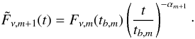(A.1)Here α_m + 1 is the slope of segment (m + 1). Second, we followed Beuermann et al. (1999) and introduced a smoothness parameter n_m so that the smoothly broken power law of order the (m + 1) takes the form 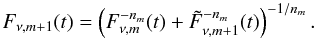(A.2)If the light-curve consists of m segments, both steps (adding and smoothing) have to be performed (m − 1)-times.

For example, let us derive the equation for a smoothly broken power-law (Beuermann et al. 1999). In this case m = 2, thus the function consists of two power-law segments connected by one break at the time t_b,1. The initial function is a simple power law F_ν,1(t) = C t^−α₁. First, the second power-law segment, , has to be connected to the first one at the time t_b,1 (step A.1) 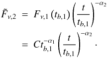Second, the transition has to be smoothed by weighting both functions at the point of intersection (step A.2) This leads to the equation found by Beuermann et al. (1999) for a smoothly broken power-law. Repeating both steps leads to a smoothly broken power-law of the order 3 (double smoothly broken power-law; Liang et al. 2008). Thus, looping (m − 1)-times over both steps results in a smoothly broken power law of the order m.

Appendix B: Tables

Table B.1

Properties of the afterglow SEDs in the optical and X-ray bands of the 27 bursts that entered our sample.

Table B.2

Light-curve parameters of the late-time optical and X-ray afterglows of the 27 bursts that entered our sample.

Table B.3

Identification of the light-curve segments and the circumburst medium.

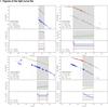Fig. C.1

Optical and X-ray afterglow light curves of the 27 bursts that entered our sample. Upper panel: the optical data in the R_c band are shown as dots and the X-ray data at 1.73 keV as bigger dots with an error bar in time. The light-curve fits are over-plotted. Upper limits are shown as downwards-pointing triangles. The grey box is the overlapping time interval of the late-time evolution. Vertical dotted and dashed lines indicate breaks in the optical and X-ray band. Information on the SEDs are shown in the bottom left (see also Table B.1). The given extinction, , is the observed host-extinction in the R_c band based on the deduced host extinction in the V-band, . Additionally, we deduced the electron index, p, from β_x. The electron index is either p = 2β if ν_c < ν_x or p = 2β + 1 if ν_c > ν_x (e.g., Zhang & Mészáros 2004). Its error was computed by propagating the uncertainty in β_x. Middle panel: the flux density ratio between the optical and X-ray afterglow is shown as a solid line and its error as a dashed line for the shared time interval of the late-time evolution. The grey box represents the allowed parameter space of the flux density ratio (Table 1). The upper boundary is the expected flux density ratio for ν_c ≤ ν_opt, while the lower one shows the expected ratio for ν_c ≥ ν_x. If the cooling break is in between the optical and the X-ray bands, the expected flux-density ratio lies be in between these boundaries. The expected flux density ratio depends on the electron index. Not all bursts could be corrected for host extinction. The error on the electron index was neither propagated into the error of the expected nor of the observed flux-density ratio. Lower panel: the first logarithmic derivative of the flux-density ratio, , is shown as a solid curve and its error is plotted as a dashed line. For t/t_break ≇ 1, the first logarithmic derivative is identical to the difference in the decay slopes obtained from the light-curve fit (asymptotic values). Usually breaks in the light curves tend to be smooth instead of sharp. Because of this, the first logarithmic derivative deviates from the asymptotic value close to a break depending on the smoothness of the break. Two solid lines are plotted to highlight the time interval when the asymptotic decay slopes were reached within 1σ. The precise values are shown on the left and in Table 3. Within 3σ, the asymptotic difference in the decay slopes agrees either with +1/4, 0, −1/4 depending on the spectral and dynamical regime and the circumburst density profile. Furthermore, an envelope is drawn around expected values, +1/4, 0, −1/4, with a width of 0.1 to guide the eye.

Open with DEXTER

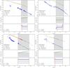	Fig. C.1 continued.
Open with DEXTER

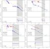	Fig. C.1 continued.
Open with DEXTER

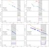	Fig. C.1 continued.
Open with DEXTER

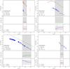	Fig. C.1 continued.
Open with DEXTER

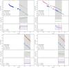	Fig. C.1 continued.
Open with DEXTER

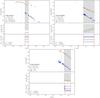	Fig. C.1 continued.
Open with DEXTER

© ESO, 2010

Current usage metrics show cumulative count of Article Views (full-text article views including HTML views, PDF and ePub downloads, according to the available data) and Abstracts Views on Vision4Press platform.

Data correspond to usage on the plateform after 2015. The current usage metrics is available 48-96 hours after online publication and is updated daily on week days.

Initial download of the metrics may take a while.