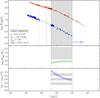
Fig. C.1
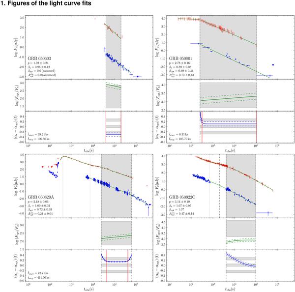
Optical and X-ray afterglow light curves of the 27 bursts that entered our
sample. Upper panel: the optical data in the
Rc band are shown as dots and the X-ray data at
1.73 keV as bigger dots with an error bar in time. The light-curve fits are
over-plotted. Upper limits are shown as downwards-pointing triangles. The grey box
is the overlapping time interval of the late-time evolution. Vertical dotted and
dashed lines indicate breaks in the optical and X-ray band. Information on the
SEDs are shown in the bottom left (see also Table B.1). The given extinction,  , is the observed host-extinction
in the Rc band based on the deduced host extinction in
the V-band,
, is the observed host-extinction
in the Rc band based on the deduced host extinction in
the V-band,  . Additionally, we deduced the
electron index, p, from βx. The
electron index is either p = 2β if
νc < νx or
p = 2β + 1 if
νc > νx (e.g.,
Zhang & Mészáros 2004). Its
error was computed by propagating the uncertainty in βx. Middle
panel: the flux density ratio between the optical and X-ray afterglow
is shown as a solid line and its error as a dashed line for the shared time
interval of the late-time evolution. The grey box represents the allowed parameter
space of the flux density ratio (Table 1).
The upper boundary is the expected flux density ratio for
νc ≤ νopt, while the
lower one shows the expected ratio for
νc ≥ νx. If the cooling
break is in between the optical and the X-ray bands, the expected flux-density
ratio lies be in between these boundaries. The expected flux density ratio depends
on the electron index. Not all bursts could be corrected for host extinction. The
error on the electron index was neither propagated into the error of the expected
nor of the observed flux-density ratio. Lower panel: the first
logarithmic derivative of the flux-density ratio,
. Additionally, we deduced the
electron index, p, from βx. The
electron index is either p = 2β if
νc < νx or
p = 2β + 1 if
νc > νx (e.g.,
Zhang & Mészáros 2004). Its
error was computed by propagating the uncertainty in βx. Middle
panel: the flux density ratio between the optical and X-ray afterglow
is shown as a solid line and its error as a dashed line for the shared time
interval of the late-time evolution. The grey box represents the allowed parameter
space of the flux density ratio (Table 1).
The upper boundary is the expected flux density ratio for
νc ≤ νopt, while the
lower one shows the expected ratio for
νc ≥ νx. If the cooling
break is in between the optical and the X-ray bands, the expected flux-density
ratio lies be in between these boundaries. The expected flux density ratio depends
on the electron index. Not all bursts could be corrected for host extinction. The
error on the electron index was neither propagated into the error of the expected
nor of the observed flux-density ratio. Lower panel: the first
logarithmic derivative of the flux-density ratio,
 , is shown as a solid curve and its
error is plotted as a dashed line. For
t/tbreak ≇ 1, the first logarithmic
derivative is identical to the difference in the decay slopes obtained from the
light-curve fit (asymptotic values). Usually breaks in the light curves tend to be
smooth instead of sharp. Because of this, the first logarithmic derivative
deviates from the asymptotic value close to a break depending on the smoothness of
the break. Two solid lines are plotted to highlight the time interval when the
asymptotic decay slopes were reached within 1σ. The precise
values are shown on the left and in Table 3. Within 3σ, the asymptotic difference in the decay
slopes agrees either with +1/4, 0, −1/4 depending on the spectral and dynamical
regime and the circumburst density profile. Furthermore, an envelope is drawn
around expected values, +1/4, 0, −1/4, with a width of 0.1 to guide the eye.
, is shown as a solid curve and its
error is plotted as a dashed line. For
t/tbreak ≇ 1, the first logarithmic
derivative is identical to the difference in the decay slopes obtained from the
light-curve fit (asymptotic values). Usually breaks in the light curves tend to be
smooth instead of sharp. Because of this, the first logarithmic derivative
deviates from the asymptotic value close to a break depending on the smoothness of
the break. Two solid lines are plotted to highlight the time interval when the
asymptotic decay slopes were reached within 1σ. The precise
values are shown on the left and in Table 3. Within 3σ, the asymptotic difference in the decay
slopes agrees either with +1/4, 0, −1/4 depending on the spectral and dynamical
regime and the circumburst density profile. Furthermore, an envelope is drawn
around expected values, +1/4, 0, −1/4, with a width of 0.1 to guide the eye.
Current usage metrics show cumulative count of Article Views (full-text article views including HTML views, PDF and ePub downloads, according to the available data) and Abstracts Views on Vision4Press platform.
Data correspond to usage on the plateform after 2015. The current usage metrics is available 48-96 hours after online publication and is updated daily on week days.
Initial download of the metrics may take a while.