| Issue |
A&A
Volume 526, February 2011
|
|
|---|---|---|
| Article Number | A65 | |
| Number of page(s) | 12 | |
| Section | Stellar structure and evolution | |
| DOI | https://doi.org/10.1051/0004-6361/201015571 | |
| Published online | 22 December 2010 | |
Low-frequency internal waves in magnetized rotating stellar radiation zones
I. Wave structure modification by a toroidal field
1
Laboratoire AIM, CEA/DSM – CNRS – Université Paris Diderot,
IRFU/SAp Centre de Saclay,
91191
Gif-sur-Yvette,
France
e-mail: This email address is being protected from spambots. You need JavaScript enabled to view it.
, This email address is being protected from spambots. You need JavaScript enabled to view it.
2
LESIA, Observatoire de Paris – CNRS – Université Paris Diderot,
Place Jules Janssen,
92195
Meudon,
France
Received:
11
August
2010
Accepted:
23
September
2010
Abstract
Context. The study of helioseismology, asteroseismology, and powerful ground-based instrumentation dedicated to stellar physics is developing strongly (cf. CoRoT, KEPLER, and ESPaDOnS). This generates tight constraints on the stellar internal structure and dynamical processes. In this context, it is thus necessary to go beyond the non-rotating and the non-magnetic picture of stellar interiors, particularly for large-scale transport mechanisms and waves.
Aims. We focus on low-frequency internal waves in magnetic, rotating, stably stratified stellar radiation zones. For frequencies, which can be close to the Alfvén and the inertial frequencies, we go beyond the non-magnetic and non-rotating description of wave dynamics with taking the Coriolis acceleration and the Lorentz force into account. Then, we have to couple wave dynamics with fossil magnetic fields, which must have mixed configurations (both poloidal and toroidal) to survive in stellar radiation zones.
Methods. We chose to study such coupling step by step, first with purely toroidal fields and then with purely poloidal fields, to unravel their modification by each corresponding component of a realistic mixed-field. Thus, we analytically built a complete formalism, which describes both effects of the Coriolis acceleration and of the Lorentz force in a non-perturbative way in the case of an axisymmetric toroidal field. We consider here the case where both Alfvén frequency and angular velocity are chosen to be uniform, to isolate wave properties.
Results. The different approximations possible for low-frequency internal waves in this model are examined and discussed. In this way, the traditional approximation used to describe the dynamics of low-frequency regular elliptic gravito-inertial waves in the purely hydrodynamical case is generalized to the magnetic one. The complete structure of internal waves, which become magneto-gravito-inertial waves, is then derived and compared to the non-magnetic case. The asymptotic behaviour of such waves is obtained.
Conclusions. A global study of magneto-gravito-inertial waves in stellar radiation zones is achieved in the case of an axisymmetric toroidal magnetic field. In the near future, consequences for angular momentum transport and the case of general differential rotation and azimuthal magnetic field have to be studied. Moreover, the same methodology must be applied to the case of poloidal fields, and the hyperbolic regime has to be carefully studied.
Key words: magnetohydrodynamics (MHD) / waves / methods: analytical / stars: rotation / stars: magnetic field / stars: oscillations
© ESO, 2010
1. Introduction
Stellar radiation zones are stable strongly stratified rotating magnetic regions. This means that fluid dynamics in such zones are driven by the buoyancy force, the Coriolis and the centrifugal accelerations, and the Lorentz force. Furthermore, those regions are the seat of transport and mixing processes that rule the secular evolution of stars along with nuclear reactions (see for example Zahn 1992; Meynet & Maeder 2000). Then, angular momentum, heat, magnetic field, and chemicals are transported, leading to a modification of the stellar structure.
Observations from space and ground (with helioseismology, asteroseismology, and high-resolution spectropolarimetry, for example) now give us ever more refined constraints on physical processes in star interiors. In this way, we have to built models that become more and more realistic, now taking internal dynamical processes into account. A complete review of those mechanisms in stellar radiation zones is given by Talon (2008).
In this work, we focus on the waves that propagate in such regions, namely the internal (or gravity) waves. These waves transport angular momentum along with fossil magnetic field (Mestel et al. 1988; Gough & McIntyre 1998; Brun & Zahn 2006; Garaud & Guervilly 2009) and are serious candidates for explaining stellar radiation zone angular velocity profiles, as in the Sun and solar-type stars (cf. Talon et al. 2002; Talon & Charbonnel 2005; Charbonnel & Talon 2005; Denissenkov et al. 2008). Since stellar radiation regions are differentially rotating and magnetic (for example, in the solar tachocline where waves are excited; see Browning et al. 2006), internal waves dynamics are modified by the Coriolis acceleration (the centrifugal one can be neglected to the first order in rotation) and by the Lorentz force, thus becoming magneto-gravito-inertial waves (Schatzman 1993a; Barnes et al. 1998; Kumar et al. 1999; Schecter et al. 2001; Rogers & MacGregor 2010). They are equivalent to the MAC waves (for magnetic-Archimedean-Coriolis) studied in geophysics for the liquid Earth’s core (see Braginsky 1967; Braginsky & Roberts 1975; Friedlander 1987b, 1989), but the relative importance of each force is however different in the stellar case with a strong domination of the stratification restoring force. For the fossil magnetic field configuration in stellar radiation zones, the simplest geometrical configurations, such as purely poloidal and purely toroidal fields, are known to be unstable (Tayler 1973; Achesson 1978; Markey & Tayler 1973, 1974), with the best candidate for stable geometries the mixed poloidal-toroidal fields (Wright 1973; Markey & Tayler 1974; Tayler 1980; Braithwaite & Spruit 2004; Braithwaite 2009; Duez & Mathis 2010). However, it is a hard and very new task to consider such a complex helical field geometry in the study of internal wave dynamics. This is the reason we chose to treat the modification of wave propagation, and the transport they induce, first by a purely toroidal field, and second by a purely poloidal field (see for example Lee 2005-2007-2010 in the dipolar case), to unravel their modification by each corresponding component of a realistic mixed field.
The wave dynamics equations are given here for an axisymmetric toroidal (and thus azimuthal) magnetic field in Sect. 2. Examining a model of rotating and magnetic stellar radiation zone where the angular velocity and the Alfvén frequency are assumed to be uniform (cf. Fig. 1), which constitutes the first step in understanding the complex behaviour of such waves, we introduce in Sect. 3 the so-called traditional approximation, which we generalize to the MHD case. In this framework, we derive the complete spatial structure of magneto-gravito-inertial waves and their asymptotic properties. Then, the validity of the MHD traditional approximation is discussed in Sect. 4 and wave families are identified. Finally, conclusions are given and perspectives for modifying wave-induced transport of angular momentum are discussed in Sect. 5.
2. Waves in rotating stars with a toroidal magnetic field
To study the dynamics of magneto-gravito-inertial waves in stellar radiation zones, the
classical perfect MHD inviscid dynamical equations system has to be solved. It is formed by
the induction equation in the non-dissipative case (here, the ohmic dissipation is not taken
into account because it is negligible compared to the thermal diffusion)  (1)the momentum equation
![Mathematical equation: \begin{equation} D_{t}\vec V=-\frac{1}{\rho}\vec\nabla P-\vec\nabla\Phi+\frac{1}{\rho}\left[\frac{1}{\mu}\left(\vec\nabla\times\vec B\right)\times\vec B\right], \label{eqd2} \end{equation}](/articles/aa/full_html/2011/02/aa15571-10/aa15571-10-eq2.png) (2)the continuity
equation
(2)the continuity
equation  (3)the equation for the
energy transport, which is given here in the adiabatic limit
(3)the equation for the
energy transport, which is given here in the adiabatic limit  (4)and the Poisson’s
equation for the gravitational potential
(4)and the Poisson’s
equation for the gravitational potential  (5)Here,
B is the macroscopic magnetic field. It is formed by the
sum of the large-scale toroidal field
(5)Here,
B is the macroscopic magnetic field. It is formed by the
sum of the large-scale toroidal field  ,
associated to the chosen uniform Alfvén frequency ωA1, and of the wave-induced magnetic field
b:
,
associated to the chosen uniform Alfvén frequency ωA1, and of the wave-induced magnetic field
b:  (6)where
t is the time and
r = (r,θ,ϕ) are the usual spherical
coordinates with their associated unit vector basis
(6)where
t is the time and
r = (r,θ,ϕ) are the usual spherical
coordinates with their associated unit vector basis  ,
ρ is the density, and μ is the magnetic permeability of
the medium. Next, V is the macroscopic velocity field. It is
formed by the sum of the large-scale azimuthal velocity
V0, associated to the chosen uniform rotation
Ωs, and of the wave velocity u:
,
ρ is the density, and μ is the magnetic permeability of
the medium. Next, V is the macroscopic velocity field. It is
formed by the sum of the large-scale azimuthal velocity
V0, associated to the chosen uniform rotation
Ωs, and of the wave velocity u:  (7)where
Dt = ∂t + (V·∇)
is the Lagrangian derivative. The Φ and P are the gravitational potential
and the pressure, while
Γ1 = (∂lnP/∂lnρ)S
is the adiabatic exponent, with S the macroscopic entropy, and
G the universal gravitational constant.
(7)where
Dt = ∂t + (V·∇)
is the Lagrangian derivative. The Φ and P are the gravitational potential
and the pressure, while
Γ1 = (∂lnP/∂lnρ)S
is the adiabatic exponent, with S the macroscopic entropy, and
G the universal gravitational constant.
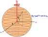 |
Fig. 1 The set-up to study internal wave dynamics in rotating and magnetic stellar radiation
zones. Angular velocity (Ωs) and Alfvén frequency
|
To achieve our aim, Eqs. (1)–(5) are linearized around the rotating magnetic
steady state. Each scalar field X (the density, the gravitational
potential, and the pressure) is then expanded as the sum of its hydrostatic value
 and of the wave’s
associated fluctuation
and of the wave’s
associated fluctuation  :
:
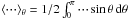
 (8)We neglect the
non-spherical character of the hydrostatic background due to the deformation associated to
the centrifugal acceleration,
(8)We neglect the
non-spherical character of the hydrostatic background due to the deformation associated to
the centrifugal acceleration, ![Mathematical equation: \hbox{$\vec\gamma_{\rm c}\left(\Omega_{\rm s}\right)=1/2\left[\Omega_{\rm s}^{2}\vec\nabla\left(r^2\sin^2\theta\right)\right]$}](/articles/aa/full_html/2011/02/aa15571-10/aa15571-10-eq33.png) , and
to the Lorentz force associated to ,
, and
to the Lorentz force associated to ,
![Mathematical equation: \hbox{${\vec F}_{\mathcal L}^{\,\,0}\left(\vec B_{0}^{\rm T}\right)=1/\mu\left[\left(\vec\nabla\times{\vec B}_{0}^{\rm T}\right)\times{\vec B}_{0}^{\rm T}\right]$}](/articles/aa/full_html/2011/02/aa15571-10/aa15571-10-eq34.png) .
.
Then, following Braginsky (1967), Braginsky &
Roberts (1975), and Unno et al. (1989), the wave’s Lagrangian displacement ξ
is introduced and defined such that  (9)Using Eq. (7), it becomes
 (10)Next, inserting
Eq. (9) in the induction equation
(Eq. (1)), we get
(10)Next, inserting
Eq. (9) in the induction equation
(Eq. (1)), we get
 (11)Using the definition of
given in Eq. (6), this leads to
(11)Using the definition of
given in Eq. (6), this leads to  (12)Then, the momentum
equation (Eq. (2)) becomes
(12)Then, the momentum
equation (Eq. (2)) becomes ![Mathematical equation: \begin{eqnarray} &&\left(\partial_{t}+\Omega_{\rm s}\,\partial_{\varphi}\right)\left[\left(\partial_{t}+\Omega_{\rm s}\,\partial_{\varphi}\right)\vec\xi+2\,\Omega_{\rm s}\,{\widehat{\vec{e}}}_{z}\times\vec\xi\right]= \nonumber\\ \label{momen}&&-\frac{1}{\overline\rho}\vec\nabla\,\Pi\left(\vec r,t\right)-\vec\nabla\,\widetilde\Phi+\frac{\widetilde \rho}{{\overline\rho}^{2}}\vec\nabla\,\overline P+\frac{\vec F_{\mathcal L}^{\,\,{\rm Te}}\left(\vec \xi\right)}{\overline\rho} , \end{eqnarray}](/articles/aa/full_html/2011/02/aa15571-10/aa15571-10-eq40.png) (13)where
(13)where
 is the unit vector along
the rotation axis. Next, the wave total pressure fluctuation is given by the sum of the gas
pressure fluctuation
is the unit vector along
the rotation axis. Next, the wave total pressure fluctuation is given by the sum of the gas
pressure fluctuation  and of the wave magnetic pressure
  :
:
 (14)Afterwards, the wave
magnetic tension force is given by
(14)Afterwards, the wave
magnetic tension force is given by ![Mathematical equation: \begin{eqnarray} \vec F_{\mathcal L}^{\,\,{\rm Te}}\left(\vec \xi\right)&=&\frac{1}{\mu}\left[\left(\vec B_{0}^{\rm T}\cdot\vec\nabla\right)\vec b+\left(\vec b\cdot\vec\nabla\right)\vec B_{0}^{\rm T}\right] \nonumber\\ \label{FLTe}&=&{\overline\rho}\omega_{\rm A}^{2}\left[\partial_{\varphi^2}\vec\xi+2\,{\widehat {\vec e}}_{z}\times\partial_{\varphi}\,\vec\xi\right] . \end{eqnarray}](/articles/aa/full_html/2011/02/aa15571-10/aa15571-10-eq45.png) (15)Finally,
the continuity (Eq. (3)), the energy
transport (Eq. (4)), and the Poisson’s
(Eq. (5)) equations are respectively given
by
(15)Finally,
the continuity (Eq. (3)), the energy
transport (Eq. (4)), and the Poisson’s
(Eq. (5)) equations are respectively given
by  (16)
(16) (17)
(17) (18)Next,
and each vectorial field
x(r,t) = {u,ξ,b}
are expanded in Fourier’s series in ϕ and t:
(18)Next,
and each vectorial field
x(r,t) = {u,ξ,b}
are expanded in Fourier’s series in ϕ and t:
 (19)
(19) (20)with σ the
wave angular velocities in an inertial frame excited in the star.
(20)with σ the
wave angular velocities in an inertial frame excited in the star.
On one hand, we get for the velocity field  (21)In the considered
rotating stellar radiation zone, waves are thus Doppler-shifted by rotation (Ωs)
and the local wave angular velocity
(21)In the considered
rotating stellar radiation zone, waves are thus Doppler-shifted by rotation (Ωs)
and the local wave angular velocity  that
corresponds to the operator
∂t + Ωs∂ϕ
appears.
that
corresponds to the operator
∂t + Ωs∂ϕ
appears.
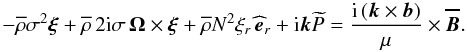
On the other hand, Eq. (12) becomes
 (22)Then, the momentum
equation is written as
(22)Then, the momentum
equation is written as  (23)where
 (24)Expanding each component
explicitely gives along
(24)Expanding each component
explicitely gives along  ,
,
 , and
, and

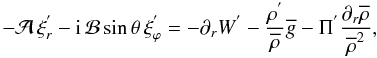 (25)
(25)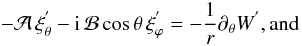 (26)
(26)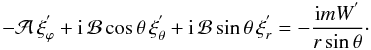 (27)Here
 can be seen as a modified local wave angular velocity that corresponds to the modification
of σs by the presence of the magnetic field. Thus, waves are
only propagating if
can be seen as a modified local wave angular velocity that corresponds to the modification
of σs by the presence of the magnetic field. Thus, waves are
only propagating if  ;
in the other case, they are trapped in the vertical direction (cf. Schatzman 1993a; and Barnes et al. 1998) because the azimuthal magnetic field acts as a filter in this direction (see
in Figs. 6 and 7).
Moreover, we define
;
in the other case, they are trapped in the vertical direction (cf. Schatzman 1993a; and Barnes et al. 1998) because the azimuthal magnetic field acts as a filter in this direction (see
in Figs. 6 and 7).
Moreover, we define 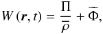 (28)which is the sum of
the total wave dynamical pressure fluctuation2 and of
the gravific potential fluctuation.
(28)which is the sum of
the total wave dynamical pressure fluctuation2 and of
the gravific potential fluctuation.
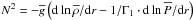
Next, the continuity equation is given by ![Mathematical equation: \begin{equation} \rho^{'}+\frac{1}{r^2}\partial_{r}\left(r^2{\overline\rho}\,\xi_{r}^{'}\right)+\frac{{\overline\rho}}{r}\left[\frac{1}{\sin\theta}\partial_{\theta}\left(\sin\theta\,{\xi}_{\theta}^{'}\right)+\frac{{\rm i} m \xi_{\varphi}^{'}}{\sin\theta}\right]=0 . \label{eqcf} \end{equation}](/articles/aa/full_html/2011/02/aa15571-10/aa15571-10-eq70.png) (29)Afterwards, the
adiabatic energy transport equation becomes
(29)Afterwards, the
adiabatic energy transport equation becomes 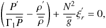 (30)where the gravity
and the Brunt-Väisälä frequency are given by
(30)where the gravity
and the Brunt-Väisälä frequency are given by  and
and
 ,
respectively.
,
respectively.
Finally, the Poisson’s equation is written as
![Mathematical equation: \begin{equation} \frac{1}{r^2}\partial_{r}\left(r^2\partial_{r}\Phi^{'}\right)+\frac{1}{r^2}\left[\frac{1}{\sin\theta}\partial_{\theta}\left(\sin\theta\partial_{\theta}\Phi^{'}\right)-\frac{m^2}{\sin^2\theta}\Phi^{'}\right]=4\pi G \rho^{'} . \end{equation}](/articles/aa/full_html/2011/02/aa15571-10/aa15571-10-eq74.png) (31)From now on, we
adopt the Cowling’s approximation (Cowling 1941)
where the wave’s gravific potential fluctuation
(31)From now on, we
adopt the Cowling’s approximation (Cowling 1941)
where the wave’s gravific potential fluctuation  is
neglected. Therefore, Eq. (28) reduces to
is
neglected. Therefore, Eq. (28) reduces to
 .
.
2.1. Local analysis
Following Kumar et al. (1999) who studied the
dynamics of low-frequency magneto-gravito-inertial waves (cf. Appendix A), we now consider
a more simplified set-up than ours to obtain their dispersion relation. Indeed, we
consider a stellar radiation zone where both the angular velocity and the background
magnetic field are uniform (i.e. Ω = Ωs and
 ).
Then, assuming that all the perturbed quantities have a dependence proportional to
exp[i(k·r + σt)],
the momentum equation (Eq. (2)) becomes
).
Then, assuming that all the perturbed quantities have a dependence proportional to
exp[i(k·r + σt)],
the momentum equation (Eq. (2)) becomes
 (32)After vectorial
manipulations given in Appendix A, this yields to the dispersion relation for waves in
this set-up (Eq. (A.6)):
(32)After vectorial
manipulations given in Appendix A, this yields to the dispersion relation for waves in
this set-up (Eq. (A.6)):
![Mathematical equation: \begin{eqnarray} &&\left[\sigma^2-\left({\vec{\widehat{B}}}\cdot{\vec{k}}\right)^2V_{\rm A}^2\right]^2-\left(\vec N\times{\vec{\widehat{k}}}\right)^2\left[\sigma^2-\left({\vec{\widehat{B}}}\cdot{\vec{k}}\right)^2V_{\rm A}^2\right] \nonumber\\ &-&4\sigma^2\left(\vec\Omega\cdot\vec{\widehat{k}}\right)^2=0 , \end{eqnarray}](/articles/aa/full_html/2011/02/aa15571-10/aa15571-10-eq81.png) (33)where
(33)where
 ,
,
 ,
,
 , and
, and
 . This
can be solved, leading to
. This
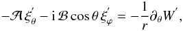
can be solved, leading to ![Mathematical equation: \begin{eqnarray} \sigma^2&=&\left({\vec{\widehat{B}}}\cdot\vec k\right)^2V_{\rm A}^{2}+ \frac{1}{2}\left\{\left(\vec N\times\vec{\widehat{k}}\right)^2+4\left(\vec\Omega\cdot{\vec{\widehat{k}}}\right)^2\right. \nonumber\\[2mm] & \pm&{\left.\sqrt{\left[\left(\vec N\times\vec{\widehat{k}}\right)^2+4\left(\vec\Omega\cdot{\vec{\widehat{k}}}\right)^2\right]^2+16\left(\vec{\widehat{B}}\cdot{\vec k}\right)^2V_{\rm A}^{2}\left(\vec\Omega\cdot{\vec{\widehat{k}}}\right)^2}\,\right\}} . \end{eqnarray}](/articles/aa/full_html/2011/02/aa15571-10/aa15571-10-eq86.png) (34)Let
us now discuss this dispersion relation as done by Heng & Spitkovsky (2009). First, if we examine the non-rotating limit
(Ωs = 0), we get
(34)Let
us now discuss this dispersion relation as done by Heng & Spitkovsky (2009). First, if we examine the non-rotating limit
(Ωs = 0), we get ![Mathematical equation: \begin{equation} \sigma^2= \left\{\begin{array}{l} \left({\vec{\widehat{B}}}\cdot\vec k\right)^2V_{\rm A}^{2}\\[2mm] \left(\vec N\times\vec{\widehat{k}}\right)^2+\left({\vec{\widehat{B}}}\cdot\vec k\right)^2V_{\rm A}^{2} \end{array}.\right. \end{equation}](/articles/aa/full_html/2011/02/aa15571-10/aa15571-10-eq88.png) (35)Two
branches are then isolated: the low-frequency one corresponds to Alfvén waves while
magneto-gravity waves, for which restoring forces are both buoyancy and Lorentz forces,
are linked to the higher-frequency branch (see Schecter et al. 2001).
(35)Two
branches are then isolated: the low-frequency one corresponds to Alfvén waves while
magneto-gravity waves, for which restoring forces are both buoyancy and Lorentz forces,
are linked to the higher-frequency branch (see Schecter et al. 2001).
Then, if we examine the rotating system, both wave families couple through the Coriolis
acceleration. On one hand, for low-frequency Alfvén waves, Coriolis acceleration tries to
balance the Lorentz force and for this reason, those waves are then called
“magnetostrophic waves”. Their approximate dispersion relation is given by
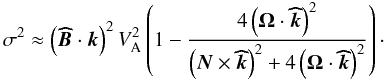 (36)On the other hand,
magneto-gravity waves become magneto-gravito-inertial waves, which are also called
magneto-Poincaré waves and magneto-Rossby waves for those waves that are due to the star
curvature and the associated variation of the local rotation on a tangent sphere. In this
case, we obtain the following approximative dispersion relation:
(36)On the other hand,
magneto-gravity waves become magneto-gravito-inertial waves, which are also called
magneto-Poincaré waves and magneto-Rossby waves for those waves that are due to the star
curvature and the associated variation of the local rotation on a tangent sphere. In this
case, we obtain the following approximative dispersion relation:
![Mathematical equation: \begin{eqnarray} \sigma^2&\approx&\left(\vec N\times{\vec{\widehat{k}}}\right)^{2}+4({\vec \Omega}\cdot{\vec{\widehat{k}}})^2 \nonumber\\[2mm] &&+\left({\vec{\widehat{B}}}\cdot{\vec{k}}\right)^2 V_{\rm A}^{2}\left(1+\frac{4\left(\vec\Omega\cdot{\vec{\widehat{k}}}\right)^2}{\left(\vec N\times{\vec{\widehat{k}}}\right)^2+4\left(\vec\Omega\cdot{\vec{\widehat{k}}}\right)^2}\right)\cdot \end{eqnarray}](/articles/aa/full_html/2011/02/aa15571-10/aa15571-10-eq90.png) (37)Let
us introduce the expansion of k both in the spherical and
cylindrical coordinates:
(37)Let
us introduce the expansion of k both in the spherical and
cylindrical coordinates:  (38)where
 and
and
 , with
(s,ϕ,z) the cylindrical coordinates and
, with
(s,ϕ,z) the cylindrical coordinates and
 the
associated unit-vector basis. Then, the dispersion relation is written as
the
associated unit-vector basis. Then, the dispersion relation is written as
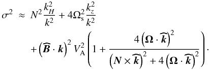 (39)In
the case of highly stratified stellar radiation zones where
ωA ≪ N and
2Ωs ≪ N, this reduces for low-frequency waves
(σ ≪ N) to
(39)In
the case of highly stratified stellar radiation zones where
ωA ≪ N and
2Ωs ≪ N, this reduces for low-frequency waves
(σ ≪ N) to
 (40)which leads to
the following hierarchy
(40)which leads to
the following hierarchy  (41)because of the
anelastic approximation
(41)because of the
anelastic approximation  where acoustic waves are
filtered, which becomes in the local analysis case
k·ξ ≈ 0.
where acoustic waves are
filtered, which becomes in the local analysis case
k·ξ ≈ 0.
From now on, we focus on this type of wave (in the case where ωA ≪ N and 2Ωs ≪ N) for which σ can be of the same order of magnitude as ωA and 2Ωs, and the ratio ωA/2Ωs is taken as general as possible (see Fig. 2 below).
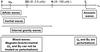 |
Fig. 2 Wave types in a rotating and magnetic stellar radiation zone and associated frequencies (where fL is the Lamb’s frequency). Values for the Sun (⊙ ) at the bottom of the Tachocline are given in brackets. |
3. Low-frequency waves in rotating magnetic stellar radiation zones
3.1. The traditional approximation
We first discuss the non-magnetic case, namely the gravito-inertial waves. In the general case, the Poincaré operator, which governs the spatial structure of waves, is of mixed type (elliptic and hyperbolic) and not separable (see the detailed discussions in Friedlander & Siegman 1982; Dintrans et al. 1999; Dintrans & Rieutord 2000). This leads to the appearance of detached shear layers associated with the underlying singularities of the adiabatic problem that could be crucial for transport and mixing processes in stellar radiation zones, since they are the seat of strong dissipation (cf. Stewartson & Richard 1969; Stewartson & Walton 1976; Dintrans et al. 1999; and Dintrans & Rieutord 2000).
Let us now focus on the case of a uniform rotation (Ω = Ωs). In the largest
part of stellar radiation zones, we are in a regime where
2Ωs ≪ N. Since we are interested here in low-frequency waves
(σ ≪ N), the traditional approximation (hereafter TA),
which consists in neglecting the latitudinal component of the rotation vector
( ),
),
 , in the Coriolis
acceleration, can be adopted in the super-inertial regime where
2Ωs < σ ≪ N (see
e.g. Eckart 1960; for a modern description in a
stellar context see Bildsten et al. 1996; Lee
& Saio 1997; and Mathis et al. 2008). Then, variable separation in radial and
horizontal eigenfunctions remains possible (cf. Friedlander 1987a), which corresponds to the ergodic (regular) elliptic
gravito-inertial mode family (the E1 modes in Dintrans et al. 1999; and Dintrans & Rieutord 2000). This approximation has to be carefully used
however, because it changes the nature of the Poincaré operator, and removes the
singularities and associated shear layers that appear. Then, in the subinertial regime,
where σ ≤ 2Ωs, which corresponds to the equatorially trapped
hyperbolic modes (the H2 modes in Dintrans et al. 1999; and Dintrans & Rieutord 2000), the TA fails to reproduce the waves behaviour and the complete momentum
equation has to be solved (see detailed examples in Gerkema & Shrira 2005; and Gerkema et al. 2008). Note also the work by Fruman (2009), who examines the validity of the TA on the equatorial
β-plane in function of the
2Ωs/N value.
, in the Coriolis
acceleration, can be adopted in the super-inertial regime where
2Ωs < σ ≪ N (see
e.g. Eckart 1960; for a modern description in a
stellar context see Bildsten et al. 1996; Lee
& Saio 1997; and Mathis et al. 2008). Then, variable separation in radial and
horizontal eigenfunctions remains possible (cf. Friedlander 1987a), which corresponds to the ergodic (regular) elliptic
gravito-inertial mode family (the E1 modes in Dintrans et al. 1999; and Dintrans & Rieutord 2000). This approximation has to be carefully used
however, because it changes the nature of the Poincaré operator, and removes the
singularities and associated shear layers that appear. Then, in the subinertial regime,
where σ ≤ 2Ωs, which corresponds to the equatorially trapped
hyperbolic modes (the H2 modes in Dintrans et al. 1999; and Dintrans & Rieutord 2000), the TA fails to reproduce the waves behaviour and the complete momentum
equation has to be solved (see detailed examples in Gerkema & Shrira 2005; and Gerkema et al. 2008). Note also the work by Fruman (2009), who examines the validity of the TA on the equatorial
β-plane in function of the
2Ωs/N value.
As a first step, we thus studied the regular elliptic gravito-inertial waves for which
the TA applies (Mathis et al. 2008; and Mathis
2009). In the MHD case, our purpose is to
generalize the TA to  , thus neglecting the
latitudinal component of
, thus neglecting the
latitudinal component of  since
2Ωs ≪ N,
ωA ≪ N, and
σ ≪ N. Therefore, we restrict ourselves here to the
regular low-frequency waves for which the TA can be used as we show it in the next
section. Its application domain is discussed in Sect. 4.
since
2Ωs ≪ N,
ωA ≪ N, and
σ ≪ N. Therefore, we restrict ourselves here to the
regular low-frequency waves for which the TA can be used as we show it in the next
section. Its application domain is discussed in Sect. 4.
3.2. Dynamical equations
Assuming the TA for low-frequency magneto-gravito-inertial waves, we respectively get for
the linearized momentum equation components: 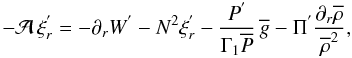 (42)
(42) (43)
(43) (44)where the
linearized energy equation (Eq. (30)) has
been used to express the buoyancy force
(44)where the
linearized energy equation (Eq. (30)) has
been used to express the buoyancy force  .
.
We need to describe the different assumptions for using the TA. On one hand, since
ωA ≪ N and
2Ωs ≪ N, we neglect the
 term
in the radial component of the momentum equation (Eq. (25)). On the other hand, the first term
term
in the radial component of the momentum equation (Eq. (25)). On the other hand, the first term
 also
has to be neglected, but we first conserve it to make the historical link with works in
the non-rotating and non-magnetic cases (Press 1981; Schatzman 1993b; Zahn et al. 1997) and those about gravito-inertial waves (Mathis
et al. 2008; Mathis 2009). Finally, since
also
has to be neglected, but we first conserve it to make the historical link with works in
the non-rotating and non-magnetic cases (Press 1981; Schatzman 1993b; Zahn et al. 1997) and those about gravito-inertial waves (Mathis
et al. 2008; Mathis 2009). Finally, since  (cf. Eq. (41)) for low-frequency internal
waves, the term
(cf. Eq. (41)) for low-frequency internal
waves, the term  is
neglected in the azimuthal component (Eq. (27)).
is
neglected in the azimuthal component (Eq. (27)).
3.3. Spatial structure of the wave-displacement, velocity, and magnetic field
3.3.1. Spatial structure of the horizontal components of the displacement
After successively eliminating  and
and
 between
Eqs. (43) and (44), each of them is expressed in function
of
between
Eqs. (43) and (44), each of them is expressed in function
of ![Mathematical equation: \hbox{$W^{'}=1/{\overline\rho}\left[P^{'}+\left(\vec B_{0}\cdot\vec b^{'}\right)/\mu\right]$}](/articles/aa/full_html/2011/02/aa15571-10/aa15571-10-eq133.png) as
as
![Mathematical equation: \begin{equation} \xi_{\theta}^{'}=\frac{1}{r\,\sigma_{\rm M}^{2}}\frac{1}{\left(1-\nu_{\rm M}^{2}x^{2}\right)\sqrt{1-x^2}}\left[-\left(1-x^2\right)\,\partial_{x}+m\nu_{\rm M}x\right]W^{'} , \label{etathf} \end{equation}](/articles/aa/full_html/2011/02/aa15571-10/aa15571-10-eq134.png) (45)
(45)![Mathematical equation: \begin{equation} \xi_{\varphi}^{'}={\rm i}\frac{1}{r\,\sigma_{\rm M}^{2}}\frac{1}{\left(1-\nu_{\rm M}^{2}x^{2}\right)\sqrt{1-x^2}}\left[-\nu_{\rm M} x\left(1-x^2\right)\,\partial_{x}+m\right]W^{'} , \label{etaphf} \end{equation}](/articles/aa/full_html/2011/02/aa15571-10/aa15571-10-eq135.png) (46)where
x = cosθ has been introduced. Then
νM is defined as
(46)where
x = cosθ has been introduced. Then
νM is defined as
 (47)where
 (48)Here,
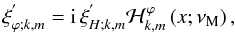
νs is the spin parameter (Fig. 3), which equals the inverse of the Rossby number
Ro = σs/2Ωs
(cf. Lee & Saio 1997), and
FM = νM/νs
gives its modification by the magnetic field.
(48)Here,
νs is the spin parameter (Fig. 3), which equals the inverse of the Rossby number
Ro = σs/2Ωs
(cf. Lee & Saio 1997), and
FM = νM/νs
gives its modification by the magnetic field.
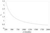 |
Fig. 3 Inverse of the Rossby number (νs) as a function of
the frequency (σ/2π) for
axisymmetric waves |

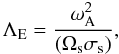
We introduce the wave’s Elsasser number
 (49)which gives the ratio
of the Lorentz force with the Coriolis acceleration (cf. Eqs. (13) and (15) and Fig. 4)3.
(49)which gives the ratio
of the Lorentz force with the Coriolis acceleration (cf. Eqs. (13) and (15) and Fig. 4)3.
 |
Fig. 4 Elsasser number (ΛE) as a function of the wave frequency in the
corotating frame |


3.3.2. Spatial structure of the radial component of the displacement and of the pressure
As in the non-magnetic case and because of the equation structure (cf. Lee &
Saio 1997; Mathis et al. 2008), we choose to expand scalar quantities and the displacement’s
vertical component as 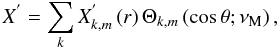 (50)
(50) (51)The
Θk,m functions are the orthogonal Hough functions for
which
(51)The
Θk,m functions are the orthogonal Hough functions for
which  where δ is the Kronecker symbol (Laplace 1799; Hough 1898;
Longuet-Higgins 1968; Lindzen & Chapman
1969). They are the eigenfunctions (with the
associated eigenvalues Λk,m) of the so-called “Laplace tidal
equation” (hereafter LTE):
where δ is the Kronecker symbol (Laplace 1799; Hough 1898;
Longuet-Higgins 1968; Lindzen & Chapman
1969). They are the eigenfunctions (with the
associated eigenvalues Λk,m) of the so-called “Laplace tidal
equation” (hereafter LTE): ![Mathematical equation: \begin{equation} {\mathcal L}_{\nu_{\rm M}}\left[\Theta_{k,m}\left(x;\nu_{\rm M}\right)\right]=-\Lambda_{k,m}\left(\nu_{\rm M}\right)\Theta_{k,m}\left(x;\nu_{\rm M}\right), \label{Laplace} \end{equation}](/articles/aa/full_html/2011/02/aa15571-10/aa15571-10-eq159.png) (52)where the
Laplace tidal operator is given by
(52)where the
Laplace tidal operator is given by
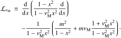 (53)For
a detailed discussion of the boundary conditions of the LTE, we refer the reader to the
Lee & Saio work (1997). Examples of Hough
functions are given in Fig. 5.
(53)For
a detailed discussion of the boundary conditions of the LTE, we refer the reader to the
Lee & Saio work (1997). Examples of Hough
functions are given in Fig. 5.
As emphasized in Mathis et al. (2008), pro and retrograde eigenfunctions (and eigenvalues) are different. This crucial point for induced angular momentum transport will be discussed in detail in Paper II.
 |
Fig. 5 Left: hough functions
Θk,m(cosθ;ν)
(Top) and associated latitudinal
|


This allows separating the radial and latitudinal variables
for and
.
Introducing the amplitude of the horizontal displacement
 leads to
 (54)and the latitudinal
component of ξ′ is written
(54)and the latitudinal
component of ξ′ is written
 (55)where
![Mathematical equation: \begin{equation} {\mathcal H}_{k,m}^{\theta}\left(x;\nu_{\rm M}\right)={\mathcal L}_{\nu_{\rm M};m}^{\theta}\left[\Theta_{k,m}\left(x;\nu_{\rm M}\right)\right] \end{equation}](/articles/aa/full_html/2011/02/aa15571-10/aa15571-10-eq185.png) (56)with
(56)with
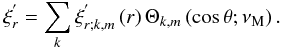
![Mathematical equation: \begin{equation} {\mathcal L}_{\nu_{\rm M};m}^{\theta}\equiv\frac{1}{\left(1-\nu_{\rm M}^{2}x^2\right)\sqrt{1-x^2}}\left[-\left(1-x^2\right)\frac{{\rm d}}{{\rm d}x}+m\nu_{\rm M}x\right] . \end{equation}](/articles/aa/full_html/2011/02/aa15571-10/aa15571-10-eq186.png) (57)In the same way,
its azimuthal component is given by
(57)In the same way,
its azimuthal component is given by
 (58)where
![Mathematical equation: \begin{equation} {\mathcal H}_{k,m}^{\varphi}\left(x;\nu_{\rm M}\right)={\mathcal L}_{\nu_{\rm M};m}^{\varphi}\left[\Theta_{k,m}\left(x;\nu_{\rm M}\right)\right]\ \end{equation}](/articles/aa/full_html/2011/02/aa15571-10/aa15571-10-eq188.png) (59)with
(59)with
![Mathematical equation: \begin{equation} {\mathcal L}_{\nu_{\rm M};m}^{\varphi}\equiv\frac{1}{\left(1-\nu_{\rm M}^{2}x^2\right)\sqrt{1-x^2}}\left[-\nu_{\rm M}x\left(1-x^2\right)\frac{{\rm d}}{{\rm d}x}+m\right] . \end{equation}](/articles/aa/full_html/2011/02/aa15571-10/aa15571-10-eq189.png) (60)Then, the radial
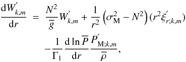
component of the momentum equation assuming the TA (Eq. (42)), the continuity equation (Eq. (29)), and the energy transport equation (Eq. (30)) become
(60)Then, the radial
component of the momentum equation assuming the TA (Eq. (42)), the continuity equation (Eq. (29)), and the energy transport equation (Eq. (30)) become 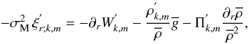 (61)
(61) (62)
(62)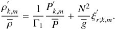 (63)Eliminating
 between the
previous equations and assuming the Cowling’s approximation, we get the following system
for r2ξr;k,m
and
between the
previous equations and assuming the Cowling’s approximation, we get the following system
for r2ξr;k,m
and  :
:
 (64)
(64)![Mathematical equation: \begin{eqnarray} \frac{{\rm d}}{{\rm d}r}\left(r^2\xi_{r;k,m}^{'}\right)&=&\left[\frac{\Lambda_{k,m}\left(\nu_{\rm M}\right)}{\sigma_{\rm M}^{2}}-\frac{{\overline\rho}r^2}{\Gamma_{1}{\overline P}}\right]W_{k,m}^{'}-\frac{1}{\Gamma_{1}{\overline P}}\frac{{\rm d}{\overline P}}{{\rm d}r}\left(r^2\xi_{r;k,m}^{'}\right)\nonumber\\ &&+\frac{r^2}{\Gamma_1{\overline P}}\,P_{{\rm M};k,m}^{'}, \end{eqnarray}](/articles/aa/full_html/2011/02/aa15571-10/aa15571-10-eq197.png) (65)where
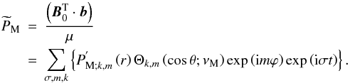
we explicitly introduce the wave magnetic pressure expansion
(65)where
we explicitly introduce the wave magnetic pressure expansion
 (66)Terms
where it explicitly appears are introduced through
(66)Terms
where it explicitly appears are introduced through
 in the
energy equation (Eq. (63)) because of
Eq. (14).
in the
energy equation (Eq. (63)) because of
Eq. (14).
This is a generalization of the system obtained by Press (1981) in the non-rotating and non-magnetic case where
σM and  respectively replace σ and
l(l + 1), where
l is the orbital number of the classical spherical harmonics.
respectively replace σ and
l(l + 1), where
l is the orbital number of the classical spherical harmonics.
Adopting the anelastic approximation, where magneto-acoustic waves are filtered out
(i.e.  and the terms proportional to
 are neglected, where
  is the sound speed), and following the procedure given in Zahn (1970, 1975) and in Press
(1981), we respectively get for the vertical
displacement
is the sound speed), and following the procedure given in Zahn (1970, 1975) and in Press
(1981), we respectively get for the vertical
displacement ![Mathematical equation: \begin{equation} \frac{{\rm d}^{2}{\Psi}_{k,m}}{{\rm d}r^2}\!+\!\left[\left(\frac{N^2}{\sigma_{\rm M}^{2}}-1\right)\!\frac{\Lambda_{k,m}\left(\nu_{\rm M}\right)}{r^2}\!\right]{\Psi}_{k,m}\!=\!0 , \label{Poincare1} \end{equation}](/articles/aa/full_html/2011/02/aa15571-10/aa15571-10-eq207.png) (67)where
(67)where
 ,
and for the pressure fluctuation
,
and for the pressure fluctuation ![Mathematical equation: \begin{equation} \frac{{\rm d}^{2}{\mathcal W}_{k,m}}{{\rm d}r^2}\!+\!\left[\left(\frac{N^2}{\sigma_{\rm M}^{2}}-1\right)\!\frac{\Lambda_{k,m}\left(\nu_{\rm M}\right)}{r^2}\!\right]{\mathcal W}_{k,m}\!=\!0 , \label{Poincare2} \end{equation}](/articles/aa/full_html/2011/02/aa15571-10/aa15571-10-eq209.png) (68)where
(68)where
![Mathematical equation: \hbox{${\mathcal W}_{k,m}=\left[\left({\overline\rho}r^2\right)/N^2\right]^{1/2}W_{k,m}^{'}$}](/articles/aa/full_html/2011/02/aa15571-10/aa15571-10-eq210.png) .
.
3.3.3. The final wave-displacement, velocity, and magnetic field
Once one solves Eq. (67) or Eq. (68), the associated final expression for
ξ, u and
b are derived. First, using Eqs. ((51)−(45)−(46)−(54)), the wave-displacement is given by
![Mathematical equation: \begin{equation} \vec\xi =\sum_{j=\left\{r,\theta,\varphi\right\}}\left[\sum_{\sigma,m,k}\xi_{j;k,m}\right]{\widehat {\vec e}}_{j}, \end{equation}](/articles/aa/full_html/2011/02/aa15571-10/aa15571-10-eq213.png) (69)where
(69)where
 (70)
(70) (71)
(71) (72)Then, the wave
velocity field and magnetic field are straightforwardly derived using
u = i σs ξ
and
(72)Then, the wave
velocity field and magnetic field are straightforwardly derived using
u = i σs ξ
and  (cf. Eqs. (21) and (22)).
Finally, the dynamical pressure is given by  (73)where
 .
.
Therefore, one of the main important conclusions of the study of this model, which
assumes uniform angular velocity (Ωs) and Alfvén frequency
 , is
that the wave-induced perturbations in this case can be completely expressed as a
function of the Hough functions used in the non-magnetic uniformly rotating case. In
that framework, the spin parameter (νs) is now replaced by
νM, which accounts for magnetic field. The simplest case
of magneto-gravity waves is treated in Appendix B.
, is
that the wave-induced perturbations in this case can be completely expressed as a
function of the Hough functions used in the non-magnetic uniformly rotating case. In
that framework, the spin parameter (νs) is now replaced by
νM, which accounts for magnetic field. The simplest case
of magneto-gravity waves is treated in Appendix B.
However, we have to emphasize that such a neat variable separation is not possible in
the case of a general differential rotation and azimuthal magnetic field
(Ω(r,θ),
 ), even
if the TA applies (cf. Mathis 2009). In that
case, which is beyond the scope of the present paper, a more subtle treatment of the
dynamical equations has to be adopted.
), even
if the TA applies (cf. Mathis 2009). In that
case, which is beyond the scope of the present paper, a more subtle treatment of the
dynamical equations has to be adopted.
3.3.4. Asymptotic analysis
Let us now consider the low-frequency waves for which
σ ≪ N. We introduce the vertical wave number
 (74)then, Eq. (67) is written
  (75)For these waves
the J.W.K.B. approximation can be adopted (cf. Landau & Lifshitz 1966; Press 1981; Schatzman 1993b; Zahn et al.
1997). Applying it to Eq. (75), we get4
(75)For these waves
the J.W.K.B. approximation can be adopted (cf. Landau & Lifshitz 1966; Press 1981; Schatzman 1993b; Zahn et al.
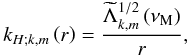
1997). Applying it to Eq. (75), we get4![Mathematical equation: \begin{equation} {\xi}_{r;k,m}^{'}\!=\!E_{k,m}\left(r\right)\exp\left[{\rm i}\,\Phi_{k,m}\left(r\right)\right]~\hbox{with}~\Phi_{k,m}\left(r\right)\!=\!\int_{\,r}^{\,r_{\rm c}}k_{V;k,m}\,{\rm d}r^{'} , \end{equation}](/articles/aa/full_html/2011/02/aa15571-10/aa15571-10-eq225.png) (76)where
rc is the radius of the convection-radiation border while
the amplitude function is given by
(76)where
rc is the radius of the convection-radiation border while
the amplitude function is given by
 (77)Here,
Ak,m is the wave-displacement amplitude
that has to be obtained using excitation models corresponding to the stochastic
excitation by turbulent convective movements (Kiraga et al. 2003, 2005; Dintrans et al.
2005; Rogers & Glatzmaier 2005, 2006;
Belkacem et al. 2009) or to the
κ-mechanism (Lee & Saio 1987; Unno et al. 1989; Lee &
Baraffe 1995).
(77)Here,
Ak,m is the wave-displacement amplitude
that has to be obtained using excitation models corresponding to the stochastic
excitation by turbulent convective movements (Kiraga et al. 2003, 2005; Dintrans et al.
2005; Rogers & Glatzmaier 2005, 2006;
Belkacem et al. 2009) or to the
κ-mechanism (Lee & Saio 1987; Unno et al. 1989; Lee &
Baraffe 1995).
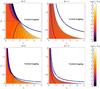 |
Fig. 6 Top: νM as a function of
νs and ΛE for non-axisymmetric retrograde
(m = 1) and prograde (m = −1) waves. The
surfaces such that |νM| = 1 are given by the thick
black lines and the iso-νM lines for
|νM| < 1 and
|νM| > 1 are given by
the red and the blue lines. The big external white region in the top-right corner
in each case corresponds to the |


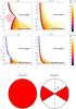 |
Fig. 7 Top: θc as a function of
νs and ΛE for non-axisymmetric retrograde
(m = 1) and prograde (m = −1) waves. As in
Fig. (6), the large white top-right corner
region corresponds to the |
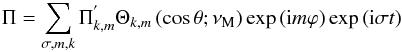
We then derive ξ, u,
b and Π. First, we get
![Mathematical equation: \begin{equation} \vec\xi =\sum_{j}\left[\,\sum_{\sigma,m,k}\xi_{j;k,m}\right]{\widehat {\vec e}}_{j} , \end{equation}](/articles/aa/full_html/2011/02/aa15571-10/aa15571-10-eq241.png) (78)where
(78)where
![Mathematical equation: \begin{eqnarray} \xi_{r;k,m}&=&E_{k,m}\left(r\right)\exp\left[{\rm i}\,\Phi_{k,m}\left(r\right)\right]\nonumber\\ & &\times\,\Theta_{k,m}\left(\cos\theta;\nu_{\rm M}\right)\exp\left({\rm i}m\varphi\right)\exp\left({\rm i}\sigma t\right) , \end{eqnarray}](/articles/aa/full_html/2011/02/aa15571-10/aa15571-10-eq242.png) (79)
(79)![Mathematical equation: \begin{eqnarray} \xi_{\theta;k,m}&=&-{\rm i}\frac{r\,k_{V;k,m}}{\Lambda_{k,m}\left(\nu_{\rm M}\right)}E_{k,m}\left(r\right)\exp\left[{\rm i}\,\Phi_{k,m}\left(r\right)\right]\nonumber\\ & &\times\,{\mathcal H}_{k,m}^{\theta}\left(\cos\theta;\nu_{\rm M}\right)\exp\left({\rm i}m\varphi\right)\exp\left({\rm i}\sigma t\right) , \end{eqnarray}](/articles/aa/full_html/2011/02/aa15571-10/aa15571-10-eq243.png) (80)
(80)![Mathematical equation: \begin{eqnarray} \xi_{\varphi;k,m}&=&\frac{r\,k_{V;k,m}}{\Lambda_{k,m}\left(\nu_{\rm M}\right)}E_{k,m}\left(r\right)\exp\left[{\rm i}\,\Phi_{k,m}\left(r\right)\right]\nonumber\\ & &\times\,{\mathcal H}_{k,m}^{\varphi}\left(\cos\theta;\nu_{\rm M}\right)\exp\left({\rm i}m\varphi\right)\exp\left({\rm i}\sigma t\right) . \end{eqnarray}](/articles/aa/full_html/2011/02/aa15571-10/aa15571-10-eq244.png) (81)Next,
u and b are obtained
once again using Eqs. (21) and (22). Finally, we get using Eqs. (61) and (63) in the anelastic approximation regime
(81)Next,
u and b are obtained
once again using Eqs. (21) and (22). Finally, we get using Eqs. (61) and (63) in the anelastic approximation regime
 (82)with
![Mathematical equation: \begin{equation} \Pi^{'}_{k,m}=-{\rm i}\,{\overline\rho}\frac{N^2}{k_{V;k,m}}E_{k,m}\left(r\right)\exp\left[{\rm i}\,\Phi_{k,m}\left(r\right)\right]. \label{Pifasym} \end{equation}](/articles/aa/full_html/2011/02/aa15571-10/aa15571-10-eq246.png) (83)On the other hand,
following Pantillon et al. (2007), we can define
a horizontal wave number given by
(83)On the other hand,
following Pantillon et al. (2007), we can define
a horizontal wave number given by
 (84)where (cf. Fig. 5)
 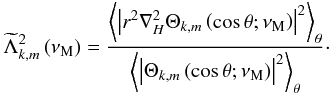 (85)
(85) and
and
 is the horizontal
spherical Laplacian.
is the horizontal
spherical Laplacian.
In the absence of rotation and of magnetic field (νM = 0),
we recover  . The
associated monochromatic vertical wave group velocity is given by
. The
associated monochromatic vertical wave group velocity is given by  (86)where
 is the monochromatic wave phase velocity in solar-type stars. Signs are due to the
direction of the excitation kinetic energy flux directed from the convective envelope to
the star’s center; in massive stars, signs are inverted. Finally, to determine
eigenfrequencies one has to follow strictly the same methodology as described in
Friedlander (1987a,b) and in Lee & Saio
(1989).
is the monochromatic wave phase velocity in solar-type stars. Signs are due to the
direction of the excitation kinetic energy flux directed from the convective envelope to
the star’s center; in massive stars, signs are inverted. Finally, to determine
eigenfrequencies one has to follow strictly the same methodology as described in
Friedlander (1987a,b) and in Lee & Saio
(1989).
4. The traditional approximation in the MHD case
4.1. Validity domain
The MHD TA can be applied in spherical shells where ![Mathematical equation: \begin{equation} {\mathcal D}\left(x;\nu_{\rm M}\right)=1-\nu_{\rm M}^{2}x^2>0\,\,\,\forall x\in\left[-1,1\right], \label{DMHDTA} \end{equation}](/articles/aa/full_html/2011/02/aa15571-10/aa15571-10-eq255.png) (87)thus as long
|νM| < 1 and
∀r and ∀θ ∈ [0,π] (cf. Fig. 6). In this regime, waves are elliptic and regular at all
latitudes. In the other case, where both
(87)thus as long
|νM| < 1 and
∀r and ∀θ ∈ [0,π] (cf. Fig. 6). In this regime, waves are elliptic and regular at all
latitudes. In the other case, where both  and
and  (|νM| ≥ 1 and ),
waves become hyperbolic and trapped in an equatorial belt (see Dintrans & Rieutord
2000, for example) where
θ ∈ [θc,π − θc],
with θc the critical colatitude
(|νM| ≥ 1 and ),
waves become hyperbolic and trapped in an equatorial belt (see Dintrans & Rieutord
2000, for example) where
θ ∈ [θc,π − θc],
with θc the critical colatitude  (88)where
 (cf. Fig. 7). Then, the adiabatic velocity field is
singular and the MHD TA cannot be applied (see Sect. 3.1, and references therein), because
the wave behaviour is possibly ruled by the dissipation in wave attractors (see for
example in the hydrodynamical case Dintrans et al. 1999; Dintrans & Rieutord 2000;
and Maas & Harlander 2007). This is a
strict generalization of the criteria derived in the hydrodynamical case for
gravito-inertial waves (Mathis et al. 2008; Mathis
2009).
(cf. Fig. 7). Then, the adiabatic velocity field is
singular and the MHD TA cannot be applied (see Sect. 3.1, and references therein), because
the wave behaviour is possibly ruled by the dissipation in wave attractors (see for
example in the hydrodynamical case Dintrans et al. 1999; Dintrans & Rieutord 2000;
and Maas & Harlander 2007). This is a
strict generalization of the criteria derived in the hydrodynamical case for
gravito-inertial waves (Mathis et al. 2008; Mathis
2009).
4.2. Wave classification
Under the MHD TA (as long as |νM| < 1), four types of magneto-gravito-inertial waves can be identified (see Townsend 2003; and Mathis et al. 2008, and references therein in the hydrodynamical case).
-
Class I waves. They are internal gravity waves, which exist in the non-rotating and in the non-magnetic cases, which are modified both by Coriolis acceleration and the Lorentz force. Their eigenvalue (Λk,m), hence their radial wave number,
 , are increased. Such
waves are also called magneto-Poincaré waves (see Zaqarashvili et al. 2009; Heng & Spitovsky 2009 and Sect. 2).
, are increased. Such
waves are also called magneto-Poincaré waves (see Zaqarashvili et al. 2009; Heng & Spitovsky 2009 and Sect. 2). -
Class II waves. They are purely retrograde waves (m > 0), which only exist in the case of νM high values. Their dynamics are driven by the conservation of the specific vorticity combined with the effects of curvature and by the Lorentz force. However, since |νM| ≥ 1 in this case, they cannot be treated using the MHD TA. In the hydrodynamical case, they are called “quasi-inertial” waves, which corresponds to the geophysical Rossby waves (see Provost et al. 1981). Such magneto-Rossby waves have recently been studied by Zaqarashvili et al. (2007), Zaqarashvili et al. (2009), and Heng & Spitovsky (2009) in the limit of a thin stratified layer.
-
Class III waves. These are mixed class I and class II waves, and m ≤ 0 waves exist in the absence of rotation and of magnetic field. Waves with m > 0 appear when νM = m + 1 with low eigenvalues, while their horizontal eigenfunctions are
 .
When they appear and have low eigenvalues, they behave mostly like class
II waves; m ≤ 0 and
m > 0 waves with high eigenvalues behave
rather like class I waves. Their eigenvalues are much lower than
those of class I waves. Thus, they have a smaller vertical wave
number. They may be identified with the geophysical Yanai waves (Yanai &
Maruyama 1966).
.
When they appear and have low eigenvalues, they behave mostly like class
II waves; m ≤ 0 and
m > 0 waves with high eigenvalues behave
rather like class I waves. Their eigenvalues are much lower than
those of class I waves. Thus, they have a smaller vertical wave
number. They may be identified with the geophysical Yanai waves (Yanai &
Maruyama 1966). -
Class IV waves. They are purely prograde waves (m < 0) whose characteristics change little with νM, since their displacement in the θ direction is very small. Their dynamics are driven by the conservation of the specific vorticity combined with the stratification effects and by the Lorentz force; their eigenvalues are lower than those of both class I and class III waves. Hence, their vertical wave number is smaller. In the hydrodynamical case, they may be identified with the geophysical Kelvin waves (Pedlosky 1998).
If we define a new index s by  (89)then Class
IV waves have s = −1, class III
waves s = 0, and class I waves have
s = 1,2,3,...
(89)then Class
IV waves have s = −1, class III
waves s = 0, and class I waves have
s = 1,2,3,...
5. Conclusion and perspectives
In this work, we examine of low-frequency internal wave behaviour in stellar radiation
zones, which are stable highly stratified rotating magnetic regions. Then, waves dynamics
are driven by the buoyancy force, the Coriolis acceleration, and the Lorentz force. Internal
waves thus become magneto-gravito-inertial waves that are equivalent to the MAC waves
(magnetic – Archimedean – Coriolis) which have been studied for the Earth’s core. In this
work in the stellar context, we studied the case of radiation zones with an axisymmetric
purely toroidal magnetic field, where both the angular velocity (Ωs) and the
Alfvén pulsation (ωA) are assumed to be uniform. This allowed to
extract the main properties of the system. First, we derived dynamical equations, following
Braginsky’s work and using stellar notations. Then, the MHD TA, which can be used only in
the strongly stratified case when
|νM| < 1 and
,
has been introduced and discussed. This allows to simplify the equations system and to
obtain in this case the wave-velocity field, the wave-magnetic field, and the total pressure
fluctuation as a function of the usual Hough functions and associated special latitudinal
and azimuthal functions used in the non-magnetic case for gravito-inertial waves in the
super-inertial strongly stratified regime
(νs < 1). Then, four classes of
magneto-gravito-inertial waves are indentified, while the asymptotic behaviour of such
low-frequency waves is discussed.
Once this study is achieved, two main works have to be engaged in the near future. The first one, is to examine the angular momentum transport by such waves in the “weak differential rotation case” (cf. Mathis et al. 2008), assuming a uniform Alfvén frequency to isolate the impact of an axisymmetric toroidal magnetic field as a function of its intensity (Paper II). Then, the more general case of general differential rotation and azimuthal magnetic field has to be studied, because it has been done in Mathis (2009) in the hydrodynamical case (Paper III). Moreover, the same methodology must be applied to axisymmetric poloidal magnetic fields. This will lead to a coherent picture of angular momentum wave-induced transport taking the impact of an axisymmetric fossil magnetic field into account.
The Alfvén speed associated to an axisymmetric toroidal magnetic field
( ) is given by
 .
Since
ωA = VA/s,
where s = rsinθ is the distance from
the symmetry axis, we get
.
Since
ωA = VA/s,
where s = rsinθ is the distance from
the symmetry axis, we get  . Here, we
choose a uniform ωA as a first step. The case of a general
realistic axisymmetric toroidal field
(ωA(r,θ))
will be treated in Paper III.
. Here, we
choose a uniform ωA as a first step. The case of a general
realistic axisymmetric toroidal field
(ωA(r,θ))
will be treated in Paper III.
The dynamical total pressure W is defined as W = Π/ρ.
Since ,
then  .
.
Here, we consider the case of solar-type stars for which the group velocity is negative
(cf. Eq. (86)). In the case of massive
stars, where it is positive, the phase function is ![Mathematical equation: \hbox{$\exp\left[{\rm i}\int_{\,r_{\rm c}}^{\,r}k_{V;k,m}\,{\rm d}r^{'}\right]$}](/articles/aa/full_html/2011/02/aa15571-10/aa15571-10-eq318.png) .
.
Acknowledgments
Authors thank Drs. A.-S. Brun, S. Talon, S. Turck-Chièze, and J.-P. Zahn for fruitful discussions during this work, which was supported in part by the Programme National de Physique Stellaire (CNRS/INSU), the CNES/GOLF grant at the Service d’Astrophysique (CEA – Saclay), and the CNRS Physique théorique et ses interfaces programme.
References
- Acheson, D. J. 1978, R. Soc. London Phil. Trans. Ser. A, 289, 459 [Google Scholar]
- Antia, H. M., Chitre, S. M., & Thompson, M. J. 2003, A&A, 399, 329 [NASA ADS] [CrossRef] [EDP Sciences] [Google Scholar]
- Barnes, G., MacGregor, K. B., & Charbonneau, P. 1998, ApJ, 498, L169 [NASA ADS] [CrossRef] [Google Scholar]
- Belkacem, K., Samadi, R., Goupil, M. J., et al. 2009, A&A, 494, 191 [NASA ADS] [CrossRef] [EDP Sciences] [Google Scholar]
- Bildsten, L., Ushomirsky, G., & Cutler, C. 1996, ApJ, 460, 827 [Google Scholar]
- Braginsky, S. I. 1967, Geomagnetism and Aeronomy, 7, 851 [NASA ADS] [Google Scholar]
- Braginsky, S. I., & Roberts, P. H. 1975, Proc. Royal Soc. London A, 347, 125 [NASA ADS] [CrossRef] [Google Scholar]
- Braithwaite, J. 2009, MNRAS, 397, 763 [NASA ADS] [CrossRef] [Google Scholar]
- Braithwaite, J., & Spruit, H. C. 2004, Nature, 431, 819 [NASA ADS] [CrossRef] [PubMed] [Google Scholar]
- Browning, M. K., Miesch, M. S., Brun, A. S., & Toomre, J. 2006, ApJ, 648, L157 [Google Scholar]
- Brun, A.-S., & Zahn, J.-P. 2006, A&A, 457, 665 [NASA ADS] [CrossRef] [EDP Sciences] [Google Scholar]
- Charbonnel, C., & Talon, S. 2005, Science, 309, 2189 [NASA ADS] [CrossRef] [PubMed] [Google Scholar]
- Cowling, T. G. 1941, MNRAS, 101, 367 [NASA ADS] [Google Scholar]
- Denissenkov, P. A., Pinsonneault, M., & MacGregor, K. B. 2008, ApJ, 684, 757 [NASA ADS] [CrossRef] [Google Scholar]
- Dintrans, B., & Rieutord, M. 2000, A&A, 354, 86 [NASA ADS] [Google Scholar]
- Dintrans, B., Rieutord, M., & Valdettaro, L. 1999, J. Fluid Mech., 398, 271 [NASA ADS] [CrossRef] [Google Scholar]
- Dintrans, B., Brandenburg, A., Nordlund, Å, & Stein, R. F. 2005, A&A, 438, 365 [NASA ADS] [CrossRef] [EDP Sciences] [Google Scholar]
- Duez, V., & Mathis, S. 2010, A&A , 517, A58 [NASA ADS] [CrossRef] [EDP Sciences] [Google Scholar]
- Eckart, C. 1960, Hydrodynamics of Oceans and Atmospheres (Oxford: Pergamon Press) [Google Scholar]
- Friedlander, S. 1987a, Geophys. J. Royal Astron. Soc., 89, 637 [Google Scholar]
- Friedlander, S. 1987b, Geophys. Astrophys. Fluid Dyn., 39, 315 [NASA ADS] [CrossRef] [Google Scholar]
- Friedlander, S. 1989, Geophys. Astrophys. Fluid Dyn., 48, 53 [NASA ADS] [CrossRef] [Google Scholar]
- Friedlander, S., & Siegmann, W. L. 1982, Geophys. Astrophys. Fluid Dyn., 19, 267 [NASA ADS] [CrossRef] [Google Scholar]
- Fruman, M. D. 2009, J. Atmos. Sci., 66, 2937 [NASA ADS] [CrossRef] [Google Scholar]
- Garaud, P., & Guervilly, C. 2009, ApJ, 695, 799 [NASA ADS] [CrossRef] [Google Scholar]
- Gerkema, T., & Shrira, V. I. 2005, J. Fluid Mech., 529, 195 [NASA ADS] [CrossRef] [Google Scholar]
- Gerkema, T., Zimmerman, J. T. F., Mass, L. R. M., & Van Haren, H. 2008, Rev. Geophys., 46, CiteID RG2004 [Google Scholar]
- Gough, D. O., & McIntyre, M. E. 1998, Nature, 394, 755 [NASA ADS] [CrossRef] [Google Scholar]
- Heng, K., & Spitkovsky, A. 2009, ApJ, 703, 1819 [NASA ADS] [CrossRef] [Google Scholar]
- Hough, S. S. 1898, Philos. Trans. Royal Soc. London A, 191, 139 [Google Scholar]
- Kiraga, M., Jahn, K., Stepien, K., & Zahn, J.-P. 2003, Acta Astron., 53, 321 [NASA ADS] [Google Scholar]
- Kiraga, M., Stepien, K., & Jahn, K. 2005, Acta Astron., 55, 205 [NASA ADS] [Google Scholar]
- Kumar, P., Talon, S., & Zahn, J.-P. 1999, ApJ, 520, 859 [NASA ADS] [CrossRef] [Google Scholar]
- Landau, L. D., & Lifchitz, E. M. 1966, Theoretical Physics: Quantum Mechanics (Moscow: Mir) [Google Scholar]
- Laplace, P.-S. 1799, Mécanique céleste, Bureau des Longitudes, Paris [Google Scholar]
- Lee, U. 2005, MNRAS, 357, 97 [NASA ADS] [CrossRef] [Google Scholar]
- Lee, U. 2007, MNRAS, 374, 1015 [Google Scholar]
- Lee, U. 2010, MNRAS, 405, 1444 [NASA ADS] [Google Scholar]
- Lee, U., & Saio, H. 1987, MNRAS, 225, 643 [NASA ADS] [Google Scholar]
- Lee, U., & Saio, H. 1989, MNRAS, 237, 875 [NASA ADS] [Google Scholar]
- Lee, U., & Baraffe, I. 1995, A&A, 301, 419 [NASA ADS] [Google Scholar]
- Lee, U., & Saio, H. 1997, ApJ, 491, 839 [NASA ADS] [CrossRef] [Google Scholar]
- Lindzen, R. S., & Chapman, S. 1969, Space Sci. Rev., 10, 3 [NASA ADS] [CrossRef] [Google Scholar]
- Longuet-Higgins, M. S. 1968, Philos. Trans. Royal Soc. of London A, 262, 511 [Google Scholar]
- Maas, L., & Harlander, U. 2007, J. Fluid Mech., 570, 47 [NASA ADS] [CrossRef] [Google Scholar]
- Markey, P., & Tayler, R. J. 1973, MNRAS, 163, 77 [NASA ADS] [CrossRef] [Google Scholar]
- Markey, P., & Tayler, R. J. 1974, MNRAS, 168, 505 [NASA ADS] [CrossRef] [Google Scholar]
- Mathis, S. 2009, A&A, 506, 811 [NASA ADS] [CrossRef] [EDP Sciences] [Google Scholar]
- Mathis, S., Talon, S., Pantillon, F.-P., & Zahn, J.-P. 2008, Sol. Phys., 251, 101 [NASA ADS] [CrossRef] [Google Scholar]
- Meynet, G., & Maeder, A. 2000, A&A, 361, 101 [NASA ADS] [Google Scholar]
- Mestel, L., Tayler, R. J., & Moss, D. L. 1988, MNRAS, 231, 873 [NASA ADS] [CrossRef] [Google Scholar]
- Pantillon, F. P., Talon, S., & Charbonnel, C. 2007, A&A, 474, 155 [NASA ADS] [CrossRef] [EDP Sciences] [Google Scholar]
- Pedlosky, J. 1998, Geophysical fluid dynamics, 2nd edn. (Springer) [Google Scholar]
- Press, W. 1981, ApJ, 245, 286 [NASA ADS] [CrossRef] [Google Scholar]
- Provost, J., Berthomieu, G., & Rocca, G. 1981, A&A, 94, 126 [NASA ADS] [Google Scholar]
- Rogers, T. M., & Glatzmaier, G. A. 2005, MNRAS, 364, 1135 [NASA ADS] [CrossRef] [Google Scholar]
- Rogers, T. M., & Glatzmaier, G. A. 2006, ApJ, 653, 756 [NASA ADS] [CrossRef] [Google Scholar]
- Rogers, T. M., & MacGregor, K. B. 2010, MNRAS, 401, 191 [NASA ADS] [CrossRef] [Google Scholar]
- Schatzman, E. 1993a, A&A, 271, L29 [NASA ADS] [Google Scholar]
- Schatzman, E. 1993b, A&A, 279, 431 [NASA ADS] [Google Scholar]
- Schecter, D. A., Boyd, J. F., & Gilman, P. A. 2001, ApJ, 551, L185 [NASA ADS] [CrossRef] [Google Scholar]
- Stewartson, K., & Richard, J. 1969, J. Fluid Mech., 35, 759 [NASA ADS] [CrossRef] [Google Scholar]
- Stewartson, K., & Walton, I. C. 1976, Proc. Royal Soc. London A, 349, 141 [Google Scholar]
- Talon, S. 2008, EAS PS, 32, 81 [Google Scholar]
- Talon, S., & Charbonnel, C. 2005, A&A, 440, 981 [NASA ADS] [CrossRef] [EDP Sciences] [Google Scholar]
- Talon, S., Kumar, P., & Zahn, J.-P. 2002, ApJ, 574, L175 [NASA ADS] [CrossRef] [Google Scholar]
- Tayler, R. J. 1973, MNRAS, 161, 365 [NASA ADS] [CrossRef] [Google Scholar]
- Tayler, R. J. 1980, MNRAS, 191, 151 [NASA ADS] [Google Scholar]
- Townsend, R. H. D. 2003, MNRAS, 340, 1020 [NASA ADS] [CrossRef] [Google Scholar]
- Unno, W., Osaki, Y., Ando, H., Saio, H., & Shibahashi, H. 1989, Non-radial oscillations of stars, second edition (Tokyo: University of Tokyo Press) [Google Scholar]
- Wright, G. A. E. 1973, MNRAS, 162, 339 [NASA ADS] [CrossRef] [Google Scholar]
- Yanai, M., & Maruyama, T. 1966, J. Meteorol. Soc. Japan, 44, 291 [Google Scholar]
- Zahn, J.-P. 1970, A&A, 4, 452 [NASA ADS] [Google Scholar]
- Zahn, J.-P. 1975, A&A, 41, 329 [NASA ADS] [Google Scholar]
- Zahn, J.-P. 1992, A&A, 265, 115 [NASA ADS] [Google Scholar]
- Zahn, J.-P., Talon, S., & Matias, J. 1997, A&A, 322, 320 [NASA ADS] [Google Scholar]
- Zaqarashvili, T. V., Olivier, R., Ballester, J. L., & Shergelashvili, B. M. 2007, A&A, 470, 815 [NASA ADS] [CrossRef] [EDP Sciences] [Google Scholar]
- Zaqarashvili, T. V., Olivier, R., & Ballester, J. L. 2009, ApJ, 691, L41 [NASA ADS] [CrossRef] [Google Scholar]
Appendix A: Magneto-gravito-inertial waves dispersion relation
To establish the dispersion relation of magneto-gravito-inertial waves, we follow the
method proposed in Kumar et al. (1999). As in our
simplified model, we assume that the angular velocity is uniform (Ω = Ωs),
while the unperturbed magnetic field is here (and only here) assumed to also be uniform
(i.e.  ).
We consider the short-wavelength limit, where spatial and temporal dependence of all
perturbed quantities are taken as proportional to
exp[i(k·r + σt)].
Then, the linearized momentum equation (Eq. (2)) is given by
).
We consider the short-wavelength limit, where spatial and temporal dependence of all
perturbed quantities are taken as proportional to
exp[i(k·r + σt)].
Then, the linearized momentum equation (Eq. (2)) is given by 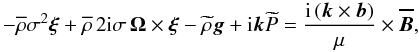 (A.1)where
 . Using the
energy transport equation in the adiabatic limit (Eq. (30)), this becomes
. Using the
energy transport equation in the adiabatic limit (Eq. (30)), this becomes
 (A.2)Substituting for
b using the linearized induction equation (Eq. (1)) in the case of a perfectly conducting fluid
and using the anelastic approximation that becomes in the short-wavelength
k·ξ = 0, we obtain
(A.2)Substituting for
b using the linearized induction equation (Eq. (1)) in the case of a perfectly conducting fluid
and using the anelastic approximation that becomes in the short-wavelength
k·ξ = 0, we obtain
![Mathematical equation: \appendix \setcounter{section}{1} \begin{eqnarray} &&-\overline\rho\sigma^2\vec\xi+\overline\rho\,2{\rm i}\sigma\,\vec\Omega\times\vec\xi+\overline\rho N^2 \xi_r\,{\widehat{\vec e}}_{r}+{\rm i}\vec k{\widetilde P} \nonumber\\ &&+\frac{\left(\vec{\overline B}\cdot\vec k\right)}{\mu}\left[\left(\vec{\overline B}\cdot\vec k\right)\vec\xi-\left(\vec{\overline B}\cdot\vec\xi\right)\vec k\right]=0 . \end{eqnarray}](/articles/aa/full_html/2011/02/aa15571-10/aa15571-10-eq290.png) (A.3)Taking
the vector cross product of the previous equation with k, we
get
(A.3)Taking
the vector cross product of the previous equation with k, we
get ![Mathematical equation: \appendix \setcounter{section}{1} \begin{equation} \left[\sigma^2\!-\!\left({\vec{\widehat{B}}}\cdot\vec k\right)^2V_A^2\right]\left(\vec k\times\vec\xi\right)-N^2\xi_r\left(\vec k\times{\widehat {\vec e}}_{r}\right)+2{\rm i}\sigma\left(\vec\Omega\cdot\vec k\right)\vec\xi\!=\!0 , \label{eqprev} \end{equation}](/articles/aa/full_html/2011/02/aa15571-10/aa15571-10-eq292.png) (A.4)where
(A.4)where
 is the Alfvén velocity and
  . Taking the
cross product of the previous equation with k allows
k × ξ as a function of
ξ. Substituting back in Eq. (A.4), we obtain
. Taking the
cross product of the previous equation with k allows
k × ξ as a function of
ξ. Substituting back in Eq. (A.4), we obtain
![Mathematical equation: \appendix \setcounter{section}{1} \begin{eqnarray} \lefteqn{\vec\xi\left\{-\frac{\left[\sigma^2-\left({\vec{\widehat{B}}}\cdot\vec k\right)^2V_{\rm A}^2\right]^2k^2}{2{\rm i}\sigma\left(\vec\Omega\cdot\vec k\right)}-2{\rm i}\sigma\left(\vec\Omega\cdot\vec k\right)\right\}}\nonumber\\ &+&\xi_{r}\left[N^2\left(\vec k\times{\widehat{\vec e}}_{r}\right)-\frac{N^2\left[\sigma^2-\left({\vec{\widehat{B}}}\cdot\vec k\right)^{2}V_{\rm A}^{2}\right]}{2 i \sigma \left(\vec\Omega\cdot\vec k\right)}\vec k\times\left(\vec k\times{\widehat{\vec e}}_{r}\right)\right]=0 .\nonumber\\ \end{eqnarray}](/articles/aa/full_html/2011/02/aa15571-10/aa15571-10-eq297.png) (A.5)Taking
the r-component of this equation gives the searched dispersion relation:
(A.5)Taking
the r-component of this equation gives the searched dispersion relation:
![Mathematical equation: \appendix \setcounter{section}{1} \begin{eqnarray} &&\left[\sigma^2-\left({\vec{\widehat{B}}}\cdot\vec{k}\right)^2V_{\rm A}^2\right]^2-\left(\vec N\times{\vec{\widehat{k}}}\right)^2\left[\sigma^2-\left({\vec{\widehat{B}}}\cdot\vec{k}\right)^2V_{\rm A}^2\right]\nonumber\\ &&-4\sigma^2\left(\vec\Omega\cdot\vec{\widehat{k}}\right)^2=0 , \label{LDR} \end{eqnarray}](/articles/aa/full_html/2011/02/aa15571-10/aa15571-10-eq299.png) (A.6)where
we have defined
(A.6)where
we have defined  and
and
 , which can be
inverted:
, which can be
inverted: ![Mathematical equation: \appendix \setcounter{section}{1} \begin{eqnarray} \sigma^2&=&\left({\vec{\widehat{B}}}\cdot\vec k\right)^2V_{\rm A}^{2}+ \frac{1}{2}\left\{\left(\vec N\times\vec{\widehat{k}}\right)^2+4\left(\vec\Omega\cdot{\vec{\widehat{k}}}\right)^2\right.\nonumber\\ &\pm &{\left.\!\!\sqrt{\left[\left(\vec N\!\times\!\vec{\widehat{k}}\right)^2\!+\!4\left(\vec\Omega\cdot{\vec{\widehat{k}}}\right)^2\right]^2\!+\!16\left(\vec{\widehat{B}}\cdot{\vec k}\right)^2V_{\rm A}^{2}\left(\vec\Omega\cdot{\vec{\widehat{k}}}\right)^2}\,\right\}} . \end{eqnarray}](/articles/aa/full_html/2011/02/aa15571-10/aa15571-10-eq302.png) (A.7)Two
branches can be isolated: the lower-frequency branch corresponds to the Alfvén waves
modified by the Coriolis acceleration, and the higher-frequency one is linked to the
magneto-gravito-inertial waves.
(A.7)Two
branches can be isolated: the lower-frequency branch corresponds to the Alfvén waves
modified by the Coriolis acceleration, and the higher-frequency one is linked to the
magneto-gravito-inertial waves.
Appendix B: The magneto-gravity waves case
In this short appendix, we simplify the general case treated here to unravel the magnetic
field impact on gravity waves. We thus do not take the Coriolis acceleration into account
(i.e.  ). Then,
νM becomes
). Then,
νM becomes
 (B.1)and the waves’ horizontal
structure is described by associated Hough functions. Moreover, the MHD TA can be applied
as long as |νM| < 1, which
corresponds to
(B.1)and the waves’ horizontal
structure is described by associated Hough functions. Moreover, the MHD TA can be applied
as long as |νM| < 1, which
corresponds to  (B.2)for propagative waves
for which
(B.2)for propagative waves
for which  .
.
All Figures
|
Fig. 1 The set-up to study internal wave dynamics in rotating and magnetic stellar radiation
zones. Angular velocity (Ωs) and Alfvén frequency
|
| In the text | |
|
Fig. 2 Wave types in a rotating and magnetic stellar radiation zone and associated frequencies (where fL is the Lamb’s frequency). Values for the Sun (⊙ ) at the bottom of the Tachocline are given in brackets. |
| In the text | |
|
Fig. 3 Inverse of the Rossby number (νs) as a function of
the frequency (σ/2π) for
axisymmetric waves |
| In the text | |
|
Fig. 4 Elsasser number (ΛE) as a function of the wave frequency in the
corotating frame |
| In the text | |
|
Fig. 5 Left: hough functions
Θk,m(cosθ;ν)
(Top) and associated latitudinal
|
| In the text | |
|
Fig. 6 Top: νM as a function of
νs and ΛE for non-axisymmetric retrograde
(m = 1) and prograde (m = −1) waves. The
surfaces such that |νM| = 1 are given by the thick
black lines and the iso-νM lines for
|νM| < 1 and
|νM| > 1 are given by
the red and the blue lines. The big external white region in the top-right corner
in each case corresponds to the |
| In the text | |
|
Fig. 7 Top: θc as a function of
νs and ΛE for non-axisymmetric retrograde
(m = 1) and prograde (m = −1) waves. As in
Fig. (6), the large white top-right corner
region corresponds to the |
| In the text | |
Current usage metrics show cumulative count of Article Views (full-text article views including HTML views, PDF and ePub downloads, according to the available data) and Abstracts Views on Vision4Press platform.
Data correspond to usage on the plateform after 2015. The current usage metrics is available 48-96 hours after online publication and is updated daily on week days.
Initial download of the metrics may take a while.