| Issue |
A&A
Volume 525, January 2011
|
|
|---|---|---|
| Article Number | A115 | |
| Number of page(s) | 11 | |
| Section | Extragalactic astronomy | |
| DOI | https://doi.org/10.1051/0004-6361/201015189 | |
| Published online | 06 December 2010 | |
One-zone models for spheroidal galaxies with a central supermassive black-hole
Self-regulated Bondi accretion
1
Dipartimento di AstronomiaUniversità di Bologna,
via Ranzani 1,
40127
Bologna,
Italy
e-mail: elisabeta.lusso2@unibo.it
2
INAF-Osservatorio Astronomico di Bologna,
via Ranzani 1,
40127
Bologna,
Italy
Received:
10
June
2010
Accepted:
24
September
2010
By means of a one-zone evolutionary model, we study the co-evolution of supermassive black holes and their host galaxies, as a function of the accretion radiative efficiency, dark matter content, and cosmological infall of gas. In particular, the radiation feedback is computed by using the self-regulated Bondi accretion. The models are characterized by strong oscillations when the galaxy is in the AGN state with a high accretion luminosity. We found that theseone-zone models are able to reproduce two important phases of galaxy evolution, namely an obscured-cold phase when the bulk of star formation and black hole accretion occur, and the following quiescent hot phase in which accretion remains highly sub-Eddington. A Compton-thick phase is also found in almost all models, associated with the cold phase. An exploration of the parameter space reveals that the closest agreement with the present-day Magorrian relation is obtained, independently of the dark matter halo mass, for galaxies with a low-mass seed black hole, and the accretion radiative efficiency ≃0.1.
Key words: galaxies: active / Galaxy: evolution / quasars: general
© ESO, 2010
1. Introduction
Elliptical galaxies invariably contain central supermassive black holes (SMBHs), and there exists a tight relationship between the characteristic stellar velocity dispersion σ (or stellar mass M∗) of the host system and the SMBH mass MBH (e.g., Magorrian et al. 1998; Ferrarese & Merritt 2000; Tremaine et al. 2002; Yu & Tremaine 2002). These relations clearly indicate a co-evolution of the SMBHs and their host spheroids. Several investigations have been dedicated to this subject, either by using hydrodynamical simulations (e.g., Ciotti & Ostriker 1997, 2001, 2007; Ciotti et al. 2009, 2010) or one-zone models (e.g., Sazonov et al. 2005,hereafter SOCS; Ballero et al. 2008, Matteucci 2008). In some work, the effect of galaxy merging has also been taken into account (e.g., Hopkins et al. 2005, 2006). The main advantage of hydrodynamical models is that complex physical phenomena effects (such as shock waves, jets, radiation transport, etc.) can be taken into account. However, the computational time of the simulations force us to search for faster methods that allow a more systematic exploration of the parameter space, which is prohibitive with hydrodynamical simulations. In this framework, hydro-simulations can be used to set the acceptable range for parameters to be adopted in toy models (e.g., the duty cycle value, see Sect. 2.1), while simpler models, such as that used here, are useful toidentify the most interesting cases that can be simulated in detail with hydrodynamical codes.
The general idea behind one-zone models is to work with “average” equations that capture some aspect of a more complicated situation. In practice, some of the equations are exact (such as for example the mass and energy balance equation). On the other hand, some of the physical variables are volume or mass averaged (e.g., the mean gas and temperature of the interstellar medium, respectively), or finally computed at some fiducial radius of the assumed gas distribution. From this point of view, the specific galaxy and dark matter halo profiles do not enter directly into the code, but are needed to obtain realistic mean values to be used in the equations.
A preliminary investigation of a physically based one-zone toy model has been done in SOCS, where it is shown that for a typical quasar spectral energy distribution (SED) the final MBH produced by feedback clearly reproduces the observed MBH-σ relation. The new models discussed here contain important improvements with respect to SOCS. First of all, the modelization of accretion onto SMBH. In this paper we examine how the effects of radiation pressure due to the Thomson electron scattering modify in a self-consistent way the spherical Bondi flow. Another improvement is the treatment of type Ia supernova rates and mass losses due to the evolution of the galactic stellar population, as we now adopt the Kroupa (2005) initial mass function (IMF) coupled with the evolutionary prescription of Maraston (2005). Finally, the dark matter halo is now described by a finite-mass Jaffe (1983) distribution instead of a singular isothermal sphere.
We focus on a scenario in which the masses of the central SMBH and the host galaxy grow in a dark matter halo, which is replenished by accretion of gas of cosmological origin. We follow star formation and we also consider the mass return from the evolving stellar populations. The combined effect of SNIa heating and radiative feedback, during episodes when the luminosity from the central SMBH approaches its Eddington limit, heats and drives much of the remaining gas out of the galaxy, limiting both future growth of the SMBH and future star formation to low levels. We do not consider the merging phenomenon, and we restrict ourselves to the evolution of an isolated galaxy: it is well known that significant AGN activity may also be present in isolated systems, because of the large amounts of gas produced by passively evolving stellar populations (e.g., Mathews 1983; Ciotti et al. 1991; Bregman & Parriott 2009; Kaviraj et al. 2010; Cisternas et al. 2010). More specifically, the one-zone models discussed in this paper are developed as an alternative approach to studying the “feedback modulated accretion flows” of Ciotti et al. (2009, 2010). There are two major differences between the present approach and hydro-simulations. The first, and most obvious, is the impossibility to resolve physical phenomena associated with specific length and timescales. The second is that we consider heating feedback only, while in the current version of the hydrodynamical code by Ciotti et al. (2009, 2010), both mechanical feedback, and radiation pressure are also considered. However, despite these shortcomings, with the present models we can attempt to simulate the process of galaxy formation, which is beyond the current possibilities of the hydro-simulations and at the same time we can explore the parameter space.
The evolutionary scenario that we consider here addresses several key observational findings. First, that giant ellipticals are old – they end their period of vigorous star formation early in cosmic time, since the radiative output from the central SMBHs limits (in cooperation with the energetic input due to star formation) the gas content to be at levels for which ongoing star formation is minimal. Secondly, gas-rich, actively star-forming galaxies at redshift z ~ 3, including Lyman break galaxies and bright submillimeter SCUBA galaxies, generally exhibit AGN activity (Steidel et al. 2002; Alexander et al. 2003; Alexander 2009; Lehmer et al. 2005; Donley et al. 2010), indicating that their central SMBHs continue to grow. This suggests that the formation of a spheroid probably closely preceeds a quasar shining phase, as verified by spectroscopic observations indicating that quasars occupy metal-enriched environments (e.g., Hamann & Ferland 1999; Schawinski et al. 2009; Wild et al. 2010). The redshift evolution of the quasar emissivity and the star formation history of spheroids is thus expected to have evolved roughly in parallel since z ~ 3, which is also consistent with observations (e.g., Haiman et al. 2004; Heckman et al. 2004). Among the most important observational predictions of the model is the length of the so-called “obscured accretion phase” (e.g., Comastri 2004). This phase is defined as the period of time when a high column density is associated with a high accretion rate onto the central SMBH. We also study the relation between the duration of the obscured phase and the corresponding “cold phase” (defined by a low mass-weighted gas temperature), and how they depend on the adopted parameters. Finally, in a large set of models we explore how the final SMBH mass is related to the final stellar mass, as a function of the dark matter halo mass, the amount of cosmological infall and the accretion rate of the gas, the SMBH accretion radiative efficiency, and finally the initial SMBH mass. We find that the models are in close agreement with the observed Magorrian relation when we assume high efficiencies (ϵ ~ 0.1) and relatively low initial SMBH masses (MBH ≲ 106 M⊙).
This paper is organized as follows. In Sect. 2, we present the physics adopted in the simulations, with special emphasis on the differences from and improvements on SOCS. Section 3 is devoted to the description of the adopted self-regulated accretion model, while in Sect. 4 we present our findings. The main results are summarized and discussed in Sect. 5, while several useful interpolating functions that we use to compute the stellar mass losses and the SNe Ia rate are presented in the Appendix.
2. The model
The galaxy model and the input physics adopted for the simulations have been improved with respect to SOCS, in particular the treatment of SNIa heating, the mass return rate from evolving stars, and the accretion onto the central SMBH. Several aspects of this model were described in SOCS and Ciotti & Ostriker (2007), and we present here only the relevant modifications.
2.1. The unchanged physics
For completeness, we briefly summarize the aspects of the input physics that remain unchanged with respect to SOCS. The differential equation for the gas mass balance is  (1)The first source term on the right-hand side (r.h.s.) describes the cosmological infall in a pre-existing (and time-independent) dark matter halo
  (2)where Minf is the total gas mass accreted during the simulation (but in general not equal to the final stellar galaxy mass M∗), and τinf is the characteristic infall timescale. A more appropriate description of the cosmological gas infall could be obtained by multiplying the r.h.s. of Eq. (2) by a factor t/τinf (e.g., Johansson et al. 2009), so that the total infalling mass is unaffected, while the infall starts in a more gentle way. For completeness, we performed some simulation with this different description, and we found (as expected) that for reasonable values of τinf the results are not much affected. Therefore, for consistency with SOCS we retain Eq. (2). The second source term is the net star-formation rate
  (3)where
  (4)is the instantaneous star-formation rate, and
  is the mass return by the evolving stellar population (Appendix A.1); following SOCS, in the simulations α∗ is fixed to be 0.3. The characteristic star-formation timescale τ∗ is defined as
  (5)where the dynamical timescale τdyn is given by Eq. (18), and the mean gas cooling time τcool is estimated to be
  (6)In the equation above, ĖC is the fiducial cooling rate given by
  (7)where
  is the instantaneous mean gas density (see Sect. 2.3),
  (8)is the cooling function (Mathews & Bregman 1978; see also Ciotti & Ostriker 2001), and X = 0.7 is the hydrogen mass abundance (for simplicity we assume complete ionization). In agreement with Eqs. (6) and (7), the mean gas internal energy is
  (9)where μ = (0.25 + 1.5X + 0.25Y)-1 ≃ 0.62 is the mean atomic weight. It follows that
  (10)where Mg is the instantaneous value of the total gas mass and rg is the gas distribution scale radius (Sect. 2.3). The third source term is the total accretion rate onto the SMBH
  (11)The first term describes gaseous accretion (Sect. 3), whereas the second term represents the contribution by the coalescence of stellar remnants of massive stars, as discussed in SOCS. The numerical coefficient fEdd ≈ 10-2−10-3 needs to be implemented in the one-zone code (which by definition is unable to model the different spatial scales of the problem) to represent the observed time variation of quasars. In practice, fEdd represents the “duty-cycle”, and its value is constrained by both observations (e.g. Yu & Tremaine 2002; Haiman et al. 2004) and simulations (Ciotti & Ostriker 2007; Ciotti et al. 2009, 2010). When the thermal energy of the interstellar medium (ISM) of the galaxy is high enough, the gas is able to escape from the dark matter potential well, at a fiducial escape rate computed as
  (12)The parameter ηesc is of the order of unity, while the expression for Tvir is given in the next section. Finally, the escape characteristic timescale is
  (13)where cs is the speed of sound and rg is the scale length of the gas distribution (Sect. 2.3). Energy input into the ISM is provided by the thermalization of supernova ejecta (both SNII and SNIa). The treatment of SNII is the same as in SOCS, and the new numerical treatment of SNIa is described in Appendix A.2. Additional contributions to the ISM energetics come from the thermalization of red giant winds and radiative feedback due to accretion onto the SMBH. As in SOCS, we adopt the average quasar SED obtained from the cosmic background radiation field supplemented by information from individual objects. We recall that the UV and high energy radiation from a typical quasar can photoionize and heat a low density gas up to an equilibrium Compton temperature (TC ≈ 2 × 10⁷ K) that exceeds the virial temperatures of giant ellipticals. Following SOCS, we also consider adiabatic cooling in the case of gas escaping and heating/cooling due to inflow/outflowing galactic gas. The gas temperature is therefore determined at each time-step by integrating the equation of the internal energy per unit volume
  (14)where ĖH,SN is the energy due to SNIa and SNII, ĖH,w describes the thermalization of red giant winds, ĖH,AGN is the AGN heating, Ėad is the adiabatic cooling in the case of galactic winds, and λ is a dimensionless parameter (
 ). Finally, we force the gas to remain above 104 K.
2.2. The dark matter halo
For simplicity, the dark matter (DM) halo in our model is the only contributor to the gravity of the galaxy. In addition, the gas and the stellar density distributions in the simulations are assumed to be proportional to the local (unevolving) DM density distribution, modeled as a Jaffe (1983) profile (Sect. 2.3)  (15)For a DM halo total mass Mh, the scale length rh is fixed following Lanzoni et al. (2004). In that paper, 13 massive DM halos obtained from high-resolution cosmological N-body simulations were carefully analyzed. In particular, for each halo the “overdensity radius” rΔ (sometimes called virial radius) was determined, and it was shown that rΔ does not differ significantly from the true virial radius rvir of the system (with a scatter ≲ 20%). Averaging over the 13 clusters reported in Table 2 in Lanzoni et al. (2004), we found that
  (16)where Mh is in 109 M⊙ and rΔ is in kpc units. For the Jaffe profile rvir = 2rh, and from Eq. (16) we can link the scale-length rh to Mh by assuming rvir = rΔ. We finally recall that the virial (3D) velocity dispersion associated with Eq. (15), is given by
  (17)The halo mean circular velocity is estimated as
  , and the dynamical time required in Eq. (5) is therefore given by
  (18)
(18)
2.3. The galaxy model
One of the new aspects of the model evolution investigated in this paper is the time extent of the Compton thin and Compton-thick phases, as defined at the end of this section. In SOCS, the adopted gas density distribution was a singular isothermal sphere and the major drawback of this choice for the evaluation of average quantities is the divergence of the total mass. For this reason, we now use the more realistic Jaffe density profile, i.e., we assume that at each time the gas density distribution is  (19)where rg is the gas scale radius and Mg is the instantaneous value of the total gas mass, obtained by integrating Eq. (1). For simplicity, rg = rh during the whole simulation. However, it is possible to generalize the present approach and consider a time-dependent rg.
The mean gas density, which is needed in Eqs. (7) and (9), is evaluated to be the instantaneous mean value within the half-mass radius rg (20)while the virial gas temperature Tvir is obtained from the hydrostatic equilibrium and the Jeans equations solved in the gravitational potential of the DM halo neglecting the self-gravity of the gas. Simple algebra then shows that
  (21)To quantify the relative importance of the optically thin and thick phases, the code computes the gas column density as
  (22)where MPg(R) is the projected gas mass enclosed in a circle of radius R, and the factor of 2 at the denominator takes into account that only one side of the gas column actually obscures the center. Therefore, the fiducial column density depends not only on the total gas mass, but also on the aperture radius adopted. To simulate observational work (e.g. Risaliti et al. 1999), we decided to define R to be one hundredth of the effective radius Re1, i.e., in Eq. (22) R ≅ 0.0074rg . From Eq. (A.17)
  (23)and rg is fixed during the simulation, ⟨ NH ⟩ depends only on Mg. We refer to the “thick” phase if ⟨ NH ⟩ ≥ 1024 cm-2, while galaxies with column density ⟨ NH ⟩ ≥ 1022 cm-2 are considered obscured.
2.4. The code
The simulations are performed by numerical integration of the previous evolutionary differential equations using a forward Euler scheme. The numerical code is based on the code developed in SOCS. The time step is defined as the minimum among the characteristic times associated with the different physical processes  (24)where the different subscripts indicate the specific aspect of the physics involved and, in general, for a quantity Xi, ti ≡ Xi/ | Ẋi | . The dimensionless coefficient B ≤ 1 is used to improve the code accuracy. We performed several test simulations and we found that B ≅ 0.1 leads to rapid convergence and excellent agreement with results obtained in SOCS, when used with their model galaxies and input physics.
3. Self-regulated Bondi accretion
As often assumed in the literature, the SMBH accretion rate is determined as the minimum between the Bondi accretion rate ṀB and Eddington limit ṀEdd (25)In the previous formula, the Eddington accretion rate is
  (26)where 0.001 ≲ ϵ ≲ 0.1 is the accretion efficiency, and
  (27)is the Eddington luminosity and σT is the Thomson cross-section. The classical Bondi accretion rate is
  (28)where ρ∞ and cs,∞ are the gas density and the speed of sound at infinity, respectively, and λc is a dimensionless coefficient of the order of unity (e.g., Bondi 1952; Krolik 1999). In Eq (28), radiative effects are not taken into account, so that in Eq. (25) there is a sharp transition between the pure hydrodynamical and radiation-dominated regimes. Fortunately, in the optical thin regime dominated by electron scattering, it is possible to extend the classical Bondi accretion solution and take into account the radiation pressure effects, so that the transition between Bondi-limited and Eddington-limited accretion can be described in a more consistent way. After solving this problem, we discovered that is had already been fully described by Taam et al. (1991) and Fukue (2001), and here we just summarize the main features of the modified accretion model. The result is obtained basically, by noting that in the optically thin regime the radiation pressure scales as 1/r2, thus reducing the effective gravitational force at each radius by the same amount. By imposing self-consistentcy, i.e. by requiring that the effective accretion rate
  is determined by the effective gravity, one finally obtains the following expression for the modified coefficient
  (29)Therefore, the self-consistent Bondi accretion rate satisfies the equation
 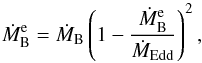 (30)that can be solved for . After discarding the unphysical solution, we have
 ![\begin{equation} \label{DMbhacc} \dotm\equiv\frac{\dotM}{\DMedd}=\frac{1}{2}\left[2+r-\sqrt{4r+r^2} \right],\quad r\equiv\frac{\DMedd}{\DMbon}\cdot \end{equation}](/articles/aa/full_html/2011/01/aa15189-10/aa15189-10-eq99.png) (31)For r → 0 (high accretion rates) ṁ → 1, so that tends to the Eddington accretion, while for r → ∞ (low accretion rates) ṁ → 0. The full solution is indicated in Fig. 1 by the heavy solid line: we note how Eq. (25) overestimates accretion onto SMBH in the range
(31)For r → 0 (high accretion rates) ṁ → 1, so that tends to the Eddington accretion, while for r → ∞ (low accretion rates) ṁ → 0. The full solution is indicated in Fig. 1 by the heavy solid line: we note how Eq. (25) overestimates accretion onto SMBH in the range  .
.
 |
Fig. 1 The self-regulated Bondi accretion rate |
4. Results
In the following sections, we present the main properties of a set of simulations, focusing on three important issues and comparing the new results with those in SOCS. However, before discussing the whole set of the new models, in the next section we present in detail the evolution of a representative model and three of its possible variants.
4.1. The evolution of the reference model and some of its variants
Figure 2 shows the time evolution of important quantities of our galaxy reference model (RM). This model is characterized by a DM halo of total mass Mh = 4 × 10¹¹ M⊙, which corresponds to a halo scale length rh = 11.86 kpc and Re = 8.83 kpc, a fiducial circular velocity calculated according to Eq. (17) of ~270 km s-1, and a characteristic infall time 2 Gyr. The assumed total mass of the cosmological gas infall is Minf = 1011 M⊙, corresponding to a dark-to-total mass ratio of 80% (provided that all the infalling gas forms stars). Other simulation parameters are α∗ = 0.3, βBH, ∗ = 1.5 × 10⁻⁴, ϵ = 0.1, ηSN = 0.85, ηesc = 2, and a stellar mass-to-light ratio of 5 (see Eq. (A.11)). As in SOCS, the initial SMBH mass is 108 M⊙; the duty circle, fEdd, is fixed at 0.005.
As can be seen from the comparison of Fig. 2 with Figs. 7 and 8 in SOCS, the global evolution of the new models is qualitatively very similar to those in SOCS. In particular, the time evolution of the model, from the beginning up to ~9 Gyr, is characterized by a cold phase (we assume that a cold phase corresponds to Tgas ≤ 105 K) of high density and low temperature. The gas density at the Bondi radius remains between 1 and 102 particles per cm3, while the mean gas density is ~10-1−10-2 particles per cm3. At the beginning of the cold phase, about 2.17 Gyr are spent in the Compton-thick phase (see Fig. 2d). The remaining part of the cold phase is obscured, while the accretion luminosity remains high, at LBH ≳ 1046 erg s-1. As soon as the mean gas density decreases (Fig. 2c green dotted line) the cooling becomes inefficient, the gas heating dominates, and the temperature increases to the virial temperature. The total duration of the cold phase is ~9 Gyr, which corresponds to a decrease in ⟨ NH ⟩ of about 2 orders of magnitude. The obscured phase lasts ~9.6 Gyr and the average column density is then around ⟨ NH ⟩ ~ 1020 cm-2. The durations of the cold and the obscured phases are very similar, and indeed, the two phases are related. Until the gas density is high, the gas can radiate efficiently the energy input due to the AGN, and its temperature remains below 105 K. Because of this large amount of cold gas, the star formation proceeds at high rates, until most of the gas is consumed. At this point, the radiative cooling of the gas becomes inefficient and the heating due to the AGN causes the gas temperature to increase. The combined effects of the gas consumption and the increase temperature stop the star formation. A specific feature of the cold phase can be seen in Fig. 2, where characteristic temperature oscillations are apparent. These oscillations, already presented and discussed in SOCS, are due to the combined effect of gas cooling and AGN feedback. They terminate when the gas density falls below some threshold determined by the cooling function and because less and less gas is produced by stars and accreted by the galaxy, while SNIa heating declines less strongly. When the density is high (at early times), the cooling time is instead, very short, and AGN heating is radiated efficiently. The two competitive effects produce the temperature (and density) oscillations. In the hydro-simulations, the spatial and temporal structures of these oscillations is quite complicated, as feedback and cooling act on several different spatial and temporal scales (from a month to 10 Myr). In the one-zone models, the oscillations are instead dependent on the “duty-cycle” parameter fEdd in Eq. (1), which is constrained by observational and theoretical studies (see Sect. 2.1).
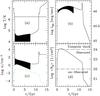 |
Fig. 2 The time evolution of relevant quantities of the RM. Panel (a): gas temperature; the virial temperature of the galaxy is the horizontal dashed line. Panel (b): bolometric accretion luminosity. Panel (c): gas density at the Bondi radius (black line) and the mean gas density (green dotted line). Panel (d): mean gas column density ⟨ NH ⟩ at aperture radius of 0.088 kpc. |
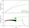 |
Fig. 3 The SMBH accretion history of the RM. Top panel: time evolution of the SMBH mass as computed according to SOCS (green line) and with the Bondi-modified accretion (black line). Bottom panel: SMBH accretion rate from SOCS (green line) and from our work (black line). The red solid line is the Eddington accretion rate for the SOCS model. |
Final properties of the RM and its variants at 15 Gyr.
To summarize, the observational properties of the RM would correspond to a system initially Compton-thick, that then switches to an obscured phase, and in the past 3.2 Gyr the galaxy is unobscured. The SMBH accretion history is shown in Fig. 3, where it is compared to that predicted by the SOCS formulation in a model otherwise identical to the RM. The major difference between the two models is in the final value of MBH: in particular, Eq. (25) would predict a present-day MBH a factor ~1.5 higher than that for modified accretion. This is because the accretion in SOCS remains for almost all of the galaxy life, at the Eddington limit, while in the new treatment the self-regulation maintains the accretion at lower rates.
Before presenting the results of a global exploration of the parameter space, we focus on a few obvious questions. For example, what happens if we keep all the model parameters fixed and reduce the radiative accretion efficiency? What happens if we increase or decrease the total mass of infalling gas? Or if we double the gas infalling time? Of course, these simple examples do not cover all the possible cases. However, these models will provide a guide as we investigate the parameter space. The relevant properties of the additional “reference” models are listed in Table 1.
The first variant of the RM model is model RM1 obtained by reducing the radiative accretion efficiency from ϵ = 0.1 to ϵ = 0.001. Overall, this reduced efficiency model passes through the same evolutionary phases as model RM: an initial Compton-thick phase, followed by an obscured phase, and finally a low-density unobscured phase. The initial cold high density phase is also very similar to that of RM in Fig. 2. The most important and expected difference is in the final mass of SMBH, which is higher by a factor of ≈3.5 than the RM. A reduction in the radiative efficiency also produces a slightly larger amount of escaped gas, because of the shorter cold phase. As a consequence, a larger amount of gas produced by the evolving stars is lost from the galaxy during the low-density, hot phase.
The effect of a reduction in Minf is explored in model RM2, while all the others parameters are the same as in RM. Qualitatively, the evolution is again very similar to that of RM in Fig. 2. The main difference is the absence of the initial Compton-thick phase because of the lower gas density. Both the final stellar mass and final SMBH mass are lower than in model RM, as can be seen from Table 1. Overall, model RM2 does not display remarkable or unexpectedproperties. The only noticeable aspect is that the escaped mass is higher than in model RM, but this is again due to the shorter cold phase.
A complementary model to RM2 is RM3, where we double the value of Minf while maintaining all the other parameters identical to those of model RM. The qualitative evolution is again similar to that of RM in Fig. 2, but, at variance with RM2, the Compton-thick phase is now present. Not surprisingly, the Compton-thick phase in model RM3 extends for a longer period (~5 Gyr) than in the other variants of RM (see Table 1), and its total mass of new stars is also the highest. However, the total mass that escapes is not as high as one would expect, the infall mass being a factor of 2 higher than in the RM yet the escaped mass being almost the same. The main reason for this behaviour is the very massive star formation, which is almost double that of RM. We note that model RM3 is the closest, in the RM family, to the galaxy models studied in the hydrodynamical simulations of Ciotti et al. (2009, 2010), as far as the final stellar mass and the final MBH are concerned.
We finally discuss model RM4, which is identical to model RM, but has twice as long an infall time. The main effects are the longest cold phase in RM family (see Table 1), and the absence of the initial Compton-thick phase. This latter characteristic is due to the time dilution of the infalling gas density, which prevents the possibility of reaching very high column density values. Overall, the final SMBH mass is not affected significantly by the extended infall phase, but its escaped gas masses is quite high because the total mass in new stars is (as expected) lower than in the RM model.
To summarize, these preliminary experiments have revealed that, at fixed dark matter halo, sensible variations in the input parameters do not produce remarkable different results. The relevant differences are found mainly in the amount of star formation and the different durations of the cold and obscured phases, while the final SMBH mass appears to be mainly affected by the value of the radiative efficiency ϵ.
Final properties of models with self-regulated Bondi accretion with an initial SMBH mass of 108 M⊙. All masses are in units of 109 M⊙.
Final properties of models with self-regulated Bondi accretion with an initial SMBH mass of 105 M⊙. All masses are in units of 109 M⊙.
4.2. Exploring the parameter space
We now present the general results (summarized in Tables 2 and 3) of our examination of the parameter space. The SMBH initial mass in the models in Table 2 is 108 M⊙, while in Table 3 it is 105 M⊙. From the astrophysical point of view, the first choice mimics a scenario in which the central SMBHs are already quite massive at the epoch of galaxy formation, while in the second case the main growth occurs with galaxy formation. Each of the 5 main families of models (M1, ..., M5) consists of galaxy models characterized by the same dark halo mass, Mh, ranging from 1010 M⊙ (the M1 family) up to 1012 M⊙ (the M5 family). In each family, we have investigated 6 models with different values of infalling gas-to-dark matter ratio α = Minf/Mh, and finally different radiative efficiencies ϵ in the self-regulated Bondi accretion. In practice, in each family we explore the effects of different total infalling gas mass and different efficiencies (spanning the commonly accepted range of values) at fixed Mh.
Almost independently of Mh and the initial value of MBH, we can recognize some general trends. For example in each group of 3 models characterized by identical parameters but decreasing ϵ, it is apparent how the total amount of stars formed decreases at decreasing ϵ, while the final MBH increases. In the total mass budget of the galaxy, an important quantity is the total mass of gas ejected, Mesc. As expected, we find that massive galaxies, with larger infall gas masses also eject more mass. However, in all cases, the escaped gas mass is much lower than the final stellar mass, i.e., ~10% of it.
Finally, higher final gas masses are obtained, at fixed Mh, for higher Minf and lower efficiencies, because of the less effective feedback. We note however that the product of ϵ and the mass accreted by the SMBH decreases with decreasing ϵ, i.e., even though the accreted mass is higher, the integrated energy output is lower, and so is the feedback effect2.
A qualitative illustration of the effect of the reduction in ϵ on the SMBH accretion history is shown in Fig. 4. When the efficiency decreases, the final mass of the SMBH increases and, we indicate by the green line, the corresponding evolution of identical models but with the SOCS treatment, i.e., where the accretion is determined by the minimum of ṀB and ṀEdd. As expected, the differences in MBH reduce with decreasing ϵ, because the Eddington accretion regime in the SOCS models (when the major differences from the Bondi-modified case are established), becomes less and less important, and approches ṀB.
All models have a transition phase from obscured to unobscured. The Compton-thick phase is present in almost all models that have a cold phase (18 of 30 simulations); however, in the less massive set of models (M1) the Compton-thick phase is absent. This is consistent with the scenario in which the majority of the most massive black holes spend a significant amount of time growing in an earlier obscured phase (see Kelly et al. 2010; Treister et al. 2010).
Finally, the mean SMBH-to-star ratio is not far from the value inferred from the present-day Magorrian et al. (1998) relation, though on the high mass side. This is not surprising, because of our use of a one-zone model. In any case, we emphasize that the SMBH feedback in the models was able to remove (in combination with star formation and/or gas escape) most of the infalling gas (which, if accreted onto the central SMBH in a cooling-flow like solution, would lead to the final SMBH masses being ~2 orders of magnitude higher than the observed ones).
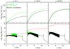 |
Fig. 4 Evolution of the SMBH mass and accretion rate computed according to Eqs. (25) (green line, SOCS) and (30) (black line) for a model with Minf = 1.25 × 10¹⁰ M⊙, Mh = 5 × 10¹⁰ M⊙, and initial SMBH mass of 108 M⊙. From left to right: ϵ = 0.1, ϵ = 0.01, and ϵ = 0.001. The red line represents the Eddington limit for the SOCS model. |
Independent of the particular characteristics of the single models, Fig. 5 clearly illustrates that the final SMBH masses, in models with a quite high initial MBH (Table 2), are higher than implied by the observed Magorrian relation. For this reason, we explored other families of models, in which the initial mass of the SMBH was reduced to 106 M⊙, 105 M⊙, and 103 M⊙. From Fig. 5, it is apparent how galaxy models with initial SMBH masses ≲ 106 M⊙ (circles) closely agree to within 1σ of the observed dispersion with observations, but only when the radiative efficiency is high, i.e. ϵ = 0.1. It is even more remarkable that the final SMBH mass is proportional to the final M∗, as all the models started with the same initial SMBH mass. This strongly indicates that co-evolution is the most plausible explanation of the proportionality between M∗ and MBH, in line with other observational evidence (e.g., see Haiman et al. 2004, and references therein).
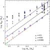 |
Fig. 5 Final SMBH mass versus final stellar mass for all the explored models. The solid line is the Marconi & Hunt (2003) best-fit of the Magorrian (1998) relation, and the two dashed lines represent the associated 1-σ deviation. Different colors indicate different initial masses of the MBH, i.e. 103 M⊙ (green), 105 M⊙ (red, models in Table 3), 106 M⊙ (blue), and 108 M⊙ (black, models in Table 2). Different symbols identify the adopted value for radiative efficiency: ϵ = 0.1 (circles), ϵ = 0.01 (triangles), and ϵ = 0.001 (squares). The black crosses are the hydrodynamical models in Table 1 of Ciotti et al. (2010). |
To compare our present findings with those of a complementary hydrodynamical approach, in Fig. 5 we plot the results of the high-resolution hydro-simulations developed by Ciotti et al. (2010, Table 1, Cols. 5 and 6) for a representative galaxy with stellar mass of ~3 × 10¹¹ M⊙. The final MBH are represented by crosses, and the different (luminosity weighted) radiative efficiencies are in the range 0.003 ≤ ϵ ≤ 0.133. We note that the crosses indicate almost all the hydrodynamical models that have been studied in detail so far, and this shows the importance of one-zone models as a complementary approach to exploring the parameter space. We also note thatthe final mass of the SMBHs, as computed in the hydrodynamical simulations, lead to an accurate reproduction of the Magorrian relation but the comparison with the one-zone models is delicate. In the hydrodynamical simulations (at variance with the one-zone models), the initial phases of galaxy formation are not simulated, and the focus is on the maintaining low SMBH masses in the presence of stellar mass losses that, if accreted onto the central SMBH as in an undisturbed cooling flow, would produce a final BH mass of about a factor of ~100 higher than the observed ones. For this reason, in the hydrodynamical models the galaxy is already assumed to have formed, and the initial mass of the SMBH is just slightly lower than the mass predicted by the Magorrian relation.
5. Conclusions
This paper is a natural extension of a previous paper by Sazonov et al. (2005). From a technical point of view, several aspects of the input physics have been improved. In particular, we have adopted a different description of the accretion rate, which now follows the self-consistent modified Bondi theory (Taam et al. 1991; Fukue 2001), instead of the minimum between the Eddington and the (classical) Bondi rate. Moreover, the SNIa rate is now computed using a high-precision multi-exponential approximation for the time-kernel in the convolution integral of the star formation rate, instead of the standard power-law. This avoids the need to store the entire star formation history and permits more rapid numerical simulations. The time-dependent mass return rate from the evolving stellar population is now computed using the Kroupa (2005) initial mass function and the mass return rate as a function of the stellar mass given by Maraston (2005), instead of the Ciotti et al. (1991) formulae. For the stellar mass-return rate, we also numerically implemented a multi-exponential fit. Finally, the dark-matter potential well (and the galaxy stellar distribution) are now described as Jaffe (1983) models.
From the astrophysical point of view, in addition to the standard outputs considered in SOCS (e.g. final SMBH mass, final stellar mass, etc), we now also focus on the duration of the “cold phase”, of the “obscured phase”, and the “Compton thick phase” as fiducially computed using the gas temperature and the column density of cold gas. The main parameters adopted to fix a model are the dark-matter halo mass (distributed to reproduce cosmological expectations), the amount of gas deemed to flow onto the dark matter halo, and finally the radiative accretion efficiency. As a separate parameter, we also consider the initial mass of the central SMBH. After some preliminary model exploration and verifying that the new treatment, when applied to the SOCS galaxy model reproduces the previous results, we performed a significant exploration of the parameter space.
Our main results can be summarized as follows:
-
1.
Almost independently of the dark matter halo mass and theradiative efficiency, the computed galaxy models have an initialphase that extends for some Gyrs, in which the gas temperature islow and the gas density is high. These galaxies would be definedobscured quasars, were we to measure their gas column densitywithin an aperture radius of the order of Re/100.
-
2.
At late times, all the SMBHs are found to be in a low accretion state without much feedback, and the ISM is overall optically thin. The galactic ISM is at about the virial temperature of the dark matter potential well and should be emitting in X-rays, as found for elliptical galaxies in the local universe.
-
3.
Interestingly, we have found that only a specific class of models, are found to agree with the observed Magorrian relation, i.e. only those with low initial SMBH masses (≲106 M⊙) and high radiative accretion efficiency, ϵ ~ 0.1. Higher initial SMBH masses, or lower radiative efficiencies lead to final SMBH masses that are too high. Therefore, this result implies that the seed SMBHs should be quite small, but that their mass accretion should occurmainly with high radiative efficiency, in agreement with observational findings.
-
4.
In addition, we have also showed how the self-regulated Bondi accretion recipe can be easily implemented in numerical codes, and how it leads to a lower SMBH mass accretion than the more common “on-off” Eddington regulation.
The second is that to reproduce the present-day Magorrian relation, the optimal combination of parameters is a quite low initial SMBH mass and a quite high radiative efficiency. We propose that this represents a useful constrain of semi-analytical investigations (also in the context of high-z galaxy merging). As a side-product of this work, we also anticipate that the presented multi-exponential fit for stellar evolution and SNIa heating will be useful in both hydrodynamical and semi-analytical works.
As a final comment, we point out a major improvement in the code. In a future study, we will relax the assumption of a fixed gas density distribution, imposing a time dependence of rg(t) as a function of the gas thermal content at that given time. We expect that this additional ingredient will cause the models to become more sensitive to the adopted parameters on the one hand by increasing the gas density during the cold phases (hence producing a stronger feedback by decreasing the value of the ionization parameter and increasing the mass accretion rate), and on the other hand by decreasing the gas density during the hot phase, so reducing further the Eddington ratios at late times. We naturally, also expect that both the star-formation and accretion histories, as well as the durations of the obscured and Compton-thick phases to be affected.
Acknowledgments
The anonymous referee is acknowledged for his/her comments that greatly improved the paper. We thank A. Comastri and J. P. Ostriker for useful discussions, and F. Marinacci for suggestions on the numerical code. The project is supported by ASI-INAF under grants I/023/05/00.
References
- Alexander, D. M., Bauer, F. E., Brandt, W. N., et al. 2003, AJ, 125, 383 [NASA ADS] [CrossRef] [Google Scholar]
- Alexander, D. M., 2009 Galaxy Evolution: Emerging Insights and Futur Challenges, ed. S. Jogee et al., ASP Conf. Ser., 419, 381 [Google Scholar]
- Ballero, S. K., Matteucci, F., Ciotti, L., Calura, F., & Padovani P., 2008, A&A, 478, 335 [NASA ADS] [CrossRef] [EDP Sciences] [Google Scholar]
- Bondi, H. 1952, MNRAS, 112, 195 [NASA ADS] [CrossRef] [MathSciNet] [Google Scholar]
- Bregman, J. N., & Parriott, J. R. 2009, ApJ, 699, 923 [NASA ADS] [CrossRef] [Google Scholar]
- Ciotti, L., D’Ercole, A., Pellegrini, S., & Renzini, A. 1991, ApJ, 376, 380 [NASA ADS] [CrossRef] [Google Scholar]
- Ciotti, L., & Ostriker, J. P. 1997, ApJ, 487, L105 [NASA ADS] [CrossRef] [Google Scholar]
- Ciotti, L., & Ostriker, J. P. 2001, ApJ, 551, 131 [NASA ADS] [CrossRef] [Google Scholar]
- Ciotti, L., & Ostriker, J. P. 2007, ApJ, 1038, 1056 [Google Scholar]
- Ciotti, L., Ostriker, J. P., & Proga, D. 2009, ApJ, 699, 89 [NASA ADS] [CrossRef] [Google Scholar]
- Ciotti, L., Ostriker, J. P., & Proga, D. 2010, ApJ, 717, 708 [NASA ADS] [CrossRef] [Google Scholar]
- Cisternas, M., Jahnke K., Inskip, K. J. et al. 2010, ApJ, accepted [arXiv:1009.3265] [Google Scholar]
- Comastri, A. 2004, in Supermassive Black Holes in the Distant Universe, Astrophys. Space Sci. Lib., 308, 245 [Google Scholar]
- Donley, J. L., Rieke, G. H., Alexander, D. M., Egami, E., & Pérez-González, P. G. 2010, ApJ, 719, 1393 [NASA ADS] [CrossRef] [Google Scholar]
- Ferrarese, L., & Merritt, D. 2000, ApJ, 539, L9 [NASA ADS] [CrossRef] [Google Scholar]
- Fukue, J. 2001, PASJ, 687, 692 [Google Scholar]
- Haiman, Z., Ciotti, L., & Ostriker, J. P. 2004, ApJ, 606, 763 [NASA ADS] [CrossRef] [Google Scholar]
- Hamann, F., & Ferland, G. 1999, ARA&A, 37, 487 [NASA ADS] [CrossRef] [Google Scholar]
- Heckman, T. M., Kauffmann, G., Brinchmann, J., et al. 2004, ApJ, 613, 109 [NASA ADS] [CrossRef] [Google Scholar]
- Hopkins, P. F., Hernquist, L., Cox, T. J. 2005, ApJ, 630, 705 [NASA ADS] [CrossRef] [Google Scholar]
- Hopkins, P. F., Hernquist, L., Cox, T. J. 2006, ApJS, 163, 1 [Google Scholar]
- Jaffe, W. 1983, MNRAS, 202, 995 [NASA ADS] [Google Scholar]
- Johansson, P. H., Naab, T., & Ostriker, J. P. 2009, ApJ, 697, L38 [NASA ADS] [CrossRef] [Google Scholar]
- Kaviraj, S., Schawinski, K., Silk, J., & Shabala, S. S. 2010, [arXiv:1008.1583] [Google Scholar]
- Kelly, B. C., Vestergaard, M., Fan, X. A. 2010, ApJ, 719, 1315 [NASA ADS] [CrossRef] [Google Scholar]
- Krolik, J. H. 1999, Active galactic nuclei: from the central black hole to the galactic environment (Princeton University Press) [Google Scholar]
- Kroupa, P. 2001, MNRAS, 231, 246 [Google Scholar]
- Lanzoni, B., Ciotti, L., Cappi, A., Tormen, G., & Zamorani, G. 2004, ApJ, 640, 649 [Google Scholar]
- Lehmer, B. D., Brandt, W. N., Alexander, D. M., et al. 2005, AJ, 129, 1 [NASA ADS] [CrossRef] [Google Scholar]
- Magorrian, J., Tremaine, S., Richstone, D. 1998, AJ, 115, 2285 [NASA ADS] [CrossRef] [Google Scholar]
- Maraston, C. 2005, MNRAS, 799, 825 [Google Scholar]
- Marconi, A., & Hunt, L. K. 2003, ApJ, 589, L21 [NASA ADS] [CrossRef] [Google Scholar]
- Mathews, W. G. 1983, ApJ, 272, 390 [Google Scholar]
- Mathews, W. G., & Bregman, J. N. 1978, ApJ, 224, 308 [NASA ADS] [CrossRef] [Google Scholar]
- Matteucci, F. 2008, [arXiv:0804.1492] [Google Scholar]
- Risaliti, G., Maiolino, R., & Salvati, M. 1999, ApJ, 522, 157 [NASA ADS] [CrossRef] [Google Scholar]
- Sazonov, S.Yu., Ostriker, J. P., Ciotti, L., & Sunyaev, R. A.2005, MNRAS, 358, 168 (SOCS) [NASA ADS] [CrossRef] [Google Scholar]
- Schawinski, K., Lintott, C. J., Thomas, D., et al. 2009, ApJ, 690, 1672 [NASA ADS] [CrossRef] [Google Scholar]
- Steidel, C. C., Hunt, M. P., Shapley, A. E., et al. 2002, ApJ, 576, 653 [NASA ADS] [CrossRef] [Google Scholar]
- Taam, R. E., & Fu, A. 1991, ApJ, 696, 707 [Google Scholar]
- Treister, E., Urry, C. M., Schawinski, K., Cardamone, C. N., & Sanders, D. B. 2010, ApJ, 722, L238 [NASA ADS] [CrossRef] [Google Scholar]
- Tremaine, S., Gebhardt, K., Bender, R., et al., 2002, ApJ, 574, 740 [NASA ADS] [CrossRef] [Google Scholar]
- Yu, Q., & Tremaine, S. 2002, ApJ, 335, 965 [Google Scholar]
- Wild, V., Heckman, T., & Charlot, S. 2010, MNRAS, 405, 933 [NASA ADS] [Google Scholar]
Appendix A: Interpolating functions for stellar evolution
Multi-exponential expansion parameters (in Gyr) for stellar mass losses and SNIa rate. Note that for SNIa the coefficients ai are dimensionless.
A.1. Stellar mass losses
The general expression for the stellar mass-return rate from an evolving stellar
population is  (A.1)where
 is the instantaneous star-formation rate and
W∗(t − t′) is the
normalized stellar death rate for a stellar population of age
t − t′. For an initial mass function (IMF) of
unitary total mass and age t,
is the instantaneous star-formation rate and
W∗(t − t′) is the
normalized stellar death rate for a stellar population of age
t − t′. For an initial mass function (IMF) of
unitary total mass and age t, ![\appendix \setcounter{section}{1} \begin{equation} \label{Wdef} \W(t)={\rm IMF}[\Mto]\vert\DMto\vert \Delta M^{\rm w}[\Mto], \end{equation}](/articles/aa/full_html/2011/01/aa15189-10/aa15189-10-eq261.png) (A.2)where
MTO(t) is the mass of stars entering the
turn-off at time t, and ΔMw their mass
loss. Following Ciotti & Ostriker (2007),
we assume that
(A.2)where
MTO(t) is the mass of stars entering the
turn-off at time t, and ΔMw their mass
loss. Following Ciotti & Ostriker (2007),
we assume that  (A.3)In
our models, we adopt a Kroupa (2001) IMF, with a minimum mass of 0.08
M⊙ and a maximum mass of 100
M⊙, while
ṀTO(t) is taken from Maraston (2005)
(A.3)In
our models, we adopt a Kroupa (2001) IMF, with a minimum mass of 0.08
M⊙ and a maximum mass of 100
M⊙, while
ṀTO(t) is taken from Maraston (2005)
 (A.4)In
the formula above, t is in yrs and MTO in
solar masses. The main computational problem posed by the evaluation of the integral in
Eq. (A.1) is that, in principle, the
entire history of
(A.4)In
the formula above, t is in yrs and MTO in
solar masses. The main computational problem posed by the evaluation of the integral in
Eq. (A.1) is that, in principle, the
entire history of  must be stored, which
requires a prohibitively large amount of memory and computational time. In the special
case of an exponential time dependence of W∗, this problem
can be fortunately avoided, as shown in Ciotti &
Ostriker (2001, 2007). In the present
case, W∗ is not an exponential function, being more similar
to a power law. However, we assume that a fit in terms of exponentials has been
obtained, i.e.
must be stored, which
requires a prohibitively large amount of memory and computational time. In the special
case of an exponential time dependence of W∗, this problem
can be fortunately avoided, as shown in Ciotti &
Ostriker (2001, 2007). In the present
case, W∗ is not an exponential function, being more similar
to a power law. However, we assume that a fit in terms of exponentials has been
obtained, i.e.  (A.5)where the
timescales ai and
bi are known. From the above equation
and Eq. (A.1), it follows that
(A.5)where the
timescales ai and
bi are known. From the above equation
and Eq. (A.1), it follows that
 (A.6)where
 (A.7)We divide the integral
into
(A.7)We divide the integral
into  (A.8)where
δt represents the last time-step. The evaluation of the first
integral can be done by using a simple trapezoidal rule and only the values of
at t and t − δt are required. The
second integral is transformed by adding and subtracting δt in the
exponential term, and simple algebra finally shows that
(A.8)where
δt represents the last time-step. The evaluation of the first
integral can be done by using a simple trapezoidal rule and only the values of
at t and t − δt are required. The
second integral is transformed by adding and subtracting δt in the
exponential term, and simple algebra finally shows that ![\appendix \setcounter{section}{1} \begin{equation} \label{dMwindfin} F_i(t)= \frac{\delt}{2} \left[\DMstarp(t) + {\rm e}^{-\frac{\delt}{b_i}}\DMstarp(t-\delt) \right] + {\rm e}^{-\frac{\delt}{b_i}}F_i(t-\delt). \end{equation}](/articles/aa/full_html/2011/01/aa15189-10/aa15189-10-eq279.png) (A.9)Therefore, the
introduction of the multi-exponential fit allow us to compute the instantaneous mass
return rate at time t just by storing the values of the
Fi functions at the previous time-step.
We performed a non-linear fit of the tabulated values of Eq. (A.2) (obtained with the exact formulae). We
found that an acceptable approximation over the entire Hubble time is obtained with the
coefficients in the first row of Table A.1 (with
a percentage error of at most of 10% and only at very late times, when the mass return
rate of a stellar population is negligible).
(A.9)Therefore, the
introduction of the multi-exponential fit allow us to compute the instantaneous mass
return rate at time t just by storing the values of the
Fi functions at the previous time-step.
We performed a non-linear fit of the tabulated values of Eq. (A.2) (obtained with the exact formulae). We
found that an acceptable approximation over the entire Hubble time is obtained with the
coefficients in the first row of Table A.1 (with
a percentage error of at most of 10% and only at very late times, when the mass return
rate of a stellar population is negligible).
A.2. SN Ia
In a given simple stellar population, the total (i.e. volume-integrated) energy release
by SNIa is  (A.10)where
ESN = 1051 erg is the fiducial energy released
by SNIa event and RSN is the SNIa rate. From Eqs. (11), (12)
in Ciotti & Ostriker (2007), the SNIa rate
for a stellar population of mass M∗ can be written as
(A.10)where
ESN = 1051 erg is the fiducial energy released
by SNIa event and RSN is the SNIa rate. From Eqs. (11), (12)
in Ciotti & Ostriker (2007), the SNIa rate
for a stellar population of mass M∗ can be written as
![\appendix \setcounter{section}{1} \begin{equation} \label{RSN} \RSN(t)=\frac{1.6 \times 10^{-13}}{\NBsun}\frac{M_*}{\Msun} \left(\frac{t}{t_{\rm H}}\right)^{-s} \;\;\;\qquad[\yrs^{-1}], \end{equation}](/articles/aa/full_html/2011/01/aa15189-10/aa15189-10-eq285.png) (A.11)where we adopt a
stellar mass-to-light ratio ΥB ⊙ = 5,
θSN = 1, h = 0.7,
tH = 13.7 Gyr, and s = 1.1. In our model
with a star formation rate of Ṁ∗, it follows that in each
time-step an amount Ṁ∗δt of stars is added
to the galaxy body. Therefore, the instantaneous total rate of SNIa explosion at time
t is
(A.11)where we adopt a
stellar mass-to-light ratio ΥB ⊙ = 5,
θSN = 1, h = 0.7,
tH = 13.7 Gyr, and s = 1.1. In our model
with a star formation rate of Ṁ∗, it follows that in each
time-step an amount Ṁ∗δt of stars is added
to the galaxy body. Therefore, the instantaneous total rate of SNIa explosion at time
t is  (A.12)We expanded the
dimensionless power-law kernel in the integral above again using a (dimensionless)
multi-exponential function, so that all the considerations in Sect. A.1 hold and in particular Eq. (A.9). The functions Fi
now contain new values of bi (in units of
Gyr-1). The parameters of the multi-exponential fit (with percentual errors
<3% over 13.7 Gyr) are listed in the second row of Table A.1. Therefore,
(A.12)We expanded the
dimensionless power-law kernel in the integral above again using a (dimensionless)
multi-exponential function, so that all the considerations in Sect. A.1 hold and in particular Eq. (A.9). The functions Fi
now contain new values of bi (in units of
Gyr-1). The parameters of the multi-exponential fit (with percentual errors
<3% over 13.7 Gyr) are listed in the second row of Table A.1. Therefore,
 (A.13)and
finally, the average SNIa heating per unit time and unit volume, needed in the gas
energy equation is
(A.13)and
finally, the average SNIa heating per unit time and unit volume, needed in the gas
energy equation is  (A.14)where again we use
half-mass values.
(A.14)where again we use
half-mass values.
A.3. Column density for the Jaffe model
In our model the gas density at each computation time is assumed to be proportional to
ρh and given by Eq. (19). The corresponding projected gas distribution is  (A.15)We
note that the projected density formally diverges for R → 0, so that,
to estimate a realistic value of the column density we need to compute a mean value of
the projected density within a fiducial aperture. The explicit formulae for
Σg(R), and the associated projected mass encircled with
R, MPg(R), are given in
Jaffe (1983). In particular, to estimate ⟨ NH ⟩ in
Eq. (22) we consider
MPg(R)
(A.15)We
note that the projected density formally diverges for R → 0, so that,
to estimate a realistic value of the column density we need to compute a mean value of
the projected density within a fiducial aperture. The explicit formulae for
Σg(R), and the associated projected mass encircled with
R, MPg(R), are given in
Jaffe (1983). In particular, to estimate ⟨ NH ⟩ in
Eq. (22) we consider
MPg(R)  (A.16)Integration
of Eq. (A.16) yields
(A.16)Integration
of Eq. (A.16) yields ![\appendix \setcounter{section}{1} \begin{equation} \label{Mprojsol} \begin{array}{l} \end{array} \frac{\MPg}{M_{\rm g}}=\Rtilde \left\{ \begin{array}{l} \displaystyle \frac{\pi}{2}-\frac{\Rtilde ~{\rm arcsech}\Rtilde}{\sqrt{1-\Rtilde^2}}, \; 0<\Rtilde<1; \\[3.5mm] \displaystyle \frac{\pi}{2}-\frac{\Rtilde ~{\rm arcsec}\Rtilde}{\sqrt{\Rtilde^2-1}}, \; \Rtilde>1; \\ \end{array}\right. \end{equation}](/articles/aa/full_html/2011/01/aa15189-10/aa15189-10-eq306.png) (A.17)where
(A.17)where
 and
MPg(rg) = (π/2−1)Mg.
and
MPg(rg) = (π/2−1)Mg.
All Tables
Final properties of models with self-regulated Bondi accretion with an initial SMBH mass of 108 M⊙. All masses are in units of 109 M⊙.
Final properties of models with self-regulated Bondi accretion with an initial SMBH mass of 105 M⊙. All masses are in units of 109 M⊙.
Multi-exponential expansion parameters (in Gyr) for stellar mass losses and SNIa rate. Note that for SNIa the coefficients ai are dimensionless.
All Figures
|
Fig. 1 The self-regulated Bondi accretion rate |
| In the text | |
|
Fig. 2 The time evolution of relevant quantities of the RM. Panel (a): gas temperature; the virial temperature of the galaxy is the horizontal dashed line. Panel (b): bolometric accretion luminosity. Panel (c): gas density at the Bondi radius (black line) and the mean gas density (green dotted line). Panel (d): mean gas column density ⟨ NH ⟩ at aperture radius of 0.088 kpc. |
| In the text | |
|
Fig. 3 The SMBH accretion history of the RM. Top panel: time evolution of the SMBH mass as computed according to SOCS (green line) and with the Bondi-modified accretion (black line). Bottom panel: SMBH accretion rate from SOCS (green line) and from our work (black line). The red solid line is the Eddington accretion rate for the SOCS model. |
| In the text | |
|
Fig. 4 Evolution of the SMBH mass and accretion rate computed according to Eqs. (25) (green line, SOCS) and (30) (black line) for a model with Minf = 1.25 × 10¹⁰ M⊙, Mh = 5 × 10¹⁰ M⊙, and initial SMBH mass of 108 M⊙. From left to right: ϵ = 0.1, ϵ = 0.01, and ϵ = 0.001. The red line represents the Eddington limit for the SOCS model. |
| In the text | |
|
Fig. 5 Final SMBH mass versus final stellar mass for all the explored models. The solid line is the Marconi & Hunt (2003) best-fit of the Magorrian (1998) relation, and the two dashed lines represent the associated 1-σ deviation. Different colors indicate different initial masses of the MBH, i.e. 103 M⊙ (green), 105 M⊙ (red, models in Table 3), 106 M⊙ (blue), and 108 M⊙ (black, models in Table 2). Different symbols identify the adopted value for radiative efficiency: ϵ = 0.1 (circles), ϵ = 0.01 (triangles), and ϵ = 0.001 (squares). The black crosses are the hydrodynamical models in Table 1 of Ciotti et al. (2010). |
| In the text | |
Current usage metrics show cumulative count of Article Views (full-text article views including HTML views, PDF and ePub downloads, according to the available data) and Abstracts Views on Vision4Press platform.
Data correspond to usage on the plateform after 2015. The current usage metrics is available 48-96 hours after online publication and is updated daily on week days.
Initial download of the metrics may take a while.