| Issue |
A&A
Volume 524, December 2010
|
|
|---|---|---|
| Article Number | A65 | |
| Number of page(s) | 22 | |
| Section | Astronomical instrumentation | |
| DOI | https://doi.org/10.1051/0004-6361/200913356 | |
| Published online | 24 November 2010 | |
Estimating the phase in groundbased interferometry: performance comparison between singlemode and multimode schemes
Laboratoire d’Astrophysique, Observatoire de Grenoble,
38041
Grenoble Cedex,
France
e-mail: This email address is being protected from spambots. You need JavaScript enabled to view it.
Received:
25
September
2009
Accepted:
6
September
2010
Abstract
Aims. We compare the performance of multi and singlemode interferometry for estimating the phase of the complex visibility.
Methods. We provide a theoretical description of the interferometric signal that enables us to derive the phase error with detector, photon, and atmospheric noises, for both multi and singlemode cases.
Results. We show that despite the loss of flux which occurs when the light is injected in the singlemode component (i.e. singlemode fibers, integrated optics), the spatial filtering properties of these singlemode devices often enable a better performance than multimode concepts. In the high-flux regime, which is speckle-noise dominated, singlemode interferometry is always more efficient, and its performance is significantly better when the correction provided by adaptive optics becomes poor, by a factor of 2 and more when the Strehl ratio is lower than 10%. In low-light level cases (detector noise regime), multimode interferometry reaches better performance, yet the gain never exceeds ~20%, which corresponds to the percentage of photon loss caused by the injection in the guides. Besides, we demonstrate that singlemode interferometry is also more robust to the turbulence for both fringe tracking and phase referencing, with the exception of narrow fields of view (≲ 1′′).
Conclusions. Our conclusion is therefore that from a theoretical point of view and contrarily to a widespread opinion, fringe trackers built with singlemode optics should be considered as a both practical and competitive solution.
Key words: instrumentation: interferometers / methods: analytical / techniques: interferometric
© ESO, 2010
1. Introduction
Performance of groundbased optical interferometers is severely limited by the atmospheric turbulent piston, which introduces a random optical path difference between the beams that are combined to produce fringes. These fringes are thus randomly moving on the detector, blurring the signal and preventing us from integrating on time longer than the coherence time of the atmosphere, typically a few tens of milliseconds in the infrared. As a consequence, the limiting-magnitude and ultimate precision of groundbased interferometers are dramatically reduced.
By estimating and compensating in real-time the interferometric phase – in other words by “locking” the fringes on the detector, fringe tracking and phase referencing devices are powerful instruments to circumvent this problem, allowing us to integrate the interferograms on much longer time frames. These instruments, which noticeably improve the sensitivity and the accuracy of interferometers, are undergoing major developments in recent few years, as the number of concepts that are currently studied for various interferometers (Le Bouquin et al. 2008; Sahlmann et al. 2008: VLTI; Berger et al. 2008: CHARA; Jurgenson et al. 2008: MROI) can attest.
In all the different concepts proposed, one key issue still in debate among the instrumental community is the relevance of using spatial filtering devices such as singlemode fibers or integrated optics to carry/combine the beams. It is often argued that spatial filtering is not suited for that type of instruments,
because only a fraction of the total flux is injected in the spatial filter component. This coupling efficiency, which is typically on the order of the Strehl ratio (Coudé du Foresto et al. 2000), can indeed be low with strong turbulence and/or poor adaptive optics (AO) correction. However, the case is not that simple. Singlemode filters only keep that part of the incoming flux which is related to the coherent part of the corrugated wavefront. In other words, singlemode devices only propagate the first mode of the electro-magnetic field, leaving at its output a plane wavefront – that is a deterministic signal, the price to pay is a loss of flux that is correlated to the strength of the turbulence. At the contrary, multimode schemes such as bulk optics are preserving the total flux, but keep the incoherent part of the wavefront at the output (producing randomly moving speckle patterns in the image), which makes the interferogram sensitive to turbulence. Hence choosing between singlemode and multimode schemes corresponds to decide whether losing flux or losing coherence in the signal will be the best strategy to optimize the performance of the interferometer.
Indeed, the efficiency of singlemode devices in terms of precision and robustness of the estimation of the amplitude of the visibility has already been demonstrated experimentally (Coudé du Foresto et al. 1997) and theoretically as well (Tatulli et al. 2004). But concerning the estimate of the phase – which is the quantity of interest for fringe tracking and phase referencing instruments, the situation is not clear yet. If simulations have been initiated in some specific cases to estimate the effects of spatial filtering (Buscher et al. 2008: phase jumps;
Tubbs 2005: computation of the coherence time), no theoretical formalism regarding this problem has been presented so far to our knowledge.
We here derive the error of the interferometric phase with detector, photon, and atmospheric noises, both for the singlemode and multimode cases in presence of partial AO correction, following a formalism analogous to the one previously developed for the squared visibility in Tatulli et al. (2004). We then compare the performance of singlemode and multimode schemes for the estimate of the phase of the interferograms, and apply our analysis in the framework of fringe-tracking and phase referencing methods.
2. The phase in groundbased interferometry
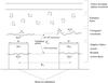 |
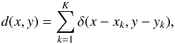
Fig. 1 Sketch of the effect of the turbulence in interferometry. On each telescope pupil
P(r) separated by the baseline
distance B12, the wavefront is affected by a random phase
screen, respectively φ1(r)
and φ2(r). The strength of
the turbulence depends on the parameters
D/r0 where
D is the diameter of the telescope
and r0 is the Fried parameter (Fried 1965), describing the typical size of a coherent cell in the
wavefront. Furthermore, the optical path difference between the two beams is randomly
shifted by the turbulent piston |
Expression of the variance of the phase for the three noise regimes, the detector, photon, and atmospheric regimes, both in the multimode and singlemode cases.
2.1. General description and underlying assumptions
The groundbased interferometer: As sketched in Fig. 1, we consider an interferometer with two telescopes,
separated by the baseline distance B12. We assume that both
telescopes are identical, that is they are described by the same pupil function
P(r) of diameter D, therefore by the
same collecting area ΣP defined as
ΣP = ∫ [ P(r) ] 2dr.
Their transmissions are different however, namely t1 and
t2 respectively. The wavefront over each telescope is
affected by randomly moving phase screens,
φ1(r) and
φ2(r) respectively. The typical cell size
of these turbulent phases is r0 (Fried 1965) and the strength of the turbulence is characterized by the
quantity D/r0. When
Adaptive Optic systems are installed on each telescope, they partially compensate in
real-time the wavefront corrugations of the atmosphere. The correction is not perfect
however, and residual phases  and
and  remain, affecting the two telescopes. Because of
this turbulence, the optical path difference (opd) between the two light paths to the star
through the two telescopes is randomly shifted by the so-called turbulent piston
remain, affecting the two telescopes. Because of
this turbulence, the optical path difference (opd) between the two light paths to the star
through the two telescopes is randomly shifted by the so-called turbulent piston
 , i.e. the phase difference
between the two telescopes averaged over the pupils:
, i.e. the phase difference
between the two telescopes averaged over the pupils:  (1)The
interferogram: A 2-telescope interferogram consists in an incoherent part, which
is the sum of the photometric fluxes coming from both telescopes, and a modulated coherent
part – namely the fringes, which are proportional to the so-called complex coherent flux
(1)The
interferogram: A 2-telescope interferogram consists in an incoherent part, which
is the sum of the photometric fluxes coming from both telescopes, and a modulated coherent
part – namely the fringes, which are proportional to the so-called complex coherent flux
 , which depends on the flux
N (photons per surface unit and per time unit) and on the complex
visibility V12 of the source corresponding to the baseline
frequency
f12 = B12/λ
of the interferometer. λ is the effective wavelength of the
interferogram. The modulation of the fringes can be either temporal, when the opd is
scanned with moving piezo-mirrors (temporal coding), or spatial, when the opd is scanned
with dedicated output pupils, whose separation defines the frequency of the modulation
(spatial coding).
, which depends on the flux
N (photons per surface unit and per time unit) and on the complex
visibility V12 of the source corresponding to the baseline
frequency
f12 = B12/λ
of the interferometer. λ is the effective wavelength of the
interferogram. The modulation of the fringes can be either temporal, when the opd is
scanned with moving piezo-mirrors (temporal coding), or spatial, when the opd is scanned
with dedicated output pupils, whose separation defines the frequency of the modulation
(spatial coding).
Finally, the phase of the interferogram Φ12, that is the phase shift with
respect to the zero opd, originates from the source phase  , a potential instrumental
phase
, a potential instrumental
phase  , which
we will assume equal to zero below1, and the
turbulence piston phase
, which
we will assume equal to zero below1, and the
turbulence piston phase  .
.
2.2. Estimating the interferometric phase and its associated error
Estimating the interferometric phase Φ12 requires us to define and compute
from each interferogram an appropriate complex estimator  of the
complex coherent flux . Several methods are possible
to build this estimator, such as “ABCD” techniques in the image plane (Colavita 1999; Tatulli
et al. 2007) or an analysis in the Fourier plane (Roddier & Lena 1984; Coudé du Foresto
et al. 1997). In any case, the measured phase is then the argument of the complex
estimator :
of the
complex coherent flux . Several methods are possible
to build this estimator, such as “ABCD” techniques in the image plane (Colavita 1999; Tatulli
et al. 2007) or an analysis in the Fourier plane (Roddier & Lena 1984; Coudé du Foresto
et al. 1997). In any case, the measured phase is then the argument of the complex
estimator :
![Mathematical equation: \begin{equation} \Phi_{12} = \mathrm{atan}\left[\frac{\mathrm{Im}\left(\widetilde{F^c_{12}}\right)}{\mathrm{Re}\left(\widetilde{F^c_{12}}\right)}\right]\cdot \end{equation}](/articles/aa/full_html/2010/16/aa13356-09/aa13356-09-eq46.png) (2)In this framework, one
can show that in first approximation, i.e. when the error on is small
compared to its amplitude, the variance of the instantaneous phase (i.e. measured over one
interferogram) can be expressed as (Chelli 1989, see
Eq. (5), case j = k):
(2)In this framework, one
can show that in first approximation, i.e. when the error on is small
compared to its amplitude, the variance of the instantaneous phase (i.e. measured over one
interferogram) can be expressed as (Chelli 1989, see
Eq. (5), case j = k): ![Mathematical equation: \begin{equation} \sigma^2_{\phi} = \frac{1}{2}\frac{{E}\left(\left|\widetilde{F^c_{12}}\right|^2\right)-\mathrm{Re}\left[{E}\left(\widetilde{F^c_{12}}^2\right)\right]}{\left[{E}\left(\widetilde{F^c_{12}}\right)\right]^2}, \label{eq_errphi} \end{equation}](/articles/aa/full_html/2010/16/aa13356-09/aa13356-09-eq48.png) (3)where E
denotes the expected value. Chelli (1989) has also
demonstrated that the variance of the interferometric phase is independent of the object
phase. For the sake of simplicity, we will therefore consider that the source of interest
is centro-symmetric, namely
(3)where E
denotes the expected value. Chelli (1989) has also
demonstrated that the variance of the interferometric phase is independent of the object
phase. For the sake of simplicity, we will therefore consider that the source of interest
is centro-symmetric, namely  .
.
Regardless of the method used to build the estimator from the interferogram, the statistics of the phase will depends on whether the interferometer is using a multimode or a singlemode design. Below, we explore how the atmospheric spatial fluctuations of the turbulent wavefront affect the fringe pattern in multimode and singlemode cases.
2.3. The coherent flux in multimode interferometry
In multimode interferometry, the total flux on the detector remains constant (neglecting scintillation) and the interferograms are created in speckle patterns randomly moving with the fluctuations of the turbulent wavefronts over the two telescopes.
There are two different ways to combine the beams in multimode interferometry (Chelli & Mariotti 1986): whether in the image
plane, a technique which is suited to perform spatial coding of the fringes on the
detector, known as Fizeau (Beckers & Hege
1984) and Michelson (Mourard et al. 1994)
mountings2, or in the pupil plane, which is
commonly used to temporally sample the interferogram through dedicated moving
piezo-electric mirrors (Dyck et al. 1995). In both
cases however, the expression of the coherent flux can be written as (as shown in the
demonstration of Appendices A.3.1 and A.3.2 of this paper and in Appendices A1 and A2 of Buscher et al. 2008):  (4)T12
is the normalized interferometric transfer function resulting of the cross-correlation of
the pupil of the two telescopes, corrugated by the residual atmospheric screen phases
(4)T12
is the normalized interferometric transfer function resulting of the cross-correlation of
the pupil of the two telescopes, corrugated by the residual atmospheric screen phases
 and
and  , (see Fig. 1). It writes:
 ![Mathematical equation: \begin{equation} \label{eq_coupling_multi} T_{12} = \frac{\int [P({\vec r})]^2 \mathrm{e}^{i(\phi^r_1({\vec r})-\phi^r_2({\vec r}))}\mathrm{d}{\vec r}}{\int [P({\vec r})]^2\mathrm{d}{\vec r}}\cdot \end{equation}](/articles/aa/full_html/2010/16/aa13356-09/aa13356-09-eq53.png) (5)As an analogy with
classical AO systems on single-pupil telescopes (see e.g. Fusco & Conan 2004), |T12| 2
can be seen as the instantaneous interferometric Strehl ratio, for
multimode interferometry.
(5)As an analogy with
classical AO systems on single-pupil telescopes (see e.g. Fusco & Conan 2004), |T12| 2
can be seen as the instantaneous interferometric Strehl ratio, for
multimode interferometry.
2.4. The coherent flux in singlemode interferometry
The main property of singlemode devices such as fibers or integrated optic chips is to
perform a spatial filtering of the input wavefront so that only its Gaussian part is
transmitted. As a consequence, a singlemode device turns the input spatial wavefront
fluctuations into intensity fluctuations at the output. With this, each outgoing wavefront
is flat, hence the shape of the interferogram is deterministic, only depending on the
instrumental configuration. The trade-off is that only a fraction of the flux is
transmitted, corresponding to the coherent energy of the turbulent wavefront. The
singlemode instantaneous coherent flux thus takes the form (see Appendix A.4, Eq. (A.38))  (6)where
ρ12(V) is the interferometric coupling
coefficient that depends both on the source extension and on the level of AO correction
(Tatulli et al. 2004, see Eqs. (3), and (A.35), Appendix A.4 of this paper). Focusing on compact sources, that is astrophysical objects
unresolved by a single telescope, ρ12(V)
takes a simple expression of the form
ρ12(V) = ρ0V12ρ12
(Tatulli & Chelli 2005, Eqs. (4–6)). The
coherent flux thus rewrites:
(6)where
ρ12(V) is the interferometric coupling
coefficient that depends both on the source extension and on the level of AO correction
(Tatulli et al. 2004, see Eqs. (3), and (A.35), Appendix A.4 of this paper). Focusing on compact sources, that is astrophysical objects
unresolved by a single telescope, ρ12(V)
takes a simple expression of the form
ρ12(V) = ρ0V12ρ12
(Tatulli & Chelli 2005, Eqs. (4–6)). The
coherent flux thus rewrites: 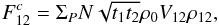 (7)where
ρ12 is independent of the source properties
(7)where
ρ12 is independent of the source properties 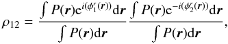 (8)and where
ρ0 is the maximum achievable coupling efficiency, shown to
be ~80% (Shaklan & Roddier 1988), because
of the geometrical mismatch between the telescope Airy disk profile and the Gaussian
profile of the propagated mode.
(8)and where
ρ0 is the maximum achievable coupling efficiency, shown to
be ~80% (Shaklan & Roddier 1988), because
of the geometrical mismatch between the telescope Airy disk profile and the Gaussian
profile of the propagated mode.
Equation (8) has to be compared with Eq. (5). We can see that they are almost similar, but with one major difference: in Eq. (5), the product of the phasors is integrated over the pupil, whereas in Eq. (8), each phasor is first integrated over the pupil, then the product is performed. As noticed by Buscher et al. (2008), this difference is the mathematical expression of the property of spatial filtering.
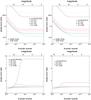 |
Fig. 2 Global performance comparison between multimode and singlemode
interferometry, all sources of noise considered. Top: error of the
phase in multimode (dotted lines) and singlemode (solid lines) as the function of
the number of detected photoevents (per time unit) and K-band
magnitude. For both cases, we can see the three regimes: the detector noise (in
1/N), then (shortly) the photon noise (in
|
Again, |ρ12| 2 – which is equal to 1 for perfect AO correction/absence of atmospheric turbulence – can be seen by as the instantaneous interferometric Strehl ratio, but for the singlemode case.
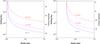 |
Fig. 3 Limiting flux as a function of the Strehl ratio (detector noise regime case) for turbulence strengths of D/r0 = 8 (left) and D/r0 = 2 (right). Plots are shown for an unresolved (V = 1), fairly resolved (V = 0.5), and fully resolved (V = 0.1) source, respectively. Curves are going by pair for singlemode (solid lines) and multimode (dotted lines) cases. The fixed parameters have the same values as previous figures. |
3. Performance comparison
3.1. Phase noise
From Eqs. (3–7), we derive the expression of the error of the phase for both
singlemode and multimode cases, as developed in Appendix A. We show that the variance of the interferometric phase can be decomposed as
the quadratic sum of three terms, corresponding to the detector, photon, and atmospheric
regimes:  (9)where the detail
of each term is given in Table 1. The phase error
depends on parameters coming from the source and the instrument, which we recall here:
N is the number of incoming photons per surface unit and per time unit,
|V12| is the amplitude of the visibility,
t1 and t2 are the transmissions
of both telescopes, Npix is the number of pixels to sample the
interferogram, σdet is the detector noise. The phase error
also depends on atmospheric terms: the long exposure Strehl ratio
(9)where the detail
of each term is given in Table 1. The phase error
depends on parameters coming from the source and the instrument, which we recall here:
N is the number of incoming photons per surface unit and per time unit,
|V12| is the amplitude of the visibility,
t1 and t2 are the transmissions
of both telescopes, Npix is the number of pixels to sample the
interferogram, σdet is the detector noise. The phase error
also depends on atmospheric terms: the long exposure Strehl ratio
 and its associated
coherent energy
and its associated
coherent energy  where
where  is the
variance of the residual phase of a single telescope (Noll
1976), and of the phase structure function with partial AO correction
is the
variance of the residual phase of a single telescope (Noll
1976), and of the phase structure function with partial AO correction
 as modelled in Appendix D.
Figure 2 (top) shows the multimode and singlemode
phase error as a function of the number of incoming photoevents (alternatively, source
K-band magnitude), for different levels of AO correction (i.e.
different Strehl ratios). In a general way, the behavior of the error is similar in both
cases: at low fluxes, the detector noise dominates with a slope of the error in
1/N, then it goes through a (short) photon noise
regime in  and eventually reaches a plateau for the brightest sources due to speckle noise – analog
to the one known in the case of the visibility (Goodman
1985; Tatulli et al. 2004), which limits
the ultimate precision on the phase. Note that in order to keep the phase noise below
reasonable levels, that is smaller than 1 radian, it is mandatory to equip interferometers
with AO systems, to ensure at least a low-order correction of the turbulent phase,
providing Strehl ratios greater than ~0.1 for
D/r0 = 8 and ~0.5 for
D/r0 = 2.
and eventually reaches a plateau for the brightest sources due to speckle noise – analog
to the one known in the case of the visibility (Goodman
1985; Tatulli et al. 2004), which limits
the ultimate precision on the phase. Note that in order to keep the phase noise below
reasonable levels, that is smaller than 1 radian, it is mandatory to equip interferometers
with AO systems, to ensure at least a low-order correction of the turbulent phase,
providing Strehl ratios greater than ~0.1 for
D/r0 = 8 and ~0.5 for
D/r0 = 2.
Going into greater detail, Fig. 2 (bottom) shows the ratio of the error of the multimode phase by the error of the singlemode phase as a function of the number of photoevents. Clearly, two different behaviors occur if we are considering a photon-starved or a photon rich regime, as discussed below.
3.2. Low-light level regime – limiting magnitude
For faint sources, the phase error is dominated by the detector noise σdetφ. The comparison between both multimode and singlemode cases is not straightforward however because the number of pixels required to sample the fringes is specific to each technique, and depends on the chosen combination scheme. Let us first review here the possible technical solutions:
Multimode – (image plane) multiaxial combination: Here, each speckle in which the interferograms are formed must be sampled correctly, that is it must be crossed by at least two pixels (Chelli & Mariotti 1986). Then, if we take the whole image of size λ/r0, the total number of pixels required becomes Npix = 2D/r0. As a consequence, Npix is dependent on the turbulence, in this combination mode. In the case of the VLTI at Cerro Paranal, the average r0 is ≃1m in the K-band, which gives turbulence strengths of D/r0 ≃ 8 and D/r0 ≃ 1.8 for the UTs (D = 8 m) and ATs (D = 1.8 m). This corresponds to a number of pixels that can vary quite a lot with the strength of the turbulence, Npix = 16 (UTs) and Npix = 4 (ATs) respectively.
Multimode – (pupil plane) coaxial combination: Providing that the interferogram is scanned faster than the coherent time of the atmosphere in order to “freeze” the fringes, the minimum number of pixels to obtain full information on the temporal interferogram is 3, which corresponds to the 3 degrees of freedom: incoherent flux, fringe amplitude, and phase. However, instead of this “ABC” scheme with 120 degrees between the three channels, it is frequently more practical to implement an “ABCD” scheme with 90 degree phase shifts, hence requiring 4 pixels. Note that in the framework of phase tracking, it is also possible to only measure the sine component of the fringe with an “AC” scheme with 180 degrees between the two channels. In any case, the number of pixels needed in a coaxial pupil plane combiner is between 2 and 4.
Singlemode – multiaxial combination: Contrary to the multimode/multiaxial combination, the number of pixels here is independent of the turbulence, because the shape and frequency of the interferogram are fixed by the design of the beam combiner. Typically, the interferogram consists in a sinusoidal signal with a frequency defined by the separation of the output pupils (the so-called coding frequency), and where its amplitude is modulated by the Gaussian envelope of the singlemode device. Tatulli & LeBouquin (2006) have shown that the optimum number of pixels that respects the Shannon criterion (>2 pixels per fringe) and prevents an overlapping of the photometric and interferometric peaks in the Fourier plane is Npix = 10.
Singlemode – coaxial combination: As in the coaxial multimode case, one merely needs to sample the interferogram with respect to the 3 degrees of liberty here. As a result, the number of pixels is again between 2 and 4. Note that instead of the usual temporal coding, fringes can be scanned simultaneously thanks to “ABCD-like” integrated chip devices (Benisty et al. 2009).
As a consequence, coaxial schemes – both in multimode and singlemode cases – appear more appropriate, because they are using substantially fewer pixels than multiaxial ones. We remark however that these conclusions apply in the framework of fringe tracking where pair-wise combinations are favored. They may differ in the context of an interferometric imaging instrument where an important number of baselines is involved. Below we will consider coaxial combiners with Npix = 4, corresponding to the standard “ABCD” sampling.
As multimode and singlemode fringe trackers finally require the same number of pixels, a
straightforward comparison of the expressions of the detector noise shows that multimode
combiners will in this regime achieve a slightly better performance by a factor of
1/ρ0, because singlemode spatial filters
cannot transmit 100% of the flux for the geometrical reasons mentioned in previous
sections. If we define the limiting magnitude3 such
as the error of the phase to be equal to 1 rad, which – apart from very low AO correction
levels – occurs in this detector noise regime, the corresponding limiting flux is given by
![Mathematical equation: \begin{equation} K_{\rm lim}^{[\mathrm{multi,single}]} = \frac{\sqrt{2}\sqrt{N_{\rm pix}}\sigma_{\rm det}}{[1,\rho_0]V_{12}\mathrm{e}^{-\sigma^2_{\phi_{\rm r}}}}, \end{equation}](/articles/aa/full_html/2010/16/aa13356-09/aa13356-09-eq102.png) (10)with the factor 1 or
ρ0 depending whether we are using multimode or singlemode
interferometers. As illustrated by Fig. 3, the gain
in limiting magnitude for multimode combiners is ~0.25 magnitude.
(10)with the factor 1 or
ρ0 depending whether we are using multimode or singlemode
interferometers. As illustrated by Fig. 3, the gain
in limiting magnitude for multimode combiners is ~0.25 magnitude.
3.3. High-light level regime: the speckle noise
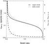 |
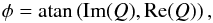
Fig. 4 Phase speckle noise as a function of the Strehl ratio for both singlemode (solid line) and multimode (dotted line) cases, with D/r0 = 8. The ratio between the multimode and the singlemode phase errors is plotted in dashed line (y-axis on the right side). |
In the photon-rich regime, the speckle noise dominates and the error on the interferometric phase reaches a plateau, that is, is not dependent on the flux of the source anymore. As illustrated by Fig. 4, singlemode interferometers always provide a lower phase error than multimode ones, emphasizing the remarkable properties of spatial filtering of the turbulent wavefront by singlemode devices. This behavior was already noticed by Tatulli et al. (2004) for the estimate of the squared visibility, showing that the so-called modal speckle noise of the visibility was, for a given AO correction, always lower than classical speckle noise of multimode interferometers. The concept of modal speckle noise can also be applied for the singlemode interferometric phase. However, at the difference of the squared visibility for which the modal speckle noise is 0 for a point source, the phase modal speckle noise always exists, independently of the size of the source.
Note that the gain of using singlemode schemes is all the more important than the level of correction is low. If for a fairly good correction with a Strehl ratio above 20%, the difference remains marginal with a factor ~1−1.5 between the singlemode and multimode phase error, the situations where bright sources are observed with low/none AO correction will highly benefit from singlemode interferometers. In these cases the precision of the phase can increase by at least a factor of 2 and much more when using spatial filtering of the corrugated wavefront with a typical Strehl ratio below 10%. This is a typical counter-intuitive example where it is more profitable to loose a substantial part of the flux and keep only the coherent part of the perturbed wavefronts than conserving the whole flux at the price of introducing additional atmospheric noise.
4. Application to fringe tracking
In this section, we apply the formalism developed above in the context of on-axis and off-axis fringe tracking, that is when the phase is estimated and compensated in real time to stabilize the fringes on the detector. We focus on the relative performance of fringe tracking systems using either multimode or singlemode schemes.
4.1. Coherent integration
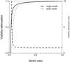 |
Fig. 5 Long exposure visibility attenuation owing to the atmospheric noise of the measurement of the phase, as a function of the Strehl ratio for multimode (dotted line) and singlemode (solid line) systems, with D/r0 = 8. The ratio of the attenuation between singlemode and multimode is plotted in a dashed line (y-axis on the right side). |
Centering the fringes in real time allows us to perform coherent integration of the
signal, that is to integrate on time scales much longer than the coherence time of the
atmosphere. However, the estimated piston used for the opd correction is affected by a
random measurement error ϵ(t). As a result, the
interferogram is not perfectly centered and is still moving with an excursion depending on
the statistics of the noise. If the interferograms are integrated over a time that is long
enough for the realizations of the random error ϵ(t) to
span all the range of its probability law, then, by rules of ergodicity, the visibility
will be affected by a loss of contrast4, which writes
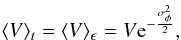 (11)where
⟨ ⟩ ϵ is the ensemble average over the realizations of
the noise, and
(11)where
⟨ ⟩ ϵ is the ensemble average over the realizations of
the noise, and  is the variance of this noise
as computed in Sect. 3.1. Hence, for long integration
times, an attenuation of the coherent flux (equivalently of the visibility) by a factor
is the variance of this noise
as computed in Sect. 3.1. Hence, for long integration
times, an attenuation of the coherent flux (equivalently of the visibility) by a factor
 is introduced by the instantaneous turbulent phase, which is corrected only to the
precision of its estimation. This bias therefore depends on whether singlemode or
multimode fringe tracking is used.
is introduced by the instantaneous turbulent phase, which is corrected only to the
precision of its estimation. This bias therefore depends on whether singlemode or
multimode fringe tracking is used.
For the high-light level regime, where the fringe tracking is mostly expected to work, Fig. 5 shows the attenuation of the visibility as a function of the Strehl ratio for both singlemode and multimode systems. We can see that acceptable loss of contrast, typically ≳ 0.8, is achieved as soon as moderate AO corrections with Strehl ≳ 0.1 (for D/r0 = 8) are provided. On the contrary, for a lower performance of the AO system, the attenuation coefficient drops rapidly and the advantage of tracking the fringes is lost because of the uncompensated turbulent fluctuations of the phase over the pupils.
One important conclusion to draw is that for a given AO correction, the visibility attenuation induced by the noise of the phase is always smaller when using singlemode fringe tracking systems instead of multimode ones. In other words, the maximum achievable atmospheric contrast is always higher using singlemode fringe tracker than with multimode systems. This is especially true for low AO correction cases where the attenuation can become twice as large and more, as shown in Fig. 5.
4.2. Phase jumps
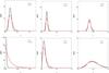 |
Fig. 6 Density probability of the multimode instantaneous Strehl ratio (I = |T12| 2, red lines) and singlemode one (I = |ρ12| 2, black lines) for various levels of AO correction and turbulence strengths. Top: constant turbulence strength D/r0 = 8 and the number of corrected Zernike are, from left to right, nz = 10,15,30. Bottom: constant AO correction nz = 3 (tip-tilt only), with various turbulence strengths, from left to right D/r0 = 8,4,2. |
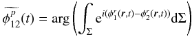
![Mathematical equation: \begin{equation} \phi^p_{12}(t) = \int_{\Sigma} [\phi^r_1({\vec r},t) - \phi^r_2({\vec r},t)] \mathrm{d}{\Sigma}, \label{eq_pistonphase} \end{equation}](/articles/aa/full_html/2010/16/aa13356-09/aa13356-09-eq119.png) (12)following the
formalism of Buscher et al. (2008, see Eq. (6)),
where dΣ is an elemental within the aperture Σ.
(12)following the
formalism of Buscher et al. (2008, see Eq. (6)),
where dΣ is an elemental within the aperture Σ.
As first brought up by these authors, the practical estimate  of this piston phase is
performed by taking the argument of the complex phasor averaged over the pupils, that is
of this piston phase is
performed by taking the argument of the complex phasor averaged over the pupils, that is
 (13)in
the multimode case, and
(13)in
the multimode case, and 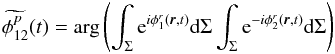 (14)in
the singlemode one.
(14)in
the singlemode one.
By comparing Eq. (12) to Eqs. (13, 14) we can see that the true piston phase and the estimated one
 are
literally not the same, unless when there is no phase fluctuation (i.e. no turbulence or a
perfect correction of the wavefronts) across the apertures.
are
literally not the same, unless when there is no phase fluctuation (i.e. no turbulence or a
perfect correction of the wavefronts) across the apertures.
When considering a small amount of fluctuations
δφ12(r,t)
such as 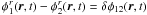 , a
Taylor expansion of Eqs. (13, 14) can show that and will then
deviate roughly as
∫Σ [ δφ12(r,t) ] 3dΣ
(Buscher et al. 2008). But if these fluctuations
are high (typically above 1 radian), there can be strong differences between the piston
phase and the argument of the complex phasor. More precisely, strong divergences are
occurring when the complex phasor has a very small amplitude and eventually crosses the
origin of the complex plane. Then rapid phase jumps of the argument of the phasor can be
experienced, whereas these jumps are not seen in the piston phase. As a consequence the
correction performed by the fringe tracker may be highly wrong and fringes potentially
lost, especially if the science camera is working at a different wavelength than that of
the fringe tracker (Buscher et al. 2008), as is the
case e.g. for the FINITO instrument (fringe tracking in H-band and
correction in K-band, Gai et al.
2004; Le Bouquin et al. 2008).
, a
Taylor expansion of Eqs. (13, 14) can show that and will then
deviate roughly as
∫Σ [ δφ12(r,t) ] 3dΣ
(Buscher et al. 2008). But if these fluctuations
are high (typically above 1 radian), there can be strong differences between the piston
phase and the argument of the complex phasor. More precisely, strong divergences are
occurring when the complex phasor has a very small amplitude and eventually crosses the
origin of the complex plane. Then rapid phase jumps of the argument of the phasor can be
experienced, whereas these jumps are not seen in the piston phase. As a consequence the
correction performed by the fringe tracker may be highly wrong and fringes potentially
lost, especially if the science camera is working at a different wavelength than that of
the fringe tracker (Buscher et al. 2008), as is the
case e.g. for the FINITO instrument (fringe tracking in H-band and
correction in K-band, Gai et al.
2004; Le Bouquin et al. 2008).
It is therefore important to know the probability of phase jumps to occur in order to ensure an observational/instrumental context in which these events are avoided as much as possible. So far, the conclusions about this point are not clear: if Tubbs (2005) implied that spatial filtering could be the source of these anomalies, Buscher et al. (2008) on the contrary argues that AO correction and most of all spatial filtering help to reduce these singularities. All the previous analysis were however based only on simulations. We propose here a theoretical analysis of this phenomenon. We emphasize that our analysis focuses on the rate of occurrence of phase jumps, as defined above. We do not study the consequences of these phase jumps in terms of an effective loss of fringe tracking. Such a causality will depend on the system (e.g. single wavelength vs. multiple spectral channels methods) used to practically estimate and correct the opd. Considering that a phase jump would systematically induce a failure in the fringe tracking system therefore corresponds to the worst case scenario.
That the coherent flux drops to zero because of turbulent phase fluctuation depends on
whether the interferometric transfer function |T12| for
multimode systems or the interferometric coupling coefficient
|ρ12| in the singlemode case, drops to zero. We thus aim
here to establish the probability density of these quantities, and study how likely it is
for them to take very low values. Canales & Cagigal
(1999) have studied the distribution of speckle statistics in presence of partial
AO correction for mono-pupil telescopes. They have shown that the density probability
dp(I) of the intensity I at the center of the image –
that is by definition, the instantaneous Strehl ratio – follows a Rician statistics of the
form  (15)where
a2 and σ2 depend on the first
and second order moments of the real and imaginary part of the complex phasor describing
the AO-corrected turbulent wavefront. Note that this analytical definition of the density
probability implicitly assumes a time-constant r0 to
characterize the turbulence. This hypothesis is the limitation of our model because
r0 may actually vary on time scales of minutes and shorter,
which leads to brief episodes of very small r0 that would trip
up AO systems and lead to a very low Strehl ratio for a brief period of time. However,
modelling this effect requires more complex and heavy simulations of partially
AO-corrected turbulence, which is beyond the scope of this paper.
(15)where
a2 and σ2 depend on the first
and second order moments of the real and imaginary part of the complex phasor describing
the AO-corrected turbulent wavefront. Note that this analytical definition of the density
probability implicitly assumes a time-constant r0 to
characterize the turbulence. This hypothesis is the limitation of our model because
r0 may actually vary on time scales of minutes and shorter,
which leads to brief episodes of very small r0 that would trip
up AO systems and lead to a very low Strehl ratio for a brief period of time. However,
modelling this effect requires more complex and heavy simulations of partially
AO-corrected turbulence, which is beyond the scope of this paper.
We emphasized in Sect. 2 that |T12| 2 and |ρ12| 2 represent the instantaneous interferometric Strehl ratio for the multimode and singlemode cases, respectively. Therefore, by straightforward analogy with an interferometric pupil instead of a monolithic one, we can show that I = |T12| 2 and I = |ρ12| 2 are also following a Rician distribution. The parameters a2 and σ2 relative to both instantaneous interferometric Strehl ratio can be directly derived from the formalism of the previous section, and their expressions are given in Table B.1 of Appendix B.
 |
Fig. 7 Left: probability for the instantaneous interferometric Strehl ratio I to be lower than the value ϵ for the tip-tilt correction only, for different strengths of turbulence D/r0 = 8,4,2 (respectively in blue, magenta and red), for the multimode (dotted line) and singlemode (solid line) cases. Right: multimode versus singlemode probability ratio. |
High-order AO correction: first, we can see that as soon as
moderate AO correction is applied – roughly a few tens of modes or a Strehl ratio ≳ 0.3,
the probability density displays a bell shape, which becomes narrower with a higher AO
correction, and the probability that |T12| or
|ρ12| goes to very low values is null (typically, for
nz = 15 and
D/r0 = 8, the probability for the
interferometric instantaneous Strehl ratio to be < 0.01 is
< 10-9, and < 0.05 is
< 0.02%), emphasizing again the relevance of associating
high-performance AO systems to fringe tracking devices, whether the wavefront is spatially
filtered or not. We note that the intensity mean value
(⟨ I ⟩ = 2σ2 + a2)
is systematically slightly higher in the singlemode case and the dispersion
( ) slightly smaller. The difference is
not critical however.
) slightly smaller. The difference is
not critical however.
Low-order AO correction: for low-order AO such as tip-tilt correction only, the situation is fairly different. The shape of the distribution has changed, peaking at zero for strong turbulence with high values of D/r0 ≳ 5. The probability to have a very low value of the intensity is thus significant, and events such as phase jumps are likely to happen. In other words, tip-tilt correction is an insufficient order correction to exclude these events.
Figure 7 displays the probability P(I) for the instantaneous interferometric Strehl ratio to reach values close to zero (i.e. P(I < ϵ) with ϵ very small) for different strengths of the atmospheric turbulence. We can see that for strong turbulence (D/r0 ≳ 5), the probability P(I) < ϵ is always higher in the singlemode case. In these cases we expect phase jumps to occur more frequently with the singlemode fringe tracker, because the likelihood that two speckles are simultaneously entering the singlemode fibers of the two telescopes is weak. However, this does not mean that phase jumps cannot occur often with multimode fringe tracker too. As an example the probability to have instantaneous interferometric Strehl lower than 0.01 in the multimode case is ~78% for D/r0 = 8, whereas it is 100% in the singlemode. In other words, regardless of the multimode versus singlemode issue, one should never consider to perform fringe tracking with big telescope apertures associated with solely the tip-tilt correction.
For weak turbulence (roughly D/r0 ≲ 5, Fig. 6, bottom middle and right), the distribution starts to look like a bell shape again, but this time with a slight probability to have a zero intensity. But as shown in Fig. 7 this probability is now higher in the multimode case, because only a few and big speckles are present in the images. Indeed, this case is the one treated by Buscher et al. (2008, see Fig. 4, with D/r0 = 4 in his simulations, and we come to the same conclusion as he: in these conditions, spatial filtering lets the number of phase jump events decrease. We emphasize here though that this statement is true only for cases of moderate turbulence strength.
Application to the VLTI: We recall that at Paranal the average r0 is ~1 m in the K-band, which gives turbulence strengths of D/r0 ~ 8 and D/r0 ~ 1.8 for the UTs and ATs, respectively. The UTs come with high-order Adaptive Optic systems (MACAO, Arsenault et al. 2004), therefore one can equally choose multimode or singlemode fringe tracking schemes because (i) phase jumps are unlikely to occur in any case; and (ii) multimode and singlemode fringe trackers will provide the same robustness to eventual phase jumps. For ATs where tip-tilt correction is currently provided, the likelihood to endure phase jumps is also very low. But to maximize the stability of their fringe tracking system, it still seems appropriate to accompany the ATs with singlemode spatial filtering devices because the probability to undergo these phase jumps remains roughly 10 times lower (see Fig. 7, right). Alternatively, providing higher order AO correction to ATs will fix the phase jump issue.
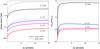 |
Fig. 8 Left: astrometric phase error caused by atmospheric turbulence, as the function of the angular distance Δα between the source and the reference star for both singlemode (solid lines) and multimode (dotted lines). Right: ratio of the multimode versus the singlemode astrometric error. Results are shown for various AO correction levels as described in the figures above. We have assumed one single turbulent layer located at h = 10 km. |
4.3. Phase referencing – astrometry
The interest of phase referencing instruments such as PRIMA, which was recently installed on the VLTI (Delplancke et al. 2000), is (i) to provide sub-microarcsecond precision astrometry, allowing e.g. the detection of the presence of a faint companion (extrasolar planet) around the central star (Launhardt et al. 2008); and (ii) to drastically increase the limiting magnitude of the interferometer by locking the fringes of the (possibly faint) science object on a simultaneously observed bright off-axis reference star whose phase is used as reference (Sahlmann et al. 2008). This method requires that the nearby reference star is close enough – typically in the isoplanatic patch – in order to assume that both the wavefront of the source and the reference are identically perturbed by the atmospheric turbulence. Strictly speaking, this assumption is not true because the optical paths of the two stars are different, crossing different part of the atmosphere in the turbulent layers. As a result, the loss of correlation between the two wavefronts will lead to an atmospheric noise on the astrometric phase, which will lower the ultimate performance of this method.
We call respectively φs, and
 , the phase of the
astrophysical target and the phase estimated from the off-axis reference source, located
at an angular distance Δα of the science object, and where we assume for
the sake of simplicity a single turbulent layer located at an height h
from the ground. The astrometric phase is then simply defined by
, the phase of the
astrophysical target and the phase estimated from the off-axis reference source, located
at an angular distance Δα of the science object, and where we assume for
the sake of simplicity a single turbulent layer located at an height h
from the ground. The astrometric phase is then simply defined by
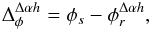 (16)and its associated
error writes
(16)and its associated
error writes 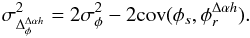 (17)Equation (17) tells us that the noise of the astrometric
phase increases as long as the correlation between the two turbulent wavefronts
(17)Equation (17) tells us that the noise of the astrometric
phase increases as long as the correlation between the two turbulent wavefronts
 decreases, that is as long as the spatial
distance Δαh between both turbulent phase screens is getting higher. The
quantitative effect of the separation between the star and its reference on the
interferometric narrow-angle astrometric error has already been studied by Shao & Colavita (1992), and we refer the
readers to their paper for more details. In our analysis, we focus on the relative
performance of astrometry between the multimode and singlemode scheme, studying how
spatial filtering of the wavefronts will impact on the astrometric error, as developed in
Appendix C.
decreases, that is as long as the spatial
distance Δαh between both turbulent phase screens is getting higher. The
quantitative effect of the separation between the star and its reference on the
interferometric narrow-angle astrometric error has already been studied by Shao & Colavita (1992), and we refer the
readers to their paper for more details. In our analysis, we focus on the relative
performance of astrometry between the multimode and singlemode scheme, studying how
spatial filtering of the wavefronts will impact on the astrometric error, as developed in
Appendix C.
For sake of simplicity we have assumed in the following one single turbulent layer located at h = 10 km as it is the strongest layer at the Cerro Paranal site (Masciadri et al. 1999). There is also a strong layer very close to the ground at around 20 m (Martin et al. 2000) but that only marginally contributes to the phase decorrelation, because the linear distance at stake is 500 times smaller than the one at the high altitude layer. Figure 8 (left) shows the evolution of the astrometric error as a function of the angular distance between the source and the reference for both the singlemode and multimode scheme.
Large field of view: when the reference source is farther away than about
≃1′′ from the astrophysical object of interest, we can see that spatial
filtering allows us to increase the precision of the astrometric phase. The improvement is
better when the AO correction is low, reaching a factor of ~4 without AO correction, as
emphasized by Fig. 8 (right). This argues in favor of
using spatial-filtering elements in the design of astrometric instruments with a large
field of view (FOV), as was chosen for PRIMA (FOV ≃ 30′′). Looking at more
details, one can notice that the phase tends asymptotically toward a plateau, from an
angular separation of ~10′′ that roughly corresponds to the isoplanatic angle
of Paranal in the K-band5. Indeed,
from this angle wavefronts can be considered as uncorrelated and the astrometric error
converges to  , which does not depend on the
separation Δα any longer. As a consequence in this regime (i.e.
Δα ≳ 10′′) the astrometric phase error ratio can be
approximated by the speckle phase error ratio, which we already discussed in Sect. 3.3.
, which does not depend on the
separation Δα any longer. As a consequence in this regime (i.e.
Δα ≳ 10′′) the astrometric phase error ratio can be
approximated by the speckle phase error ratio, which we already discussed in Sect. 3.3.
Narrow field of view: on the contrary, when wavefronts are still strongly correlated (Δα ≲ 1′′), the performance of singlemode astrometry is slightly poorer (by a factor ~1 to ~1.5) than that of multimode astrometry, the error of the latter decreasing faster as the separation between the astrophysical source and the reference shrinks to zero. By smoothing the turbulent wavefronts across the apertures, spatial filtering is indeed lowering the effect of the strong correlation between the wavefronts. This situation concerns the cases for which the reference is very close to the star, like GRAVITY, the second generation of astrometric instruments of the VLTI (Gillessen et al. 2006, FOV ≃ 2′′).
5. Summary and conclusions
We provided a theoretical formalism that allows us to derive the error of the interferometric phase both for singlemode and multimode interferometry. From these derivations, we demonstrated that:
-
Contrarily to a widespread idea, losing flux by injecting the lightinto singlemode spatial filters is not a performance killer forestimating the phase. Indeed singlemode interferometryprovides a better performance than that of multimodeinterferometry, unless the interferometer is working in thedetector noise regime (faint sources). Then multimodeinterferometry is slightly better, providing a phase error smallerby a factorρ0 ≃ 0.8, which is the maximum fraction of flux that can be injected in singlemode devices.
-
In cases of bright source observations, spatial filtering is shown to be very efficient, especially when the AO correction of the turbulent wavefronts is poor or absent. In these situations, the precision of the singlemode interferometric phase is better than that of the multimode one by a factor of 2 and more when the Strehl is below 10%.
-
Singlemode interferometry also proves to be more robust to the turbulence of both locking and coherently integrating the fringes and providing a better astrometric precision when using phase referencing techniques, except for narrow fields of view (FOV ≲ 1′′).
In conclusion, from a theoretical point of view and contrarily to a widespread opinion, singlemode fringe tracking should be seriously considered as an advantageous technical solution. Furthermore, the astronomers should realize that the many gains of singlemode interferometry (flexibility of the solutions, robustness to the alignment, less optical elements,...) may significantly compensate a modest and limited loss of performance in the faint sources case compared to multimode interferometry solutions. This is all the more true because the detectors should soon evolve to reach photon counting capability.
Considering a non zero instrumental phase would only introduce an
extra shift of the interferogram, but would not affect the performance of the
interferometer, as long as this instrumental phase is stable or calibratable.
In the Fizeau combination, the output pupil is homothetic to the entrance one, whereas in the Michelson scheme this property is not conserved.
Note that the definition of the limiting magnitude depends on the estimator chosen to measure the phase. Here the interferometric phase is merely estimated at the baseline frequency f12, which is at the top of the interferometric peak (see Appendices A.3 and A.4). If a different estimator is used, like integrating the high frequency peak over the frequency range [f12 − D/λ,f12 + D/λ] (see e.g. Roddier & Lena 1984; Mourard et al. 1994, in the case of the squared visibility estimators), the expression, and therefore the value of the limiting magnitude will change accordingly.
For the sake of simplicity, we assume here that the phase is instantaneously compensated, hence we do not take into account the delay of the fringe tracking loop between the measurement of the phase and its correction. The problem of time delay, which is independent of the multimode or singlemode nature of the fringe-tracking system, is treated in Conan et al. (2000).
Considering the measurements of Martin et al. (2000), who have found an average isoplanatic angle of ~1.9′′ in the visible, and recalling that it evolves with wavelength as λ1.2 (Shao & Colavita 1992).
Acknowledgments
The authors are grateful to the anonymous referee, whose careful and thorough review of the text and theoretical formalism helped them improve the papers clarity and quality considerably.
References
- Arsenault, R., Donaldson, R., Dupuy, C., et al. 2004, in SPIE Conf. Ser., 5490, ed. D. Bonaccini Calia, B. L. Ellerbroek, & R. Ragazzoni, 47 [Google Scholar]
- Beckers, J. M., & Hege, E. K. 1984, in Very Large Telescopes, their Instrumentation and Programs, ed. M.-H. Ulrich, & K. Kjaer, IAU Colloq. 79, 279 [Google Scholar]
- Benisty, M., Berger, J., Jocou, L., et al. 2009, A&A, 498, 601 [NASA ADS] [CrossRef] [EDP Sciences] [Google Scholar]
- Berger, D. H., Monnier, J. D., Millan-Gabet, R., et al. 2008, in Presented at the Society of Photo-Optical Instrumentation Engineers (SPIE) Conf., 7013 [Google Scholar]
- Buscher, D. 1988, MNRAS, 235, 1203 [NASA ADS] [CrossRef] [Google Scholar]
- Buscher, D. F., Young, J. S., Baron, F., & Haniff, C. A. 2008, in Presented at the Society of Photo-Optical Instrumentation Engineers (SPIE) Conf., 7013 [Google Scholar]
- Canales, V. F., & Cagigal, M. P. 1999, Appl. Opt., 38, 766 [NASA ADS] [CrossRef] [PubMed] [Google Scholar]
- Chelli, A. 1989, A&A, 225, 277 [NASA ADS] [Google Scholar]
- Chelli, A., & Mariotti, J. M. 1986, A&A, 157, 372 [Google Scholar]
- Colavita, M. M. 1999, PASP, 111, 111 [NASA ADS] [CrossRef] [Google Scholar]
- Conan, J. 1994, Ph.D. Thesis, Université Paris XI Orsay [Google Scholar]
- Conan, R., Ziad, A., Borgnino, J., Martin, F., & Tokovinin, A. A. 2000, in SPIE Conf., 4006, ed. P. Léna & A. Quirrenbach, 973 [Google Scholar]
- Coudé du Foresto, V., Ridgway, S., & Mariotti, J.-M. 1997, A&AS, 121, 379 [NASA ADS] [CrossRef] [EDP Sciences] [Google Scholar]
- Coudé du Foresto, V., Faucherre, M., Hubin, N., & Gitton, P. 2000, A&AS, 145, 305 [Google Scholar]
- Delplancke, F., Leveque, S. A., Kervella, P., Glindemann, A., & D’Arcio, L. 2000, in SPIE Conf., 4006, ed. P. Léna & A. Quirrenbach, 365 [Google Scholar]
- Dyck, H. M., Benson, J. A., Carleton, N. P., et al. 1995, AJ, 109, 378 [NASA ADS] [CrossRef] [Google Scholar]
- Fried, D. L. 1965, J. Opt. Soc. Am. (1917–1983), 55, 1427 [CrossRef] [Google Scholar]
- Fusco, T., & Conan, J.-M. 2004, J. Opt. Soc. Am. A, 21, 1277 [NASA ADS] [CrossRef] [Google Scholar]
- Gai, M., Menardi, S., Cesare, S., et al. 2004, in SPIE Conf., 5491, ed. W. A. Traub, 528 [Google Scholar]
- Gillessen, S., Perrin, G., Brandner, W., et al. 2006, in SPIE Conf., 6268 [Google Scholar]
- Goodman, J. W. 1985, Statistical optics (New York: Wiley-Interscience), 567 [Google Scholar]
- Jurgenson, C. A., Santoro, F. G., Baron, F., et al. 2008, in SPIE Conf. Ser., 7013 [Google Scholar]
- Launhardt, R., Queloz, D., Henning, T., et al. 2008, in SPIE Conf. Ser., 7013 [Google Scholar]
- Le Bouquin, J.-B., Abuter, R., Bauvir, B., et al. 2008, in SPIE Conf. Ser., 7013 [Google Scholar]
- Martin, F., Conan, R., Tokovinin, A., et al. 2000, A&AS, 144, 39 [Google Scholar]
- Masciadri, E., Vernin, J., & Bougeault, P. 1999, A&AS, 137, 203 [Google Scholar]
- Mège, J.-M. 2002, Ph.D. Thesis [Google Scholar]
- Mège, P., Malbet, F., & Chelli, A. 2003, in SPIE Conf., 4838, ed. W. A. Traub, 329 [Google Scholar]
- Mourard, D., Tallon-Bosc, I., Rigal, F., et al. 1994, A&A, 288, 675 [NASA ADS] [Google Scholar]
- Noll, R. J. 1976, J. Opt. Soc. Am. (1917–1983), 66, 207 [NASA ADS] [CrossRef] [Google Scholar]
- Roddier, F. 1979, J. Opt., 10, 299 [NASA ADS] [CrossRef] [Google Scholar]
- Roddier, F., & Lena, P. 1984, J. Opt., 15, 171 [NASA ADS] [CrossRef] [Google Scholar]
- Sahlmann, J., Abuter, R., Di Lieto, N., et al. 2008, in SPIE Conf. Ser., 7013 [Google Scholar]
- Shaklan, S., & Roddier, F. 1988, Appl. Opt., 27, 2334 [NASA ADS] [CrossRef] [PubMed] [Google Scholar]
- Shao, M., & Colavita, M. M. 1992, A&A, 262, 353 [NASA ADS] [Google Scholar]
- Tatulli, E., & Chelli, A. 2005, J. Opt. Soc. Amer. A, 22, 1589 [NASA ADS] [CrossRef] [Google Scholar]
- Tatulli, E., & LeBouquin, J. 2006, MNRAS, 368, 1159 [NASA ADS] [CrossRef] [Google Scholar]
- Tatulli, E., Mège, P., & Chelli, A. 2004, A&A, 418, 1179 [NASA ADS] [CrossRef] [EDP Sciences] [Google Scholar]
- Tatulli, E., Millour, F., Chelli, A., et al. 2007, A&A, 464, 29 [NASA ADS] [CrossRef] [EDP Sciences] [Google Scholar]
- Tubbs, R. 2005, Appl. Opt., 44, 6253 [NASA ADS] [CrossRef] [PubMed] [Google Scholar]
- Vannier, M., Petrov, R. G., Lopez, B., & Millour, F. 2006, MNRAS, 367, 825 [NASA ADS] [CrossRef] [Google Scholar]
Appendix A: Computation of the interferometric phase error
A.1. General formalism
We here recall Goodman’s approach (Goodman
1985), which is based on a continuous model of detection process, where the
recorded signal (i.e. the interferogram) can be represented as
 (A.1)and its Fourier
transform as
(A.1)and its Fourier
transform as 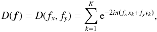 (A.2)where the
position (xn) and the number of photoevents
(per time unit) (K) are statistical processes with probability laws
depending on the intensity distribution
I(x). To take also into account the
detector noise, one needs to add Gaussian additive noise (ϵ) to the
previous equation (Tatulli et al. 2004; Tatulli & Chelli 2005):
(A.2)where the
position (xn) and the number of photoevents
(per time unit) (K) are statistical processes with probability laws
depending on the intensity distribution
I(x). To take also into account the
detector noise, one needs to add Gaussian additive noise (ϵ) to the
previous equation (Tatulli et al. 2004; Tatulli & Chelli 2005): 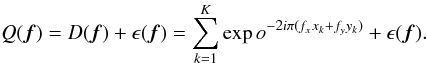 (A.3)Note that this
formalism is also valid for a temporal coding of the interferogram, which is replacing
the spatial position
(xk,yk)
by the (1-D) temporal sampling t, and similarly the spatial frequency
f by the temporal one ν.
(A.3)Note that this
formalism is also valid for a temporal coding of the interferogram, which is replacing
the spatial position
(xk,yk)
by the (1-D) temporal sampling t, and similarly the spatial frequency
f by the temporal one ν.
As Q represents the spectrum of the interferogram, the phase of the spectrum is merely
the argument of this estimator:
 (A.4)In this
framework, Chelli (1989) has shown that in first
approximation (i.e. small noise error), the variance of the phase can be expressed as
(A.4)In this
framework, Chelli (1989) has shown that in first
approximation (i.e. small noise error), the variance of the phase can be expressed as
![Mathematical equation: \appendix \setcounter{section}{1} \begin{equation} \sigma^2_{\phi} = \frac{1}{2}\frac{{E}(|Q|^2)-\mathrm{Re}[{E}(Q^2)]}{[{E}(Q)]^2}, \end{equation}](/articles/aa/full_html/2010/16/aa13356-09/aa13356-09-eq188.png) (A.5)then using Goodman’s
formalism described above, one can show that (Chelli
1989; Tatulli et al. 2004)
(A.5)then using Goodman’s
formalism described above, one can show that (Chelli
1989; Tatulli et al. 2004)
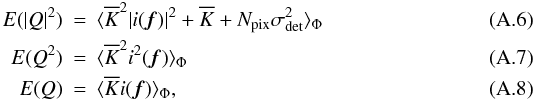 where
where
 is the average number of
photoevents per time unit, σdet is the detector noise and
Npix is the number of pixel to sample the signal.
i(f) is the normalized spectrum of the
interferogram (i.e. i(0) = 1).
is the average number of
photoevents per time unit, σdet is the detector noise and
Npix is the number of pixel to sample the signal.
i(f) is the normalized spectrum of the
interferogram (i.e. i(0) = 1).
⟨ ⟩ Φ denotes the expected value with respect to the atmosphere. How the previous expressions are unfolding depends on whether we deal with multimode or singlemode interferometry.
A.2. Useful definitions
In this section we introduce the concepts and notations that we will use in our formalism to derive the expression of the noise of the interferometric phase. Let us consider (see also Fig. 1 in the paper)
-
an interferometer made of two telescopes described by their pupil functions P1(r), P2(r) and their associated transmission
 ,
,
 .
Note that with this a definition P1 and
P2 are centered respectively at the position
r1 = λf1
and
r2 = λf2,
and we introduce the quantity
f12 = f2 − f1
as the baseline frequency of the interferometer.
.
Note that with this a definition P1 and
P2 are centered respectively at the position
r1 = λf1
and
r2 = λf2,
and we introduce the quantity
f12 = f2 − f1
as the baseline frequency of the interferometer. -
 and
and  the partially AO-corrected atmospheric
turbulent phase screens. We also introduce
the partially AO-corrected atmospheric
turbulent phase screens. We also introduce  the structure
function of the residual phases (assuming the same level of AO correction for each
telescope) together with
the structure
function of the residual phases (assuming the same level of AO correction for each
telescope) together with  ,
its associated residual phase variance (see also Appendix D).
,
its associated residual phase variance (see also Appendix D). -
the incoming wavefront of the source Ψ(r). By definition we have |Ψ(0)| 2 = N, where N is the number of photons per surface unit and per time unit emitted by the source, and [Ψ(r)Ψ ∗ (r + λf)] /|Ψ(0)| 2 = V(f) the visibility of the source at the spatial frequency f.
We emphasize that the following derivations will be done assuming monochromatic
interferograms at the wavelength λ. Indeed, taking into account a
non-null spectral bandwidth δλ is equivalent to considering a
monochromatic interferogram at the effective wavelength λ0
of the filter, modulated in amplitude by an envelope, whose width is fixed by the
spectral coherence length  . Moreover, this
effect is independent of the multimode or singlemode nature of the interferogram.
. Moreover, this
effect is independent of the multimode or singlemode nature of the interferogram.
A.3. Phase noise in multimode interferometry
Below we derive the estimator of the coherent flux of the interferogram, and subsequently the error of the interferometric phase in the multimode case. We provide two formalisms that respectively describe both beam recombination schemes: in the image plane and in the pupil plane.
A.3.1. Image plane recombination
Image plane recombination is well suited to describe multiaxial interferometric schemes where the fringe pattern is spatially coded on the detector, such as for the GI2T and VEGA/CHARA instruments. Note that co-axial (i.e. temporal) coding can also be performed in the image plane, but in practice – to our knowledge – no interferometric instruments are using this technique.
In this case, the spatial distribution of the complex amplitude of the radiation
field E(r) can be written as
 (A.9)By rules of
diffraction theory, the Fourier Transform of the interference pattern formed in the
image plane is the autocorrelation of the complex amplitude
E(r), namely
(A.9)By rules of
diffraction theory, the Fourier Transform of the interference pattern formed in the
image plane is the autocorrelation of the complex amplitude
E(r), namely
 (A.10)Introducing
| Ψ(0) | 2 = N in the above
equation enables us to make the complex visibility function appear:
(A.10)Introducing
| Ψ(0) | 2 = N in the above
equation enables us to make the complex visibility function appear:  (A.11)with
S1(f) and
S2(f) the so-called
photometric peaks resulting from the autocorrelation of each corrugated pupil, and
S12(f) the interferometric
peak arising from the cross-correlation between both pupils:
(A.11)with
S1(f) and
S2(f) the so-called
photometric peaks resulting from the autocorrelation of each corrugated pupil, and
S12(f) the interferometric
peak arising from the cross-correlation between both pupils:
![Mathematical equation: \appendix \setcounter{section}{1} \begin{eqnarray} S_{i}(f) = \int P_i({\vec r})P_i({\vec r}+\lambda{\vec f})\exp^{i(\phi^r_i({\vec r})-\phi^r_i({\vec r}+\lambda{\vec f}))}\mathrm{d}{\vec r},\quad {(i=[1,2])} \end{eqnarray}](/articles/aa/full_html/2010/16/aa13356-09/aa13356-09-eq224.png) (A.12)
(A.12)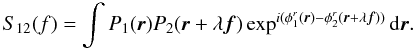 (A.13)From
Eq. (A.11), we can straightforwardly
derive the number of photoevents:
(A.13)From
Eq. (A.11), we can straightforwardly
derive the number of photoevents:  (A.14)which is
turbulence-independent (neglecting scintillation). ΣP is
the collecting area of a single telescope:
(A.14)which is
turbulence-independent (neglecting scintillation). ΣP is
the collecting area of a single telescope:
![Mathematical equation: \appendix \setcounter{section}{1} \begin{equation} \Sigma_P = \int [P_1({\vec r})]^2 \mathrm{d}{\vec r} = \int [P_2({\vec r})]^2 \mathrm{d}{\vec r}, \end{equation}](/articles/aa/full_html/2010/16/aa13356-09/aa13356-09-eq228.png) (A.15)assuming for the
sake of simplicity that both pupils are identical.
(A.15)assuming for the
sake of simplicity that both pupils are identical.
Equation (A.11) also shows that
multimode interferometry with image plane recombination continuously transmits the
whole spatial frequencies f. The complex visibility
V12 = V(f12)
is then derived from the estimate of the coherent flux at the baseline frequency of
the interferometer  , that is
 (A.16)and the normalized
spectrum of the interferogram takes the form
(A.16)and the normalized
spectrum of the interferogram takes the form 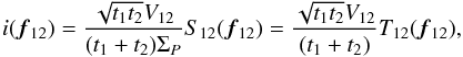 (A.17)where
T12(f) = S12(f)/ΣP
is the normalized interferometric transfer function, such as
|T12(f12) | = 1.
As a consequence, by analogy with the definition of the Strehl ratio for a single
telescope,
|T12(f12) | 2
can be seen as the instantaneous multimode interferometric Strehl
ratio.
(A.17)where
T12(f) = S12(f)/ΣP
is the normalized interferometric transfer function, such as
|T12(f12) | = 1.
As a consequence, by analogy with the definition of the Strehl ratio for a single
telescope,
|T12(f12) | 2
can be seen as the instantaneous multimode interferometric Strehl
ratio.
A.3.2. Pupil plane recombination
In this scheme, fringes are formed in the pupil plane by means of geometrical
operations of the entrance pupil (Chelli &
Mariotti 1986). This formalism is usually well suited to describe co-axial
recombination with temporal coding where the pupils are superimposed at the beam
splitter, hence the fringes formed in the pupil plane, as in the IOTA instrument. In
practice, the fringes are form by translating one pupil over the other (translation of
vector ), and by
introducing an optical path delay (θ1(t)
and θ2(t)) on each beam (see e.g. Buscher 1988, Appendix A2) to modulate the fringe
pattern. In this case, the complex amplitude of the superimposed electric fields
writes  (A.18)The fringe pattern
I(t) is then formed by focusing the light on one
single pixel of the detector. Again, by rules of image formation, it writes as
(A.18)The fringe pattern
I(t) is then formed by focusing the light on one
single pixel of the detector. Again, by rules of image formation, it writes as
 (A.19)which, by making
use of the expression of E(r)
rewrites as
(A.19)which, by making
use of the expression of E(r)
rewrites as
 (A.20)where
Δ12θ(t) = θ1(t) − θ2(t)
is the phase delay between the two beams that sample the fringe pattern. In the
Fourier plane, the interferometric equation takes the form
(A.20)where
Δ12θ(t) = θ1(t) − θ2(t)
is the phase delay between the two beams that sample the fringe pattern. In the
Fourier plane, the interferometric equation takes the form
 (A.21)where
δν is the Dirac function, and
ν12 is the temporal frequency at which the interferogram
is modulated, that is the frequency of the moving piezoelectric mirror.
(A.21)where
δν is the Dirac function, and
ν12 is the temporal frequency at which the interferogram
is modulated, that is the frequency of the moving piezoelectric mirror.
Note that at the difference of the image plane recombination, pupil plane
interferometry transmits only the frequency baseline . Nonetheless,
the coherent flux, estimated in the Fourier plane at the frequency mirror
(ν = ν12) takes the same form as in the
image plane case, namely:  (A.22)and similarly the
total number of detected photoevents is
(A.22)and similarly the
total number of detected photoevents is
 (A.23)and the normalized
spectrum of the interferogram at the frequency ν12 is
(A.23)and the normalized
spectrum of the interferogram at the frequency ν12 is
 (A.24)
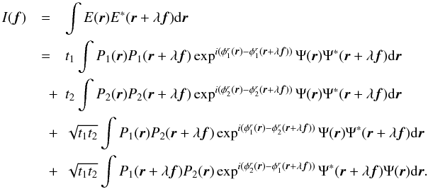
A.3.3. The interferometric phase error
In the above sections, we showed that independently of the chosen recombination
scheme, the total flux, the coherent flux, and consequently the normalized spectrum of
the interferogram can take the form of Eqs. (A.14–A.17), respectively.
Using these expressions, Eqs. (A.6–A.8) can be rewritten as
 (A.25)
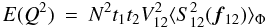 (A.26)
 (A.27)NB: Chelli
(1989) has shown that the error of the
phase does not depend on the object phase, hence one can consider in the following
that the object is centro-symmetric, that is
V12 = |V12| = Re [ V12 ] .
What remains now is to derive from the above equations the moments of the
interferometric transfer function
S12(f12):
(A.27)NB: Chelli
(1989) has shown that the error of the
phase does not depend on the object phase, hence one can consider in the following
that the object is centro-symmetric, that is
V12 = |V12| = Re [ V12 ] .
What remains now is to derive from the above equations the moments of the
interferometric transfer function
S12(f12):
 (A.28)
![Mathematical equation: \appendix \setcounter{section}{1} \begin{eqnarray} \langle S^2_{12}({\vec f_{12}})\rangle _{\Phi} &=& \int P_1({\vec r})P_2({\vec r}+\lambda{{\vec f_{12}}})P_1({\vec r}^{\prime})P_2({\vec r}^{\prime}+\lambda{{\vec f_{12}}})\langle \exp^{i(\phi^r_1({\vec r})-\phi^r_2({\vec r}+\lambda{{\vec f_{12}}})+\phi^r_1({\vec r}^{\prime})-\phi^r_2({\vec r}^{\prime}+\lambda{{\vec f_{12}}}))}\rangle _{\Phi}\mathrm{d}{\vec r}\mathrm{d}{{\vec r^{\prime}}}\nonumber \\ &=& P_1({\vec r})P_2({\vec r}+\lambda{{\vec f_{12}}})P_1({\vec r}^{\prime})P_2({\vec r}^{\prime}+\lambda{{\vec f_{12}}})\exp^{-\frac{1}{2}\langle |(\phi^r_1({\vec r})-\phi^r_2({\vec r}+\lambda{{\vec f_{12}}})+\phi^r_1({\vec r}^{\prime})-\phi^r_2({\vec r}^{\prime}+\lambda{{\vec f_{12}}}))|^2\rangle _{\Phi}}\mathrm{d}{\vec r}\mathrm{d}{{\vec r^{\prime}}} \nonumber \\ && \mbox{knowing that}~\langle \phi^r_1({\vec r})\phi^r_1({\vec r}^{\prime})\rangle _{\Phi} = \sigma^2_{\phi_r} - \frac{1}{2}\mathcal{D}_{\phi_r}({\vec r},{\vec r^{\prime}}),~\mbox{it comes}, \nonumber \\ &=& \exp^{-4\sigma^2_{\phi_r}} \int P_1({\vec r})P_2({\vec r}+\lambda{{\vec f_{12}}})P_1({\vec r}^{\prime})P_2({\vec r}^{\prime}+\lambda{{\vec f_{12}}})\exp^{\frac{1}{2}\mathcal{D}_{\phi_r}({\vec r},{\vec r^{\prime}})+\frac{1}{2}\mathcal{D}_{\phi_r}({\vec r}+\lambda{{\vec f_{12}}},{\vec r^{\prime}}+\lambda{{\vec f_{12}}})}\mathrm{d}{\vec r}\mathrm{d}{{\vec r^{\prime}}} \nonumber \\ && \mbox{changing axes reference:}~P_1({\vec r}),~P_2({\vec r})~\rightarrow~P({\vec r})~\mbox{centered on 0},\nonumber \\ \label{eq_i2_multi}&=& \exp^{-4\sigma^2_{\phi_r}} \int \left[ P({\vec r})P({\vec r}^{\prime})\exp^{\frac{1}{2}\mathcal{D}_{\phi_r}({\vec r},{\vec r^{\prime}})}\right]\left[P({\vec r})P({\vec r}^{\prime})\exp^{\frac{1}{2}\mathcal{D}_{\phi_r}({\vec r},{\vec r^{\prime}})}\right]\mathrm{d}{\vec r}\mathrm{d}{{\vec r^{\prime}}} \end{eqnarray}](/articles/aa/full_html/2010/16/aa13356-09/aa13356-09-eq256.png) (A.29)
(A.29)![Mathematical equation: \appendix \setcounter{section}{1} \begin{eqnarray} \langle |S_{12}({\vec f_{12}})|^2\rangle _{\Phi} &=& \int P_1({\vec r})P_2({\vec r}+\lambda{{\vec f_{12}}})P_1({\vec r}^{\prime})P_2({\vec r}^{\prime}+\lambda{{\vec f_{12}}})\langle \exp^{i(\phi^r_1({\vec r})-\phi^r_2({\vec r}+\lambda{{\vec f_{12}}})-\phi^r_1({\vec r}^{\prime})+\phi^r_2({\vec r}^{\prime}+\lambda{{\vec f_{12}}}))}\rangle _{\Phi}\mathrm{d}{\vec r}\mathrm{d}{{\vec r^{\prime}}} \nonumber \\ &=& \int P_1({\vec r})P_2({\vec r}+\lambda{{\vec f_{12}}})P_1({\vec r}^{\prime})P_2({\vec r}^{\prime}+\lambda{{\vec f_{12}}})\exp^{-\frac{1}{2}\langle |(\phi^r_1({\vec r})-\phi^r_2({\vec r}+\lambda{{\vec f_{12}}})-\phi^r_1({\vec r}^{\prime})+\phi^r_2({\vec r}^{\prime}+\lambda{{\vec f_{12}}}))|^2\rangle _{\Phi}}\mathrm{d}{\vec r}\mathrm{d}{{\vec r^{\prime}}} \nonumber \\ &=& \int P_1({\vec r})P_2({\vec r}+\lambda{{\vec f_{12}}})P_1({\vec r}^{\prime})P_2({\vec r}^{\prime}+\lambda{{\vec f_{12}}})\exp^{-\frac{1}{2}\mathcal{D}_{\phi_r}({\vec r},{\vec r^{\prime}})-\frac{1}{2}\mathcal{D}_{\phi_r}({\vec r}+\lambda{{\vec f_{12}}},{\vec r^{\prime}}+\lambda{{\vec f_{12}}})}\mathrm{d}{\vec r}\mathrm{d}{{\vec r^{\prime}}}\nonumber \\ && \mbox{changing axes reference:} \nonumber \\ \label{eq_absi2_multi}&=& \int \left[ P({\vec r})P({\vec r}^{\prime})\exp^{-\frac{1}{2}\mathcal{D}_{\phi_r}({\vec r},{\vec r^{\prime}})}\right]\left[P({\vec r})P({\vec r}^{\prime})\exp^{-\frac{1}{2}\mathcal{D}_{\phi_r}({\vec r},{\vec r^{\prime}})}\right]\mathrm{d}{\vec r}\mathrm{d}{{\vec r^{\prime}}}. \end{eqnarray}](/articles/aa/full_html/2010/16/aa13356-09/aa13356-09-eq257.png) (A.30)Putting
Eqs. (A.28, A.29, A.30) into Eqs. (A.25, A.26, A.27), we finally find that the variance
of the phase can be written as the quadratic sum of three terms, corresponding to the
detector, photon, and atmospheric regimes
(A.30)Putting
Eqs. (A.28, A.29, A.30) into Eqs. (A.25, A.26, A.27), we finally find that the variance
of the phase can be written as the quadratic sum of three terms, corresponding to the
detector, photon, and atmospheric regimes  respectively, with
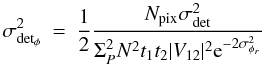 (A.31)
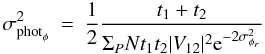 (A.32)
![Mathematical equation: \appendix \setcounter{section}{1} \begin{eqnarray} \sigma^2_{{\rm atm}_{\phi}}&=&\frac{1}{2}\frac{\int \left[P({\vec r})P({\vec r}^{\prime})\mathrm{e}^{-\frac{1}{2}\mathcal{D}_{\phi_r}({\vec r},{\vec r^{\prime}})}\right]^2\mathrm{d}{\vec r}\mathrm{d}{{\vec r^{\prime}}}-\mathrm{e}^{-4\sigma^2_{\phi_r}}\int \left[P({\vec r})P({\vec r}^{\prime})\mathrm{e}^{\frac{1}{2}\mathcal{D}_{\phi_r}({\vec r},{\vec r^{\prime}})}\right]^2\mathrm{d}{\vec r}\mathrm{d}{{\vec r^{\prime}}}}{\left[\int P^2({\vec r})\mathrm{d}{\vec r}\right]^2\mathrm{e}^{-2\sigma^2_{\phi_r}}}. \end{eqnarray}](/articles/aa/full_html/2010/16/aa13356-09/aa13356-09-eq261.png) (A.33)We
note that the expression of the variance for the photon noise
(
(A.33)We
note that the expression of the variance for the photon noise
( ) is the generalization
of the formula found by Vannier et al. (2006)
(Eq. (14)), when the visibility is corrupted by the partially AO-corrected turbulent
phase.
) is the generalization
of the formula found by Vannier et al. (2006)
(Eq. (14)), when the visibility is corrupted by the partially AO-corrected turbulent
phase.
A.4. Phase noise in singlemode interferometry
Because of the spatial filtering specific properties of singlemode devices, the
singlemode interferometric equation changes slightly with respect to that of the
multimode, because we have to take into account the coupling efficiency that extenuates
the number of coherent and incoherent photoevents. The coupling coefficients, for the
photometric (ρ1(V),
ρ2(V)), and interferometric
(ρ12(V)) channels respectively write
(Mège et al. 2003; Tatulli et al. 2004) ![Mathematical equation: \appendix \setcounter{section}{1} \begin{eqnarray} \rho_i(V)&=&\rho_0\frac{(V \ast S_{i})(\vec{0})}{\int S^0_i({\vec f})\mathrm{d}{\vec f}},~~ {(i=[1,2])} \nonumber \\ \label{app_eq_rhoi}&=& \rho_0\frac{\int V(f) P_i({\vec r})P_i({\vec r}+\lambda{\vec f})\exp^{i(\phi^r_i({\vec r})-\phi^r_i({\vec r}+\lambda{\vec f}))}\mathrm{d}{\vec r}\mathrm{d}{\vec f}}{\left[\int P_i({\vec r})\mathrm{d}{\vec r}\right]^2} \end{eqnarray}](/articles/aa/full_html/2010/16/aa13356-09/aa13356-09-eq266.png) (A.34)
(A.34)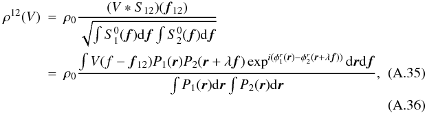 where
where
 ,
,  are the photometric transfer functions of a
perfect (atmosphere-free) interferometer, and ρ0 the maximum
coupling efficiency, shown to be ~80% (Shaklan
& Roddier 1988). And the singlemode interferometric equation writes:
are the photometric transfer functions of a
perfect (atmosphere-free) interferometer, and ρ0 the maximum
coupling efficiency, shown to be ~80% (Shaklan
& Roddier 1988). And the singlemode interferometric equation writes:
 (A.37)where
H1(f),
H2(f) and
H12(f) are the normalized
(i.e.
H1(0) = H2(0) = 1,
and H12(f12) = 1)
singlemode photometric and interferometric transfer functions, the so-called
carrying wave (Mège 2002),
which are fixed by the geometry of the singlemode device and therefore independent of
the atmosphere. As a result, the singlemode coherent flux is defined by
(A.37)where
H1(f),
H2(f) and
H12(f) are the normalized
(i.e.
H1(0) = H2(0) = 1,
and H12(f12) = 1)
singlemode photometric and interferometric transfer functions, the so-called
carrying wave (Mège 2002),
which are fixed by the geometry of the singlemode device and therefore independent of
the atmosphere. As a result, the singlemode coherent flux is defined by 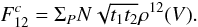 (A.38)
A.4.1. Compact sources case
For compact sources – which are those unresolved by the telescope, which is the most
common case in interferometry – Eqs. (A.34) and (A.35) are taking
the simplified following form:
![Mathematical equation: \appendix \setcounter{section}{1} \begin{eqnarray} \rho_i(V)&=& \rho_0\frac{\int P_i({\vec r})P_i({\vec r}+\lambda{\vec f})\exp^{i(\phi^r_i({\vec r})-\phi^r_i({\vec r}+\lambda{\vec f}))}\mathrm{d}{\vec r}\mathrm{d}{\vec f}}{\left[\int P_i({\vec r})\mathrm{d}{\vec r}\right]^2} = \rho_0 \mathcal{S}_i \end{eqnarray}](/articles/aa/full_html/2010/16/aa13356-09/aa13356-09-eq280.png) (A.39)
(A.39)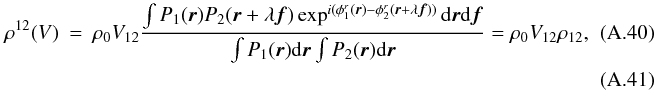 where
where
 is by
definition the instantaneous Strehl ratio relative to the ith
telescope, and with
is by
definition the instantaneous Strehl ratio relative to the ith
telescope, and with 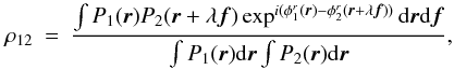 (A.42) |ρ12| 2
being by analogy the instantaneous singlemode interferometric Strehl
ratio. The interferometric equation finally rewrites
(A.42) |ρ12| 2
being by analogy the instantaneous singlemode interferometric Strehl
ratio. The interferometric equation finally rewrites
 (A.43)And the singlemode
coherent flux at the spatial frequency takes the form:
(A.43)And the singlemode
coherent flux at the spatial frequency takes the form:
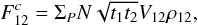 (A.44)whereas the number of
photoevents writes
(A.44)whereas the number of
photoevents writes  (A.45)which depends on
the turbulent atmosphere through the fluctuations of the instantaneous Strehl ratio
(A.45)which depends on
the turbulent atmosphere through the fluctuations of the instantaneous Strehl ratio
 and
and
 . And
the normalized spectrum of the interferogram is
. And
the normalized spectrum of the interferogram is
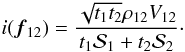 (A.46)The generic equations
of the phase noise thus rewrites
(A.46)The generic equations
of the phase noise thus rewrites  (A.47)
 (A.48)
 (A.49)Now
we need to compute the moments of the coupling coefficients:
(A.49)Now
we need to compute the moments of the coupling coefficients: ![Mathematical equation: \appendix \setcounter{section}{1} \begin{eqnarray} \label{eq_rho_mono}\langle \mathcal{S}_i\rangle _{\Phi} &=& \overline{\mathcal{S}_i},~~\mbox{(i=[1,2])}, \end{eqnarray}](/articles/aa/full_html/2010/16/aa13356-09/aa13356-09-eq295.png) (A.50)where
(A.50)where
 is the long
exposure Strehl ratio of the ith telescope. Assuming equivalent AO
correction for both telescopes, we have
is the long
exposure Strehl ratio of the ith telescope. Assuming equivalent AO
correction for both telescopes, we have 
 (A.51)which
shows that the long exposure interferometric Strehl ratio is equal to
the coherent energy
(A.51)which
shows that the long exposure interferometric Strehl ratio is equal to
the coherent energy  .
.
![Mathematical equation: \appendix \setcounter{section}{1} \begin{eqnarray} \langle \rho_{12}^2\rangle _{\Phi}&=&\frac{\int P_1({\vec r})P_2({\vec r}+\lambda{\vec f})P_1({\vec r}^{\prime})P_2({\vec r}^{\prime}+\lambda{{\vec f^{\prime}}})\langle \exp^{i(\phi^r_1({\vec r})+\phi^r_1({\vec r}^{\prime})-\phi^r_2({\vec r}+\lambda{\vec f})-\phi^r_2({\vec r}^{\prime}+\lambda{{\vec f^{\prime}}}))}\rangle _{\Phi}\mathrm{d}{\vec r}\mathrm{d}{\vec r^{\prime}}\mathrm{d}{\vec f}\mathrm{d}{\vec f}^{\prime}}{\left[\int P_1({\vec r})\mathrm{d}{\vec r} \int P_2({\vec r})\mathrm{d}{\vec r}\right]^2}\nonumber\\ &=&\mathrm{e}^{-4\sigma^2_{\phi_r}}\frac{\int P_1({\vec r})P_2({\vec r}+\lambda{\vec f})P_1({\vec r}^{\prime})P_2({\vec r}^{\prime}+\lambda{{\vec f^{\prime}}})\exp^{\frac{1}{2}\mathcal{D}_{\phi_r}({\vec r},{\vec r^{\prime}})+\frac{1}{2}\mathcal{D}_{\phi_r}({\vec r}+\lambda{\vec f},{\vec r^{\prime}}+\lambda{{\vec f^{\prime}}})}\mathrm{d}{\vec r}\mathrm{d}{\vec r^{\prime}}\mathrm{d}{\vec f}\mathrm{d}{\vec f}^{\prime}}{\left[\int P_1({\vec r})\mathrm{d}{\vec r} \int P_2({\vec r})\mathrm{d}{\vec r}\right]^2}\nonumber\\ && \mbox{change of variables}~{\vec r}+\lambda{\vec f} \rightarrow {\vec u}, {\vec r^{\prime}}+\lambda{{\vec f^{\prime}}} \rightarrow {\vec u^{\prime}}:\nonumber\\ \label{eq_rhoij2_mono}&=&\mathrm{e}^{-4\sigma^2_{\phi_r}}\frac{\int P_1({\vec r})P_1({\vec r}^{\prime})\exp^{\frac{1}{2}\mathcal{D}_{\phi_r}({\vec r},{\vec r^{\prime}})}\mathrm{d}{\vec r}\mathrm{d}{\vec r^{\prime}}\int P_2({\vec r})P_2({\vec r}^{\prime})\exp^{\frac{1}{2}\mathcal{D}_{\phi_r}({\vec r},{\vec r^{\prime}})}\mathrm{d}{\vec r}\mathrm{d}{\vec r^{\prime}}}{\left[\int P_1({\vec r})\mathrm{d}{\vec r} \int P_2({\vec r})\mathrm{d}{\vec r}\right]^2} \end{eqnarray}](/articles/aa/full_html/2010/16/aa13356-09/aa13356-09-eq300.png) (A.52)
(A.52)![Mathematical equation: \appendix \setcounter{section}{1} \begin{eqnarray} \langle |\rho_{12}|^2\rangle _{\Phi}&=&\frac{\int P_1({\vec r})P_2({\vec r}+\lambda{\vec f})P_1({\vec r}^{\prime})P_2({\vec r}^{\prime}+\lambda{{\vec f^{\prime}}})\langle \exp^{i(\phi^r_1({\vec r})-\phi^r_1({\vec r}^{\prime})-\phi^r_2({\vec r}+\lambda{\vec f})+\phi^r_2({\vec r}^{\prime}+\lambda{{\vec f^{\prime}}}))}\rangle _{\Phi}\mathrm{d}{\vec r}\mathrm{d}{\vec r^{\prime}}\mathrm{d}{\vec f}\mathrm{d}{\vec f}^{\prime}}{\left[\int P_1({\vec r})\mathrm{d}{\vec r} \int P_2({\vec r})\mathrm{d}{\vec r}\right]^2}\nonumber\\ &=&\frac{\int P_1({\vec r})P_2({\vec r}+\lambda{\vec f})P_1({\vec r}^{\prime})P_2({\vec r}^{\prime}+\lambda{{\vec f^{\prime}}})\exp^{-\frac{1}{2}\mathcal{D}_{\phi_r}({\vec r},{\vec r^{\prime}})-\frac{1}{2}\mathcal{D}_{\phi_r}({\vec r}+\lambda{\vec f},{\vec r^{\prime}}+\lambda{{\vec f^{\prime}}})}\mathrm{d}{\vec r}\mathrm{d}{\vec r^{\prime}}\mathrm{d}{\vec f}\mathrm{d}{\vec f}^{\prime}}{\left[\int P_1({\vec r})\mathrm{d}{\vec r} \int P_2({\vec r})\mathrm{d}{\vec r}\right]^2}\nonumber\\ && \mbox{change of variables}~{\vec r}+\lambda{\vec f} \rightarrow {\vec u}, {\vec r^{\prime}}+\lambda{{\vec f^{\prime}}} \rightarrow {\vec u^{\prime}}:\nonumber\\ \label{eq_absrhoij2_mono}&=&\frac{\int P_1({\vec r})P_1({\vec r}^{\prime})\exp^{-\frac{1}{2}\mathcal{D}_{\phi_r}({\vec r},{\vec r^{\prime}})}\mathrm{d}{\vec r}\mathrm{d}{\vec r^{\prime}}\int P_2({\vec r})P_2({\vec r}^{\prime})\exp^{-\frac{1}{2}\mathcal{D}_{\phi_r}({\vec r},{\vec r^{\prime}})}\mathrm{d}{\vec r}\mathrm{d}{\vec r^{\prime}}}{\left[\int P_1({\vec r})\mathrm{d}{\vec r} \int P_2({\vec r})\mathrm{d}{\vec r}\right]^2}\cdot \end{eqnarray}](/articles/aa/full_html/2010/16/aa13356-09/aa13356-09-eq301.png) (A.53)Putting
Eqs. (A.50, A.51, A.52, A.53) into
Eqs. (A.47, A.48, A.49), we find again that the variance of the phase can be written
as the quadratic sum of three terms, corresponding to the detector, photon, and
atmospheric regimes respectively, with
(A.53)Putting
Eqs. (A.50, A.51, A.52, A.53) into
Eqs. (A.47, A.48, A.49), we find again that the variance of the phase can be written
as the quadratic sum of three terms, corresponding to the detector, photon, and
atmospheric regimes respectively, with
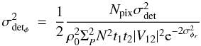 (A.54)
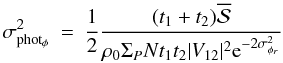 (A.55)
![Mathematical equation: \appendix \setcounter{section}{1} \begin{eqnarray} \sigma^2_{{\rm atm}_{\phi}}&=&\frac{1}{2}\frac{\left[\int P({\vec r})P({\vec r}^{\prime})\mathrm{e}^{-\frac{1}{2}\mathcal{D}_{\phi_r}({\vec r},{\vec r^{\prime}})}\mathrm{d}{\vec r}\mathrm{d}{{\vec r^{\prime}}}\right]^2-\mathrm{e}^{-4\sigma^2_{\phi_r}}\left[\int P({\vec r})P({\vec r}^{\prime})\mathrm{e}^{\frac{1}{2}\mathcal{D}_{\phi_r}({\vec r},{\vec r^{\prime}})}\mathrm{d}{\vec r}\mathrm{d}{{\vec r^{\prime}}}\right]^2}{\left[\int P({\vec r})\mathrm{d}{\vec r}\right]^4\mathrm{e}^{-2\sigma^2_{\phi_r}}}\cdot \end{eqnarray}](/articles/aa/full_html/2010/16/aa13356-09/aa13356-09-eq304.png) (A.56)
(A.56)
Appendix B: Coherent flux dropouts - Rician density probability
By analogy with the study of Canales & Cagigal
(1999) on the statistics of the instantaneous Strehl ratio in partial AO
correction, the instantaneous interferometric Strehl ratio, namely
I = |T12| 2 and
I = |ρ12| 2 for multimode and
singlemode interferometers respectively are shown to follow Rician density probability
statistics of the form:  (B.1)In this appendix, we aim
to derive the theoretical expression of the moments of the Rician distribution (namely
a and σ), in both multimode and singlemode cases.
Following Canales & Cagigal (1999), the
quantity a and σ can be expressed from the moments of
the real (Ar) and imaginary
(Ai) parts of the complex instantaneous
interferometric Strehl ratio (i.e. such as
(B.1)In this appendix, we aim
to derive the theoretical expression of the moments of the Rician distribution (namely
a and σ), in both multimode and singlemode cases.
Following Canales & Cagigal (1999), the
quantity a and σ can be expressed from the moments of
the real (Ar) and imaginary
(Ai) parts of the complex instantaneous
interferometric Strehl ratio (i.e. such as  ):
):  where
where
 and
and 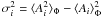 .
.
B.1. Multimode case
In multimode interferometry we have
I = |T12| 2, hence
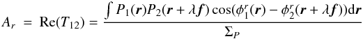 (B.4)
(B.4)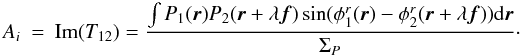 (B.5)Following
the same approach as in appendix A.3, we compute
the first and second order moments of these quantities.
(B.5)Following
the same approach as in appendix A.3, we compute
the first and second order moments of these quantities.  (B.6)
(B.6) (B.7)
(B.7)![Mathematical equation: \appendix \setcounter{section}{2} \begin{eqnarray} \langle A_r^2\rangle _{\Phi} &=& \frac{\int P_1({\vec r})P_2({\vec r}+\lambda{{\vec f_{12}}})P_1({\vec r}^{\prime})P_2({\vec r}^{\prime}+\lambda{{\vec f_{12}}})\langle \cos(\phi^r_1({\vec r})-\phi^r_2({\vec r}+\lambda{{\vec f_{12}}}))\cos(\phi^r_1({\vec r}^{\prime})-\phi^r_2({\vec r}^{\prime}+\lambda{{\vec f_{12}}}))\rangle _{\Phi}\mathrm{d}{\vec r}\mathrm{d}{{\vec r^{\prime}}}}{\Sigma_P^2} \nonumber \\ && \mbox{using}~\cos(a)\cos(b) = (\cos(a-b) + \cos(a+b))/2 \nonumber\\ &=& \frac{1}{2}\frac{\int P_1({\vec r})P_2({\vec r}+\lambda{{\vec f_{12}}})P_1({\vec r}^{\prime})P_2({\vec r}^{\prime}+\lambda{{\vec f_{12}}})\langle \cos(\phi^r_1({\vec r})-\phi^r_2({\vec r}+\lambda{{\vec f_{12}}})-\phi^r_1({\vec r}^{\prime})+\phi^r_2({\vec r}^{\prime}+\lambda{{\vec f_{12}}}))\rangle _{\Phi}\mathrm{d}{\vec r}\mathrm{d}{{\vec r^{\prime}}}}{\Sigma_P^2} \nonumber \\ && + \frac{1}{2}\frac{\int P_1({\vec r})P_2({\vec r}+\lambda{{\vec f_{12}}})P_1({\vec r}^{\prime})P_2({\vec r}^{\prime}+\lambda{{\vec f_{12}}})\langle \cos(\phi^r_1({\vec r})-\phi^r_2({\vec r}+\lambda{{\vec f_{12}}})+\phi^r_1({\vec r}^{\prime})-\phi^r_2({\vec r}^{\prime}+\lambda{{\vec f_{12}}}))\rangle _{\Phi}\mathrm{d}{\vec r}\mathrm{d}{{\vec r^{\prime}}}}{\Sigma_P^2} \nonumber \\ && \mbox{changing axes reference:}~P_1,~P_2~\mbox{centered on 0},\nonumber \\ &=& \frac{1}{2} \frac{\int \left[ P({\vec r})P({\vec r}^{\prime})\exp^{-\frac{1}{2}\mathcal{D}_{\phi_r}({\vec r},{\vec r^{\prime}})}\right]\left[P({\vec r})P({\vec r}^{\prime})\exp^{-\frac{1}{2}\mathcal{D}_{\phi_r}({\vec r},{\vec r^{\prime}})}\right]\mathrm{d}{\vec r}\mathrm{d}{{\vec r^{\prime}}}}{\left[\int P^2({\vec r})\mathrm{d}{\vec r}\right]^2} \nonumber \\ \label{eq_ar2_multi}&& + \frac{1}{2} \exp^{-4\sigma^2_{\phi_r}} \frac{\int \left[ P({\vec r})P({\vec r}^{\prime})\exp^{\frac{1}{2}\mathcal{D}_{\phi_r}({\vec r},{\vec r^{\prime}})}\right]\left[P({\vec r})P({\vec r}^{\prime})\exp^{\frac{1}{2}\mathcal{D}_{\phi_r}({\vec r},{\vec r^{\prime}})}\right]\mathrm{d}{\vec r}\mathrm{d}{{\vec r^{\prime}}}}{\left[\int P^2({\vec r})\mathrm{d}{\vec r}\right]^2} \end{eqnarray}](/articles/aa/full_html/2010/16/aa13356-09/aa13356-09-eq320.png) (B.8)
(B.8)![Mathematical equation: \appendix \setcounter{section}{2} \begin{eqnarray} \langle A_i^2\rangle _{\Phi} &=& \frac{\int P_1({\vec r})P_2({\vec r}+\lambda{{\vec f_{12}}})P_1({\vec r}^{\prime})P_2({\vec r}^{\prime}+\lambda{{\vec f_{12}}})\langle \sin(\phi^r_1({\vec r})-\phi^r_2({\vec r}+\lambda{{\vec f_{12}}}))\sin(\phi^r_1({\vec r}^{\prime})-\phi^r_2({\vec r}^{\prime}+\lambda{{\vec f_{12}}}))\rangle _{\Phi}\mathrm{d}{\vec r}\mathrm{d}{{\vec r^{\prime}}}}{\Sigma_P^2} \nonumber \\ && \mbox{using}~\sin(a)\sin(b) = (\cos(a-b) - \cos(a+b))/2 \nonumber\\ &=& \frac{1}{2}\frac{\int P_1({\vec r})P_2({\vec r}+\lambda{{\vec f_{12}}})P_1({\vec r}^{\prime})P_2({\vec r}^{\prime}+\lambda{{\vec f_{12}}})\langle \cos(\phi^r_1({\vec r})-\phi^r_2({\vec r}+\lambda{{\vec f_{12}}})-\phi^r_1({\vec r}^{\prime})+\phi^r_2({\vec r}^{\prime}+\lambda{{\vec f_{12}}}))\rangle _{\Phi}\mathrm{d}{\vec r}\mathrm{d}{{\vec r^{\prime}}}}{\Sigma_P^2} \nonumber \\ && - \frac{1}{2}\frac{\int P_1({\vec r})P_2({\vec r}+\lambda{{\vec f_{12}}})P_1({\vec r}^{\prime})P_2({\vec r}^{\prime}+\lambda{{\vec f_{12}}})\langle \cos(\phi^r_1({\vec r})-\phi^r_2({\vec r}+\lambda{{\vec f_{12}}})+\phi^r_1({\vec r}^{\prime})-\phi^r_2({\vec r}^{\prime}+\lambda{{\vec f_{12}}}))\rangle _{\Phi}\mathrm{d}{\vec r}\mathrm{d}{{\vec r^{\prime}}}}{\Sigma_P^2} \nonumber \\ && \mbox{changing axes reference:}~P_1,~P_2~\mbox{centered on 0},\nonumber \\ &=& \frac{1}{2} \frac{\int \left[ P({\vec r})P({\vec r}^{\prime})\exp^{-\frac{1}{2}\mathcal{D}_{\phi_r}({\vec r},{\vec r^{\prime}})}\right]\left[P({\vec r})P({\vec r}^{\prime})\exp^{-\frac{1}{2}\mathcal{D}_{\phi_r}({\vec r},{\vec r^{\prime}})}\right]\mathrm{d}{\vec r}\mathrm{d}{{\vec r^{\prime}}}}{\left[\int P^2({\vec r})\mathrm{d}{\vec r}\right]^2} \nonumber \\ \label{eq_ai2_multi}&& - \frac{1}{2} \exp^{-4\sigma^2_{\phi_r}} \frac{\int \left[ P({\vec r})P({\vec r}^{\prime})\exp^{\frac{1}{2}\mathcal{D}_{\phi_r}({\vec r},{\vec r^{\prime}})}\right]\left[P({\vec r})P({\vec r}^{\prime})\exp^{\frac{1}{2}\mathcal{D}_{\phi_r}({\vec r},{\vec r^{\prime}})}\right]\mathrm{d}{\vec r}\mathrm{d}{{\vec r^{\prime}}}}{\left[\int P^2({\vec r})\mathrm{d}{\vec r}\right]^2} \end{eqnarray}](/articles/aa/full_html/2010/16/aa13356-09/aa13356-09-eq321.png) (B.9)Using
Eqs. (B.6, B.7, B.8, B.9) in
Eqs. (B.2, B.3), we obtain the theoretical expressions
of the parameters a and σ of the Rician distribution
is the multimode case, as summarized in Table B.1
of the appendix.
(B.9)Using
Eqs. (B.6, B.7, B.8, B.9) in
Eqs. (B.2, B.3), we obtain the theoretical expressions
of the parameters a and σ of the Rician distribution
is the multimode case, as summarized in Table B.1
of the appendix.
Parameters a and σ of the Rician probability distribution function for both multimode and singlemode cases.
B.2. Singlemode case
In singlemode interferometry we have
I = |ρ12| 2, hence
 (B.10)
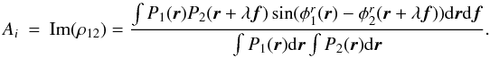 (B.11)Following
the same formalism as above, we compute the first and second order moments of these
quantities.
(B.11)Following
the same formalism as above, we compute the first and second order moments of these
quantities. 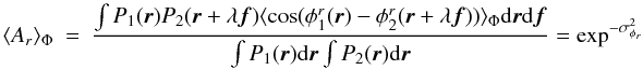 (B.12)
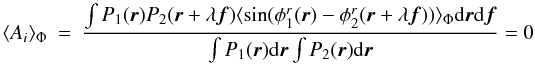 (B.13)
![Mathematical equation: \appendix \setcounter{section}{2} \begin{eqnarray} \langle A_r^2\rangle _{\Phi} &=& \frac{\int P_1({\vec r})P_2({\vec r}+\lambda{\vec f})P_1({\vec r}^{\prime})P_2({\vec r}^{\prime}+\lambda{{\vec f^{\prime}}})\langle \cos(\phi^r_1({\vec r})-\phi^r_2({\vec r}+\lambda{\vec f}))\cos(\phi^r_1({\vec r}^{\prime})-\phi^r_2({\vec r}^{\prime}+\lambda{{\vec f^{\prime}}}))\rangle _{\Phi}\mathrm{d}{\vec r}\mathrm{d}{\vec r^{\prime}}\mathrm{d}{\vec f}\mathrm{d}{\vec f}^{\prime}}{\left[\int P_1({\vec r})\mathrm{d}{\vec r} \int P_2({\vec r})\mathrm{d}{\vec r}\right]^2} \nonumber \\ && \mbox{using}~\cos(a)\cos(b) = (\cos(a-b) + \cos(a+b))/2 \nonumber\\ &=& \frac{1}{2}\frac{\int P_1({\vec r})P_2({\vec r}+\lambda{\vec f})P_1({\vec r}^{\prime})P_2({\vec r}^{\prime}+\lambda{{\vec f^{\prime}}})\langle \cos(\phi^r_1({\vec r})-\phi^r_2({\vec r}+\lambda{\vec f})-\phi^r_1({\vec r}^{\prime})+\phi^r_2({\vec r}^{\prime}+\lambda{{\vec f^{\prime}}})\rangle _{\Phi}\mathrm{d}{\vec r}\mathrm{d}{\vec r^{\prime}}\mathrm{d}{\vec f}\mathrm{d}{\vec f}^{\prime}}{\left[\int P_1({\vec r})\mathrm{d}{\vec r} \int P_2({\vec r})\mathrm{d}{\vec r}\right]^2} \nonumber\\ && + \frac{1}{2}\frac{\int P_1({\vec r})P_2({\vec r}+\lambda{\vec f})P_1({\vec r}^{\prime})P_2({\vec r}^{\prime}+\lambda{{\vec f^{\prime}}})\langle \cos(\phi^r_1({\vec r})-\phi^r_2({\vec r}+\lambda{\vec f})+\phi^r_1({\vec r}^{\prime})-\phi^r_2({\vec r}^{\prime}+\lambda{{\vec f^{\prime}}}))\rangle _{\Phi}\mathrm{d}{\vec r}\mathrm{d}{\vec r^{\prime}}\mathrm{d}{\vec f}\mathrm{d}{\vec f}^{\prime}}{\left[\int P_1({\vec r})\mathrm{d}{\vec r} \int P_2({\vec r})\mathrm{d}{\vec r}\right]^2} \nonumber \\ && \mbox{change of variables}~{\vec r}+\lambda{\vec f} \rightarrow u, {\vec r^{\prime}}+\lambda{{\vec f^{\prime}}} \rightarrow {\vec u^{\prime}}:\nonumber\\ &=&\frac{1}{2}\frac{\int P_1({\vec r})P_1({\vec r}^{\prime})\exp^{-\frac{1}{2}\mathcal{D}_{\phi_r}({\vec r},{\vec r^{\prime}})}\mathrm{d}{\vec r}\mathrm{d}{\vec r^{\prime}}\int P_2({\vec r})P_2({\vec r}^{\prime})\exp^{-\frac{1}{2}\mathcal{D}_{\phi_r}({\vec r},{\vec r^{\prime}})}\mathrm{d}{\vec r}\mathrm{d}{\vec r^{\prime}}}{\left[\int P_1({\vec r})\mathrm{d}{\vec r} \int P_2({\vec r})\mathrm{d}{\vec r}\right]^2} \nonumber\\ \label{eq_ar2_mono}&& + \mathrm{e}^{-4\sigma^2_{\phi_r}}\frac{\int P_1({\vec r})P_1({\vec r}^{\prime})\exp^{\frac{1}{2}\mathcal{D}_{\phi_r}({\vec r},{\vec r^{\prime}})}\mathrm{d}{\vec r}\mathrm{d}{\vec r^{\prime}}\int P_2({\vec r})P_2({\vec r}^{\prime})\exp^{\frac{1}{2}\mathcal{D}_{\phi_r}({\vec r},{\vec r^{\prime}})}\mathrm{d}{\vec r}\mathrm{d}{\vec r^{\prime}}}{\left[\int P_1({\vec r})\mathrm{d}{\vec r} \int P_2({\vec r})\mathrm{d}{\vec r}\right]^2} \end{eqnarray}](/articles/aa/full_html/2010/16/aa13356-09/aa13356-09-eq334.png) (B.14)
(B.14)![Mathematical equation: \appendix \setcounter{section}{2} \begin{eqnarray} \langle A_i^2\rangle _{\Phi} &=& \frac{\int P_1({\vec r})P_2({\vec r}+\lambda{\vec f})P_1({\vec r}^{\prime})P_2({\vec r}^{\prime}+\lambda{{\vec f^{\prime}}})\langle \sin(\phi^r_1({\vec r})-\phi^r_2({\vec r}+\lambda{\vec f}))\sin(\phi^r_1({\vec r}^{\prime})-\phi^r_2({\vec r}^{\prime}+\lambda{{\vec f^{\prime}}}))\rangle _{\Phi}\mathrm{d}{\vec r}\mathrm{d}{\vec r^{\prime}}\mathrm{d}{\vec f}\mathrm{d}{\vec f}^{\prime}}{\left[\int P_1({\vec r})\mathrm{d}{\vec r} \int P_2({\vec r})\mathrm{d}{\vec r}\right]^2} \nonumber \\ && \mbox{using}~\sin(a)\sin(b) = (\cos(a-b) - \cos(a+b))/2 \nonumber\\ &=& \frac{1}{2}\frac{\int P_1({\vec r})P_2({\vec r}+\lambda{\vec f})P_1({\vec r}^{\prime})P_2({\vec r}^{\prime}+\lambda{{\vec f^{\prime}}})\langle \cos(\phi^r_1({\vec r})-\phi^r_2({\vec r}+\lambda{\vec f})-\phi^r_1({\vec r}^{\prime})+\phi^r_2({\vec r}^{\prime}+\lambda{{\vec f^{\prime}}})\rangle _{\Phi}\mathrm{d}{\vec r}\mathrm{d}{\vec r^{\prime}}\mathrm{d}{\vec f}\mathrm{d}{\vec f}^{\prime}}{\left[\int P_1({\vec r})\mathrm{d}{\vec r} \int P_2({\vec r})\mathrm{d}{\vec r}\right]^2} \nonumber\\ && - \frac{1}{2}\frac{\int P_1({\vec r})P_2({\vec r}+\lambda{\vec f})P_1({\vec r}^{\prime})P_2({\vec r}^{\prime}+\lambda{{\vec f^{\prime}}})\langle \cos(\phi^r_1({\vec r})-\phi^r_2({\vec r}+\lambda{\vec f})+\phi^r_1({\vec r}^{\prime})-\phi^r_2({\vec r}^{\prime}+\lambda{{\vec f^{\prime}}})\rangle _{\Phi}\mathrm{d}{\vec r}\mathrm{d}{\vec r^{\prime}}\mathrm{d}{\vec f}\mathrm{d}{\vec f}^{\prime}}{\left[\int P_1({\vec r})\mathrm{d}{\vec r} \int P_2({\vec r})\mathrm{d}{\vec r}\right]^2} \nonumber \\ && \mbox{change of variables}~{\vec r}+\lambda{\vec f} \rightarrow {\vec u}, {\vec r^{\prime}}+\lambda{{\vec f^{\prime}}} \rightarrow {\vec u^{\prime}}:\nonumber\\ &=&\frac{1}{2}\frac{\int P_1({\vec r})P_1({\vec r}^{\prime})\exp^{-\frac{1}{2}\mathcal{D}_{\phi_r}({\vec r},{\vec r^{\prime}})}\mathrm{d}{\vec r}\mathrm{d}{\vec r^{\prime}}\int P_2({\vec r})P_2({\vec r}^{\prime})\exp^{-\frac{1}{2}\mathcal{D}_{\phi_r}({\vec r},{\vec r^{\prime}})}\mathrm{d}{\vec r}\mathrm{d}{\vec r^{\prime}}}{\left[\int P_1({\vec r})\mathrm{d}{\vec r} \int P_2({\vec r})\mathrm{d}{\vec r}\right]^2} \nonumber\\ \label{eq_ai2_mono}&& - \mathrm{e}^{-4\sigma^2_{\phi_r}}\frac{\int P_1({\vec r})P_1({\vec r}^{\prime})\exp^{\frac{1}{2}\mathcal{D}_{\phi_r}({\vec r},{\vec r^{\prime}})}\mathrm{d}{\vec r}\mathrm{d}{\vec r^{\prime}}\int P_2({\vec r})P_2({\vec r}^{\prime})\exp^{\frac{1}{2}\mathcal{D}_{\phi_r}({\vec r},{\vec r^{\prime}})}\mathrm{d}{\vec r}\mathrm{d}{\vec r^{\prime}}}{\left[\int P_1({\vec r})\mathrm{d}{\vec r} \int P_2({\vec r})\mathrm{d}{\vec r}\right]^2}. \end{eqnarray}](/articles/aa/full_html/2010/16/aa13356-09/aa13356-09-eq335.png) (B.15)Putting
Eqs. (B.12, B.13, B.14, B.15) in
Eqs. (B.2, B.3), we obtain the theoretical expressions
of the parameters a and σ of the Rician distribution
is the singlemode case, as summarized in Table B.1 of the appendix.
(B.15)Putting
Eqs. (B.12, B.13, B.14, B.15) in
Eqs. (B.2, B.3), we obtain the theoretical expressions
of the parameters a and σ of the Rician distribution
is the singlemode case, as summarized in Table B.1 of the appendix.
Appendix C: Astrometric phase error
The astrometric phase error writes  (C.1)where
φs, and
(C.1)where
φs, and  are the partially
AO-corrected phase of the astrophysical target and the phase estimated from the off-axis
reference source respectively. Δα
is the angular separation between both sources, and h is the altitude of the turbulent
layer. Since
are the partially
AO-corrected phase of the astrophysical target and the phase estimated from the off-axis
reference source respectively. Δα
is the angular separation between both sources, and h is the altitude of the turbulent
layer. Since  has been computed in previous
sections, we now need to compute the covariance part of Eq. (C.1). The formal expression of the covariance is given by Chelli (1989):
has been computed in previous
sections, we now need to compute the covariance part of Eq. (C.1). The formal expression of the covariance is given by Chelli (1989):
![Mathematical equation: \appendix \setcounter{section}{3} \begin{equation} \mathrm{cov}(\phi_s, \phi_r^{\Delta\alpha{h}}) = \frac{1}{2}\frac{\mathrm{Re}[{E}(QQ^{\ast}_{\Delta\alpha{h}})]-\mathrm{Re}[{E}(QQ_{\Delta\alpha{h}})]}{{E}(Q){E}(Q_{\Delta\alpha{h}})}, \end{equation}](/articles/aa/full_html/2010/16/aa13356-09/aa13356-09-eq341.png) (C.2)where
QΔαh is the estimator of the coherent
flux for the off-axis reference source.
(C.2)where
QΔαh is the estimator of the coherent
flux for the off-axis reference source.
C.1. Multimode case
Using the equations of Sect. A, one can derive
the moments of the multimode estimator:  (C.3)
(C.3) (C.4)
(C.4) (C.5)
(C.5) (C.6)where
NΔαh and
(C.6)where
NΔαh and  are the number of
photons (per surface unit and per time unit) and the visibility of the reference source
respectively, and with
are the number of
photons (per surface unit and per time unit) and the visibility of the reference source
respectively, and with  (C.7)Since
we assume one turbulent layer to be located at the altitude h, we have
by definition
(C.7)Since
we assume one turbulent layer to be located at the altitude h, we have
by definition  and
and
 , hence:
  (C.8)Furthermore,
we have
(C.8)Furthermore,
we have ![Mathematical equation: \appendix \setcounter{section}{3} \begin{eqnarray} && \langle S_{12}({\vec f_{12}})S^{\Delta\alpha{h}}_{12}({\vec f_{12}})\rangle _{\Phi} \nonumber \\ &&= \int P_1({\vec r})P_2({\vec r}+\lambda{{\vec f_{12}}})P_1({\vec r}^{\prime})P_2({\vec r}^{\prime}+\lambda{{\vec f_{12}}})\langle \exp^{i(\phi_1({\vec r})-\phi_2({\vec r}+\lambda{{\vec f_{12}}})+\phi_1({\vec r}^{\prime}+\vec{\Delta\alpha}{h})-\phi_2({\vec r}^{\prime}+\lambda{{\vec f_{12}}+\vec{\Delta\alpha}{h}}))}\rangle _{\Phi}\mathrm{d}{\vec r}\mathrm{d}{{\vec r^{\prime}}} \nonumber \\ &&= \int P_1({\vec r})P_2({\vec r}+\lambda{{\vec f_{12}}})P_1({\vec r}^{\prime})P_2({\vec r}^{\prime}+\lambda{{\vec f_{12}}})\exp^{-\frac{1}{2}\langle |(\phi_1({\vec r})-\phi_2({\vec r}+\lambda{{\vec f_{12}}})+\phi_1({\vec r}^{\prime}+\vec{\Delta\alpha}{h})-\phi_2({\vec r}^{\prime}+\lambda{{\vec f_{12}}}+\vec{\Delta\alpha}{h}))|^2\rangle _{\Phi}}\mathrm{d}{\vec r}\mathrm{d}{{\vec r^{\prime}}} \nonumber \\ && \mbox{knowing that}~\langle \phi_1({\vec r})\phi_1({\vec r}^{\prime}+\vec{\Delta\alpha}{h})\rangle _{\Phi} = \sigma^2_{\phi_r} - \frac{1}{2}\mathcal{D}_{\phi_r}({\vec r},{\vec r^{\prime}}+\vec{\Delta\alpha}{h}),~\mbox{it comes}, \nonumber \\ &&= \exp^{-4\sigma^2_{\phi_r}} \int P_1({\vec r})P_2({\vec r}+\lambda{{\vec f_{12}}})P_1({\vec r}^{\prime})P_2({\vec r}^{\prime}+\lambda{{\vec f_{12}}})\exp^{\frac{1}{2}\mathcal{D}_{\phi_r}({\vec r},{\vec r^{\prime}}+\vec{\Delta\alpha}{h})+\frac{1}{2}\mathcal{D}_{\phi_r}({\vec r}+\lambda{{\vec f_{12}}},{\vec r^{\prime}}+\lambda{{\vec f_{12}}}+\vec{\Delta\alpha}{h})}\mathrm{d}{\vec r}\mathrm{d}{{\vec r^{\prime}}} \nonumber \\ && \mbox{changing axes reference:}~P_1,~P_2~\mbox{centered on 0},\nonumber \\ \label{eq_i2cov_multi}&&= \exp^{-4\sigma^2_{\phi_r}} \int \left[ P({\vec r})P({\vec r}^{\prime})\exp^{\frac{1}{2}\mathcal{D}_{\phi_r}({\vec r},{\vec r^{\prime}}+\vec{\Delta\alpha}{h})}\right]\left[P({\vec r})P({\vec r}^{\prime})\exp^{\frac{1}{2}\mathcal{D}_{\phi_r}({\vec r},{\vec r^{\prime}}+\vec{\Delta\alpha}{h})}\right]\mathrm{d}{\vec r}\mathrm{d}{{\vec r^{\prime}}} \end{eqnarray}](/articles/aa/full_html/2010/16/aa13356-09/aa13356-09-eq354.png) (C.9)
(C.9)![Mathematical equation: \appendix \setcounter{section}{3} \begin{eqnarray} &&\langle S_{12}({\vec f_{12}})(S^{\Delta\alpha{h}}_{12})^{\ast}({\vec f_{12}})\rangle _{\Phi} \\ &&= \int P_1({\vec r})P_2({\vec r}+\lambda{{\vec f_{12}}})P_1({\vec r}^{\prime})P_2({\vec r}^{\prime}+\lambda{{\vec f_{12}}})\langle \exp^{i(\phi_1({\vec r})-\phi_2({\vec r}+\lambda{{\vec f_{12}}})-\phi_1({\vec r}^{\prime}+\vec{\Delta\alpha}{h})+\phi_2({\vec r}^{\prime}+\lambda{{\vec f_{12}}}+\vec{\Delta\alpha}{h}))}\rangle _{\Phi}\mathrm{d}{\vec r}\mathrm{d}{{\vec r^{\prime}}} \nonumber \\ &&= \int P_1({\vec r})P_2({\vec r}+\lambda{{\vec f_{12}}})P_1({\vec r}^{\prime})P_2({\vec r}^{\prime}+\lambda{{\vec f_{12}}})\exp^{-\frac{1}{2}\langle |(\phi_1({\vec r})-\phi_2({\vec r}+\lambda{{\vec f_{12}}})-\phi_1({\vec r}^{\prime}+\vec{\Delta\alpha}{h})+\phi_2({\vec r}^{\prime}+\lambda{{\vec f_{12}}}+\vec{\Delta\alpha}{h}))|^2\rangle _{\Phi}}\mathrm{d}{\vec r}\mathrm{d}{{\vec r^{\prime}}} \nonumber \\ &&= \int P_1({\vec r})P_2({\vec r}+\lambda{{\vec f_{12}}})P_1({\vec r}^{\prime})P_2({\vec r}^{\prime}+\lambda{{\vec f_{12}}})\exp^{-\frac{1}{2}\mathcal{D}_{\phi_r}({\vec r},{\vec r^{\prime}}+\vec{\Delta\alpha}{h})-\frac{1}{2}\mathcal{D}_{\phi_r}({\vec r}+\lambda{{\vec f_{12}}},{\vec r^{\prime}}+\lambda{{\vec f_{12}}}+\vec{\Delta\alpha}{h})}\mathrm{d}{\vec r}\mathrm{d}{{\vec r^{\prime}}} \nonumber \\ && \mbox{changing axes reference:}~P_1,~P_2~\mbox{centered on 0},\nonumber \\ \label{eq_absi2cov_multi}&&= \int \left[ P({\vec r})P({\vec r}^{\prime}))\exp^{-\frac{1}{2}\mathcal{D}_{\phi_r}({\vec r},{\vec r^{\prime}}+\vec{\Delta\alpha}{h})}\right]\left[P({\vec r}P({\vec r}^{\prime})\exp^{-\frac{1}{2}\mathcal{D}_{\phi_r}({\vec r},{\vec r^{\prime}}+\vec{\Delta\alpha}{h})}\right]\mathrm{d}{\vec r}\mathrm{d}{{\vec r^{\prime}}}. \end{eqnarray}](/articles/aa/full_html/2010/16/aa13356-09/aa13356-09-eq355.png) Putting
Eqs. (C.7, C.8, C.9, C.11) into
Eqs. (C.5, C.6, C.3, C.4), we
finally find that the covariance part of the multimode astrometric phase writes
Putting
Eqs. (C.7, C.8, C.9, C.11) into
Eqs. (C.5, C.6, C.3, C.4), we
finally find that the covariance part of the multimode astrometric phase writes
![Mathematical equation: \appendix \setcounter{section}{3} \begin{equation} \mathrm{cov}(\phi_s, \phi_r^{\Delta\alpha{h}}) = \frac{1}{2}\frac{\int \left[P({\vec r})P({\vec r}^{\prime})\mathrm{e}^{-\frac{1}{2}\mathcal{D}_{\phi_r}({\vec r},{\vec r^{\prime}}+\vec{\Delta\alpha}{h})}\right]^2\mathrm{d}{\vec r}\mathrm{d}{{\vec r^{\prime}}}-\mathrm{e}^{-4\sigma^2_{\phi_r}}\int \left[P({\vec r})P({\vec r}^{\prime})\mathrm{e}^{\frac{1}{2}\mathcal{D}_{\phi_r}({\vec r},{\vec r^{\prime}}+\vec{\Delta\alpha}{h})}\right]^2\mathrm{d}{\vec r}\mathrm{d}{{\vec r^{\prime}}}}{\left[\int P^2({\vec r})\mathrm{d}{\vec r}\right]^2\mathrm{e}^{-2\sigma^2_{\phi_r}}} \end{equation}](/articles/aa/full_html/2010/16/aa13356-09/aa13356-09-eq356.png) (C.12)
(C.12)
C.2. Singlemode case
We once again use formalism of Sect. A to
compute the moments of the singlemode estimator: 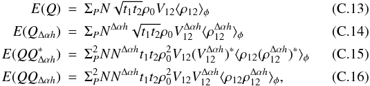 with
with
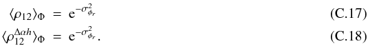 We
also have
We
also have ![Mathematical equation: \appendix \setcounter{section}{3} \begin{eqnarray} \langle \rho_{12}\rho^{\Delta\alpha{h}}_{12}\rangle _{\Phi}&=& \frac{ P_1({\vec r})P_2({\vec r}+\lambda{\vec f})P_1({\vec r}^{\prime})P_2({\vec r}^{\prime}+\lambda{{\vec f^{\prime}}})\langle \exp^{i(\phi_1({\vec r})+\phi_1({\vec r}^{\prime}+\vec{\Delta\alpha}{h})-\phi_2({\vec r}+\lambda{\vec f})-\phi_2({\vec r}^{\prime}+\lambda{{\vec f^{\prime}}}+\vec{\Delta\alpha}{h}))}\rangle _{\Phi}\mathrm{d}{\vec r}\mathrm{d}{\vec r^{\prime}}\mathrm{d}{\vec f}\mathrm{d}{\vec f}^{\prime}}{\left[\int P_1({\vec r})\mathrm{d}{\vec r} \int P_2({\vec r})\mathrm{d}{\vec r}\right]^2}\nonumber\\ &=&\mathrm{e}^{-4\sigma^2_{\phi_r}}\frac{\int P_1({\vec r})P_2({\vec r}+\lambda{\vec f})P_1({\vec r}^{\prime})P_2({\vec r}^{\prime}+\lambda{{\vec f^{\prime}}})\exp^{\frac{1}{2}\mathcal{D}_{\phi_r}({\vec r},{\vec r^{\prime}}+\vec{\Delta\alpha}{h})+\frac{1}{2}\mathcal{D}_{\phi_r}({\vec r}+\lambda{\vec f},{\vec r^{\prime}}+\lambda{{\vec f^{\prime}}}+\vec{\Delta\alpha}{h})}\mathrm{d}{\vec r}\mathrm{d}{\vec r^{\prime}}\mathrm{d}{\vec f}\mathrm{d}{\vec f}^{\prime}}{\left[\int P_1({\vec r})\mathrm{d}{\vec r} \int P_2({\vec r})\mathrm{d}{\vec r}\right]^2}\nonumber\\ && \mbox{change of variables}~{\vec r}+\lambda{\vec f} \rightarrow {\vec u}, {\vec r^{\prime}}+\lambda{{\vec f^{\prime}}} \rightarrow {\vec u^{\prime}}:\nonumber\\ \label{eq_rhoij2cov_mono}&=&\mathrm{e}^{-4\sigma^2_{\phi_r}}\frac{\int P_1({\vec r})P_1({\vec r}^{\prime})\exp^{\frac{1}{2}\mathcal{D}_{\phi_r}({\vec r},{\vec r^{\prime}}+\vec{\Delta\alpha}{h})}\mathrm{d}{\vec r}\mathrm{d}{\vec r^{\prime}}\int P_2({\vec r})P_2({\vec r}^{\prime})\exp^{\frac{1}{2}\mathcal{D}_{\phi_r}({\vec r},{\vec r^{\prime}}+\vec{\Delta\alpha}{h})}\mathrm{d}{\vec r}\mathrm{d}{\vec r^{\prime}}}{\left[\int P_1({\vec r})\mathrm{d}{\vec r} \int P_2({\vec r})\mathrm{d}{\vec r}\right]^2} \end{eqnarray}](/articles/aa/full_html/2010/16/aa13356-09/aa13356-09-eq359.png) (C.19)
(C.19)![Mathematical equation: \appendix \setcounter{section}{3} \begin{eqnarray} \langle \rho_{12}(\rho^{\vec{\Delta\alpha}{h}}_{12})^{\ast}\rangle _{\Phi}&=&\frac{P_1({\vec r})P_2({\vec r}+\lambda{\vec f})P_1({\vec r}^{\prime})P_2({\vec r}^{\prime}+\lambda{{\vec f^{\prime}}})\langle \exp^{i(\phi_1({\vec r})-\phi_1({\vec r}^{\prime}+\vec{\Delta\alpha}{h})-\phi_2({\vec r}+\lambda{\vec f})+\phi_2({\vec r}^{\prime}+\lambda{{\vec f^{\prime}}}+\vec{\Delta\alpha}{h}))}\rangle _{\Phi}\mathrm{d}{\vec r}\mathrm{d}{\vec r^{\prime}}\mathrm{d}{\vec f}\mathrm{d}{\vec f}^{\prime}}{\left[\int P_1({\vec r})\mathrm{d}{\vec r} \int P_2({\vec r})\mathrm{d}{\vec r}\right]^2}\nonumber\\ &=&\frac{\int P_1({\vec r})P_2({\vec r}+\lambda{\vec f})P_1({\vec r}^{\prime})P_2({\vec r}^{\prime}+\lambda{{\vec f^{\prime}}})\exp^{-\frac{1}{2}\mathcal{D}_{\phi_r}({\vec r},{\vec r^{\prime}}+\vec{\Delta\alpha}{h})-\frac{1}{2}\mathcal{D}_{\phi_r}({\vec r}+\lambda{\vec f},{\vec r^{\prime}}+\lambda{{\vec f^{\prime}}}+\vec{\Delta\alpha}{h})}\mathrm{d}{\vec r}\mathrm{d}{\vec r^{\prime}}\mathrm{d}{\vec f}\mathrm{d}{\vec f}^{\prime}}{\left[\int P_1({\vec r})\mathrm{d}{\vec r} \int P_2({\vec r})\mathrm{d}{\vec r}\right]^2}\nonumber\\ && \mbox{change of variables}~{\vec r}+\lambda{\vec f} \rightarrow {\vec u}, {\vec r^{\prime}}+\lambda{{\vec f^{\prime}}} \rightarrow {\vec u^{\prime}}:\nonumber\\ \label{eq_absrhoij2cov_mono}&=&\frac{\int P_1({\vec r})P_1({\vec r}^{\prime})\exp^{-\frac{1}{2}\mathcal{D}_{\phi_r}({\vec r},{\vec r^{\prime}}+\vec{\Delta\alpha}{h})}\mathrm{d}{\vec r}\mathrm{d}{\vec r^{\prime}}\int P_2({\vec r})P_2({\vec r}^{\prime})\exp^{-\frac{1}{2}\mathcal{D}_{\phi_r}({\vec r},{\vec r^{\prime}}+\vec{\Delta\alpha}{h})}\mathrm{d}{\vec r}\mathrm{d}{\vec r^{\prime}}}{\left[\int P_1({\vec r})\mathrm{d}{\vec r} \int P_2({\vec r})\mathrm{d}{\vec r}\right]^2}. \end{eqnarray}](/articles/aa/full_html/2010/16/aa13356-09/aa13356-09-eq360.png) (C.20)Putting
Eqs. (C.17, C.18, C.19, C.20) into
Eqs. (C.15, C.16, C.13, C.14), we find
that the covariance part of the singlemode astrometric phase writes
(C.20)Putting
Eqs. (C.17, C.18, C.19, C.20) into
Eqs. (C.15, C.16, C.13, C.14), we find
that the covariance part of the singlemode astrometric phase writes
![Mathematical equation: \appendix \setcounter{section}{3} \begin{equation} \mathrm{cov}(\phi_s, \phi_r^{\Delta\alpha{h}}) = \frac{1}{2}\frac{\left[\int P({\vec r})P({\vec r}^{\prime})\mathrm{e}^{-\frac{1}{2}\mathcal{D}_{\phi_r}({\vec r},{\vec r^{\prime}}+\vec{\Delta\alpha}{h})}\mathrm{d}{\vec r}\mathrm{d}{{\vec r^{\prime}}}\right]^2-\mathrm{e}^{-4\sigma^2_{\phi_r}}\left[\int P({\vec r})P({\vec r}^{\prime})\mathrm{e}^{\frac{1}{2}\mathcal{D}_{\phi_r}({\vec r},{\vec r^{\prime}}+\vec{\Delta\alpha}{h})}\mathrm{d}{\vec r}\mathrm{d}{{\vec r^{\prime}}}\right]^2}{\left[\int P({\vec r})\mathrm{d}{\vec r}\right]^4\mathrm{e}^{-2\sigma^2_{\phi_r}}}. \end{equation}](/articles/aa/full_html/2010/16/aa13356-09/aa13356-09-eq361.png) (C.21)
(C.21)
Appendix D: Phase spatial fluctuations in partial AO correction
The spatial fluctuations of the atmospheric phase can be characterized by the computation
of the so-called spatial structure function  , defined as the variance of the phase
difference taken at two radii r and
, defined as the variance of the phase
difference taken at two radii r and
 :
:
 (D.1)In the fully turbulent
case, and assuming Kolmogorov’s description of the atmosphere, the phase structure
function can be written (Roddier 1979)
(D.1)In the fully turbulent
case, and assuming Kolmogorov’s description of the atmosphere, the phase structure
function can be written (Roddier 1979)
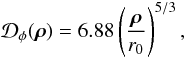 (D.2)r0
being the fried parameter, which gives the ultimate spatial resolution achievable with
atmospheric turbulence, that is
θturb = λ/r0.
When partial AO correction is applied, low (spatial) orders of the corrugated wavefront
are real-time compensated thanks to a deformable mirror. The variance
(D.2)r0
being the fried parameter, which gives the ultimate spatial resolution achievable with
atmospheric turbulence, that is
θturb = λ/r0.
When partial AO correction is applied, low (spatial) orders of the corrugated wavefront
are real-time compensated thanks to a deformable mirror. The variance
 of the residual turbulent phase
φr(r) not
corrected by the system, can be approximated as following, providing a full correction of
the first J ≪ 1 Zernike modes of the turbulence Noll (1976):
of the residual turbulent phase
φr(r) not
corrected by the system, can be approximated as following, providing a full correction of
the first J ≪ 1 Zernike modes of the turbulence Noll (1976): 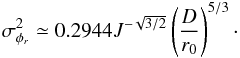 (D.3)Furthermore, the
phase structure function of the residual phase can be written as
(D.3)Furthermore, the
phase structure function of the residual phase can be written as
![Mathematical equation: \appendix \setcounter{section}{4} \begin{equation} \label{eq_aocorrel}\mathcal{D}_{\phi_r}({\vec \rho}) = 2\sigma^2_{\phi_r}\left[1-\frac{\langle \phi^r({\vec r})-\phi^r({\vec r}+{\vec \rho})\rangle }{\sigma^2_{\phi_r}}\right]\cdot \end{equation}](/articles/aa/full_html/2010/16/aa13356-09/aa13356-09-eq373.png) (D.4)For ρ
bigger than typically the distance between the mirror’s actuators, the phases are
uncorrelated, that is
⟨ φr(r) − φr(r + ρ) ⟩ = 0,
and consequently
(D.4)For ρ
bigger than typically the distance between the mirror’s actuators, the phases are
uncorrelated, that is
⟨ φr(r) − φr(r + ρ) ⟩ = 0,
and consequently  saturates at
 . The
long exposure AO corrected transfer function of the atmosphere is by definition
. The
long exposure AO corrected transfer function of the atmosphere is by definition
![Mathematical equation: \appendix \setcounter{section}{4} \begin{equation} B({\vec f}) = \exp\left[-\frac{1}{2}\mathcal{D}_{\phi_r}(\lambda{\vec f})\right]. \end{equation}](/articles/aa/full_html/2010/16/aa13356-09/aa13356-09-eq378.png) (D.5)Taking into account
the properties of the phase structure function of the residual phase,
B(f) can be decomposed in two parts
(Conan 1994): one low-frequency term – namely the
halo (FTOhalo) – and one high-frequency term
saturating at
(D.5)Taking into account
the properties of the phase structure function of the residual phase,
B(f) can be decomposed in two parts
(Conan 1994): one low-frequency term – namely the
halo (FTOhalo) – and one high-frequency term
saturating at  ,
namely the coherent energy. From this follows that the long exposure transfer function of
the telescope
T(f) = T0(f).B(f),
where T0(f) is the transfer
function of a perfect telescope, can be in first approximation modelled by a sum of two
components:
,
namely the coherent energy. From this follows that the long exposure transfer function of
the telescope
T(f) = T0(f).B(f),
where T0(f) is the transfer
function of a perfect telescope, can be in first approximation modelled by a sum of two
components: ![Mathematical equation: \appendix \setcounter{section}{4} \begin{eqnarray} T(f) &=& T_0(f).[{\rm e}^{-\sigma^2_{\phi_r}} + FTO_{\rm halo}(f)] \nonumber \\ &\simeq& T_0(f).[{\rm e}^{-\sigma^2_{\phi_r}}+ (1-\exp^{-\sigma^2_{\phi_r}})\exp^{-\frac{1}{2}\mathcal{D}_{\phi}(\lambda{\vec f})}]. \end{eqnarray}](/articles/aa/full_html/2010/16/aa13356-09/aa13356-09-eq384.png) (D.6)Equation (D.4) also demonstrates that for
interferometers equipped with AO systems, the phases
(D.6)Equation (D.4) also demonstrates that for
interferometers equipped with AO systems, the phases  and
and
 of telescopes 1 and 2 are
always uncorrelated. As a consequence, the phase structure function of the residual piston
phase
of telescopes 1 and 2 are
always uncorrelated. As a consequence, the phase structure function of the residual piston
phase  is twice
the phase structure function of the residual phase over one single telescope (assuming
equivalent AO systems for both telescopes), that is
is twice
the phase structure function of the residual phase over one single telescope (assuming
equivalent AO systems for both telescopes), that is  . Indeed, even if no AO correction is applied,
the phases φ1 and φ2 can still be
considered to be uncorrelated, as soon as the baseline is longer than the outer scale of
the atmosphere ℒ0. This is for example the case for the VLTI at Paranal, where
the outer scale has been estimated to be ℒ0 ≃ 22 m (Martin et al. 2000).
. Indeed, even if no AO correction is applied,
the phases φ1 and φ2 can still be
considered to be uncorrelated, as soon as the baseline is longer than the outer scale of
the atmosphere ℒ0. This is for example the case for the VLTI at Paranal, where
the outer scale has been estimated to be ℒ0 ≃ 22 m (Martin et al. 2000).
All Tables
Expression of the variance of the phase for the three noise regimes, the detector, photon, and atmospheric regimes, both in the multimode and singlemode cases.
Parameters a and σ of the Rician probability distribution function for both multimode and singlemode cases.
All Figures
|
Fig. 1 Sketch of the effect of the turbulence in interferometry. On each telescope pupil
P(r) separated by the baseline
distance B12, the wavefront is affected by a random phase
screen, respectively φ1(r)
and φ2(r). The strength of
the turbulence depends on the parameters
D/r0 where
D is the diameter of the telescope
and r0 is the Fried parameter (Fried 1965), describing the typical size of a coherent cell in the
wavefront. Furthermore, the optical path difference between the two beams is randomly
shifted by the turbulent piston |
| In the text | |
|
Fig. 2 Global performance comparison between multimode and singlemode
interferometry, all sources of noise considered. Top: error of the
phase in multimode (dotted lines) and singlemode (solid lines) as the function of
the number of detected photoevents (per time unit) and K-band
magnitude. For both cases, we can see the three regimes: the detector noise (in
1/N), then (shortly) the photon noise (in
|
| In the text | |
|
Fig. 3 Limiting flux as a function of the Strehl ratio (detector noise regime case) for turbulence strengths of D/r0 = 8 (left) and D/r0 = 2 (right). Plots are shown for an unresolved (V = 1), fairly resolved (V = 0.5), and fully resolved (V = 0.1) source, respectively. Curves are going by pair for singlemode (solid lines) and multimode (dotted lines) cases. The fixed parameters have the same values as previous figures. |
| In the text | |
|
Fig. 4 Phase speckle noise as a function of the Strehl ratio for both singlemode (solid line) and multimode (dotted line) cases, with D/r0 = 8. The ratio between the multimode and the singlemode phase errors is plotted in dashed line (y-axis on the right side). |
| In the text | |
|
Fig. 5 Long exposure visibility attenuation owing to the atmospheric noise of the measurement of the phase, as a function of the Strehl ratio for multimode (dotted line) and singlemode (solid line) systems, with D/r0 = 8. The ratio of the attenuation between singlemode and multimode is plotted in a dashed line (y-axis on the right side). |
| In the text | |
|
Fig. 6 Density probability of the multimode instantaneous Strehl ratio (I = |T12| 2, red lines) and singlemode one (I = |ρ12| 2, black lines) for various levels of AO correction and turbulence strengths. Top: constant turbulence strength D/r0 = 8 and the number of corrected Zernike are, from left to right, nz = 10,15,30. Bottom: constant AO correction nz = 3 (tip-tilt only), with various turbulence strengths, from left to right D/r0 = 8,4,2. |
| In the text | |
|
Fig. 7 Left: probability for the instantaneous interferometric Strehl ratio I to be lower than the value ϵ for the tip-tilt correction only, for different strengths of turbulence D/r0 = 8,4,2 (respectively in blue, magenta and red), for the multimode (dotted line) and singlemode (solid line) cases. Right: multimode versus singlemode probability ratio. |
| In the text | |
|
Fig. 8 Left: astrometric phase error caused by atmospheric turbulence, as the function of the angular distance Δα between the source and the reference star for both singlemode (solid lines) and multimode (dotted lines). Right: ratio of the multimode versus the singlemode astrometric error. Results are shown for various AO correction levels as described in the figures above. We have assumed one single turbulent layer located at h = 10 km. |
| In the text | |
Current usage metrics show cumulative count of Article Views (full-text article views including HTML views, PDF and ePub downloads, according to the available data) and Abstracts Views on Vision4Press platform.
Data correspond to usage on the plateform after 2015. The current usage metrics is available 48-96 hours after online publication and is updated daily on week days.
Initial download of the metrics may take a while.