| Issue |
A&A
Volume 523, November-December 2010
|
|
|---|---|---|
| Article Number | A35 | |
| Number of page(s) | 4 | |
| Section | Planets and planetary systems | |
| DOI | https://doi.org/10.1051/0004-6361/201015148 | |
| Published online | 15 November 2010 | |
Selective principal component extraction and reconstruction: a novel method for ground based exoplanet spectroscopy
1
Woodruff School of Mechanical Engineering, MRDC Building, Room 4111,
Georgia Institute of Technology,
Atlanta,
Georgia
30332-0405,
USA
e-mail: This email address is being protected from spambots. You need JavaScript enabled to view it.
2
Jet Propulsion Laboratory, California Institute of Technology,
4800 Oak Grove
Drive, Pasadena,
California
91109-8099,
USA
Received:
3
June
2010
Accepted:
12
August
2010
Abstract
Context. Infrared spectroscopy of primary and secondary eclipse events probes the composition of exoplanet atmospheres and, using space telescopes, has detected H2O, CH4 and CO2 in three hot Jupiters. However, the available data from space telescopes has limited spectral resolution and does not cover the 2.4 − 5.2μm spectral region. While large ground based telescopes have the potential to obtain molecular-abundance-grade spectra for many exoplanets, realizing this potential requires retrieving the astrophysical signal in the presence of large Earth-atmospheric and instrument systematic errors.
Aims. Here we report a wavelet-assisted, selective principal component extraction method for ground based retrieval of the dayside spectrum of HD 189733b from data containing systematic errors.
Methods. The method uses singular value decomposition and extracts those critical points of the Rayleigh quotient which correspond to the planet induced signal. The method does not require prior knowledge of the planet spectrum or the physical mechanisms causing systematic errors.
Results. The spectrum obtained with our method is in excellent agreement with space based measurements made with HST and Spitzer and confirms the recent ground based measurements including the strong ~ 3.3μm emission.
Key words: infrared: planetary systems / planets and satellites: atmospheres / techniques: spectroscopic / methods: data analysis / methods: numerical
© ESO, 2010
1. Introduction
Detection of molecules in exoplanet atmospheres via infrared spectroscopy from space-based telescopes is now routine (Swain et al. 2008; Grillmair et al. 2008; Swain et al. 2009b,a; Tinetti et al. 2010). Recently, Swain et al. (2010) demonstrated molecular spectroscopy of an exoplanet atmosphere with ground-based measurements. With the availability of numerous large ground based telescopes equipped with infrared spectrometers, there is a great potential to obtain a large quantity of “molecular-abundance-grade” spectra; realizing this potential requires developing optimal signal extraction algorithms to retrieve the spectral signature of an exoplanet atmosphere in the presence of large Earth-atmospheric and instrument systematic errors. Here we present a method based on principal component analysis (PCA) capable of detecting the exoplanet emission spectrum from the ground. PCA is a well established method with numerous astronomomical applications; it has been used to search for an exoplanet signal in ground-based spectroscopic observations (Brown et al. 2002) and a related method is used in SysRem for exoplanet eclipse detections (Tamuz et al. 2005). We apply our PCA based method to extract the dayside emission spectrum of HD 189733b in the K and L bands and we compare the resulting spectrum with previously reported results (Swain et al. 2010), which were obtained using a different method.
2. Observations and initial calibration
The spectrum presented here is based on the same observations used in Swain et al. (2010) but analyzed using the selective principal component extraction and reconstruction (SPCER) method described in Sect. 3. A secondary eclipse of HD 189733b was observed on August 11th, 2007 using the SpeX instrument mounted on the NASA Infrared Telescope Facility (IRTF). The spectroscopic time series begins approximately one hour before the onset of ingress and ends approximately one hour after the termination of egress. The details of the observations and the reduction with SpexTool are presented in Swain et al. (2010). The result of the standard SpexTool calibration is a flux density time series with ~ 4% variations. We then employ the initial calibration step (normalization & airmass correction) outlined in Swain et al. (2010). Finally, we separate the exoplanet eclipse astrophysical signal from the residual systematic errors using the SPCER method and thus obtain the exoplanet emission spectrum.
3. Method
The astrophysical signal from the exoplanet is present in all spectral channels and we have developed the SPCER method to identify this signal (i.e. the exoplanet eclipse) and separate it from other signal components which are not of astrophysical origin and present in all spectral channels (i.e. systematic errors). The method is based on principal component analysis (PCA), which performs an orthogonal transformation that aligns the transformed axes in the directions of maximum variance. From statistical viewpoint, the eigenvectors of the covariance matrix of a dataset are the critical points of the Rayleigh quotient and when ranked according to the magnitude of the eigenvalues, they represent the axes of maximum variance of that data. To successfully separate non-random signals (systematic errors; the astrophysical signal) from random noise, it is desirable that the time series data has a high signal to noise (SNR) ratio. Therefore, we prefilter the time series prior to applying the SPCER method. After prefiltering, we perform singular value decomposition of a set of time series at different wavelengths. This conventiently separates the astrophysical signal from some of the larger systematic errors present in the data. We then reconstruct the astrophysical signal dominated time series and measure the exoplanet emission spectrum. In this section, we outline the methodology. In Sect. 4, we discuss the results of applying this method to the HD 189733b dataset.
3.1. Prefiltering
To clean the time series and at the same time retain the dynamic features of the data, we
have implemented wavelet transform based adaptive signal extraction. Wavelets are
time-localized because the supports of wavelet functions are finite. This makes wavelets
excellent for representing discrete events (e.g. abrupt changes linked to outlier points).
The wavelet basis functions are constructed from a single function, termed the “Mother
Wavelet”, ψ0,0. The time series is represented as a set of
wavelet functions, ψj,k, constructed by a
combination of dilation and translation of the mother function:
ψj,k = 2j / 2ψ0,0(2jt − k).
Here, we implemented the standard wavelet decomposition-thresholding-reconstruction
procedure which is widely used in signal and image processing fields (Sidney et al. 1998; Mallat 1989, 1999; Donoho 1995; Donoho & Johnstone
1995). As mother wavelet, we use the standard Daubechies 3 wavelet (Mallat 1999). We obtain the wavelet decomposition by a
multi-scale representation and using the transform coefficients  (kth scaling
function at jth scale) and
(kth scaling
function at jth scale) and  (kth wavelet
function at jth scale) defined as,
(kth wavelet
function at jth scale) defined as, 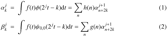 where
the scaling function φ can be respresented as a signal with a low-pass
spectrum and expressed in terms of wavelets (see Mallat
1989); f(t) is the time series for a specific
wavelength. h(n) and
g(n) represent low pass and high pass filter
coefficients respectively and are obtained using Daubechies 3 wavelets in MATLAB. For a
detailed description on the theory of wavelet decomposition, the reader is referred to
Sidney et al. (1998); Mallat (1989). To produce a smoother estimate and continuous mapping
during wavelet shrinkage, we implement a soft thresholding scheme,
ηT(wj) = sign(wj)( | wj | − T) + ,
where wj is substituted by the different
and , along with the universal
threshold
where
the scaling function φ can be respresented as a signal with a low-pass
spectrum and expressed in terms of wavelets (see Mallat
1989); f(t) is the time series for a specific
wavelength. h(n) and
g(n) represent low pass and high pass filter
coefficients respectively and are obtained using Daubechies 3 wavelets in MATLAB. For a
detailed description on the theory of wavelet decomposition, the reader is referred to
Sidney et al. (1998); Mallat (1989). To produce a smoother estimate and continuous mapping
during wavelet shrinkage, we implement a soft thresholding scheme,
ηT(wj) = sign(wj)( | wj | − T) + ,
where wj is substituted by the different
and , along with the universal
threshold  ,
where N is the current level of wavelet decomposition and
σN is the approximation of noise at this
level obtained using the robust median estimator. After thresholding, we reconstruct the
time series using reconstruction filters and the iterative reconstruction method. Our
wavelet based signal extraction algorithm accepts signal
Fλ(t) as input and
returns the de-noised signal
,
where N is the current level of wavelet decomposition and
σN is the approximation of noise at this
level obtained using the robust median estimator. After thresholding, we reconstruct the
time series using reconstruction filters and the iterative reconstruction method. Our
wavelet based signal extraction algorithm accepts signal
Fλ(t) as input and
returns the de-noised signal  . As a result of this procedure, we get on
average a 56% improvement in the
. As a result of this procedure, we get on
average a 56% improvement in the  of the
individual time series measurements.
of the
individual time series measurements.
3.2. Separating multiple patterns in the data
We start by averaging the time series in the spectral domain (mean of 5 adjacent
spectral channels) to reduce the number of PCs and get the time series
 . Given X, a subset of
composed of P spectral
channels, we center X by subtracting
. Given X, a subset of
composed of P spectral
channels, we center X by subtracting  ,
the mean of each column of X. Through singular value decomposition we
find the eigenvalues (
,
the mean of each column of X. Through singular value decomposition we
find the eigenvalues ( ) and the eigenvectors (principal components
 ) of the covariance matrix of X.
We then project the centered data onto the principal component axes to get
) of the covariance matrix of X.
We then project the centered data onto the principal component axes to get
 ,
the representation of X in the principal component space using
,
the representation of X in the principal component space using  where ⊗ denotes matrix multiplication.
For our purposes, we want to decompose the signal present in the ensemble of time series
into various components, e.g. flux variation due to secondary eclipse and
Earth-atmospheric effects etc. For this, we transform each individual principal component
 into the time domain as,
 (3)At this point, what we
have done is transform our set of time series so that it is expressed in terms of patterns
(principal components) that optimally represent the covariance (commonality) of
X. Each
(3)At this point, what we
have done is transform our set of time series so that it is expressed in terms of patterns
(principal components) that optimally represent the covariance (commonality) of
X. Each  is such a
reconstructed pattern and it shows how the signal would have looked like if it was due to
this single PC. We can now determine which PCs represent the eclipse and which represent
confusing systematic errors.
is such a
reconstructed pattern and it shows how the signal would have looked like if it was due to
this single PC. We can now determine which PCs represent the eclipse and which represent
confusing systematic errors.
3.3. Extracting the exoplanet spectrum
To select the principal components corresponding to the eclipse, we calculate the linear
correlation coefficient (CC) between each of the individually
reconstructed signals and the
expected light curve shape. No prior knowledge on the depth of the eclipse is required for
this; only the exoplanet ephemerides(Winn et al.
2007, for HD 189733) is needed. We select a set of principal components capturing
the eclipse event using selection criteria described below and reconstruct the data using
these components ( ). As a result of this
reconstruction, we get an exoplanet eclipse light curve in which the effect of confusing
systematics is greatly reduced. For each wavelength channel in
X, we determine the eclipse depth and the error bar based on the
standard deviation of the time series in-eclipse and out-of-eclipse. The eclipse depth for
X is the average eclipse depth and the error bar is composed of the
error on the eclipse depth for each wavelength channel and the standard deviation of the
depths for each wavelength channel in X:
). As a result of this
reconstruction, we get an exoplanet eclipse light curve in which the effect of confusing
systematics is greatly reduced. For each wavelength channel in
X, we determine the eclipse depth and the error bar based on the
standard deviation of the time series in-eclipse and out-of-eclipse. The eclipse depth for
X is the average eclipse depth and the error bar is composed of the
error on the eclipse depth for each wavelength channel and the standard deviation of the
depths for each wavelength channel in X:
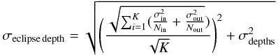 (4)with
σin and σout the standard
deviation of the flux in-eclipse and out-eclipse regions for each wavelength channel in
X; Nin and Nout
the number of observations in and out of eclipse; K the number of
wavelength channels in X; σdepths the
standard deviation of the eclipse depth for the different wavelength channels
in X.
(4)with
σin and σout the standard
deviation of the flux in-eclipse and out-eclipse regions for each wavelength channel in
X; Nin and Nout
the number of observations in and out of eclipse; K the number of
wavelength channels in X; σdepths the
standard deviation of the eclipse depth for the different wavelength channels
in X.
The selection criteria to decide whether a principal component captures the exoplanet eclipse event are:
-
1.
| CC | PC,i > | CC | threshold, with | CC | threshold = mean( | CC | ) + stddev( | CC | ); the correlation coefficient of the PC must be large enough, such that it describes well the eclipse event;
-
2.
RPC,i < Rthreshold with RPC,i the eigenvalue rank of the ith selected PC and Rthreshold is the cutoff value for rank. We have chosen Rthreshold = 9 (see later);
-
3.
| RPC,i − RPC,i + 1 | < Δthreshold; Δthreshold is the cutoff value for the difference in the ranks of the selected PCs. We have chosen Δthreshold = 6 (see later).
If no PC is found under these selection criteria, we assign an upper limit to the eclipse depth, matching the lowest eclipse depth found in the dataset and conclude that we could not find the eclipse for those wavelength channels.
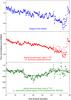 |
Fig. 1 Separating the astrophysical signal from systematic errors. The different panels depict: top: an original, normalized and airmass corrected time series, middle: signal reconstructed using the first PC, bottom: signal reconstructed using the second PC. In the bottom panel, we show using a black dashed line the secondary eclipse lightcurve overplotted on the reconstructed data. The singular value decomposition of a set of time series at different wavelengths allows us to extract the exoplanet signature, largely free of systematic errors. We show the data at the original, unbinned time sampling. |
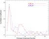 |
Fig. 2 Selecting the principal components which capture the exoplanet eclipse. The linear correlation coefficients between the PCs and the model eclipse light curve are shown for representative wavelengths for the K and L-band. The eclipse is captured by PCs with a high correlation coefficient. The selection of PCs is rather straightforward with very large correlation coefficients being found at low PC numbers. |
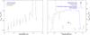 |
Fig. 3 Dayside emission spectrum. The K-band (left) and L-band (right) HD 189733b emission spectrum obtained using SPCER is shown using green squares and is compared to the space-based HST spectrum (Swain et al. 2009a) and Spitzer broad-band photometry (Charbonneau et al. 2008) and the ground-based spectrum reported in Swain et al. (2010). We also show the Spitzer passband (blue line) for the 3.6μm photometric point and have averaged the SPCER result over this passband to make comparison easy (blue open symbol). There is excellent agreement between the space and ground-based datasets. |
4. Results and discussion
We have applied the method outlined above to the spectroscopic time series on the secondary eclipse of HD 189733b observed with the IRTF. We chose to use the same spectral binning as in Swain et al. (2010), such that we can easily compare the results. In the K-band and L-band, we used 100 and 150 spectral channels respectively to construct X. We then processed the data through the different steps outlined above and a sample result of the principal component extraction is shown in Fig. 1. Blue symbols show the normalized original light curve which is dominated by residual systematic errors. Red and green curves show the signal reconstructed using the first and the second PC respectively. The model eclipse curve is shown in black. The first PC can be seen to represent much of the systematic errors present in the original signal, while the second PC is clearly the exoplanet eclipse. This demonstrates the potential of SPCER in separating systematic effects for ground based observations and in retrieving the exoplanet signal. It does so without requiring knowledge of the physical mechanism causing the corruption nor requiring prior knowledge on the exoplanet.
To determine the exoplanet spectrum, we have selected using the
criterium outlined above with Rthreshold = 9 and
Δthreshold = 6. In Fig. 2, we illustrate
the calculated correlation coefficients with the light curve for K and
L-band wavelengths. It is clearly seen that a PC either matches really
well (CC > 0.65) or not very well, making the selection rather
straightforward and changes in the selection criterium have little influence. The result of
the procedure, the exoplanet spectrum of HD 189733b, is shown in Fig. 3. The SPCER method reproduces the measurements by HST (Swain et al. 2009a), the Spitzer photometry (Charbonneau et al. 2008) and those reported in (Swain et al. 2010) extremely well, within the error bars.
A few considerations we would like to mention are:
-
Importance of pre-cleaning the data; removing the biggesterrors first. The data processing outlined in Swainet al. (2010) includes removal ofsystematic errors correlated in wavelength and airmass. If thisstep is not taken, it is still feasible to find the eclipse signal, but atlower eigenvalue rank. For instance, not performing the airmasscorrection outlined in Swainet al. (2010), shifts the eclipsesignal from a typical eigenvalue rank 2 to eigenvalue rank 4.
-
Importance of selecting (sometimes) multiple PCs. There is a lack of control in the choice of orthogonal basis functions in the singular value decomposition. This means that the eclipse is not always captured in a single PC, and several PCs (typically two) may be needed to represent the eclipse. When the reconstruction is done based solely on one PC, the spectral shape is preserved, but the average eclipse depth can change by up to ~ 20%.
-
Possible improvement by post-processing the PCs. The SPCER method does not necessarily decompose the data entirely into an eclipse and non-eclipse component, because no priors are included (which is also the strength of the method). As such, some residual systematic error can be convolved with the eclipse signal. Simple post-processing, like fitting a polynomial to the out-of-eclipse part of the light curve, can potentially enhance the SNR of the exoplanet spectrum. For this particular dataset, this was not necessary, but might prove advantageous for other datasets.
-
Further improvements are likely possible by incorporating the known eclipse shape. In the method presented here, no prior knowledge of the eclipse shape is used during the disentanglement of systematic effects and eclipse signal. Methods that incorporate priors, such as an iterative matched filter, have the potential to improve the method presented here.
-
Equal signal to noise ratio for the different wavelength channels is assumed when using PCA. For the dataset analyzed here, the different wavelength channels in each spectral bin X differ only marginally in count rate (the standard deviation of the normalized SNR is on average 4% and is always less than 13% for the different wavelength bins X) and regular PCA is therefore appropriate. If this is not the case, a SysRem type of down-weighting of wavelength channels with low count rates (Tamuz et al. 2005), is needed.
In summary, the coupled wavelet denoising-SPCER method presented here is a new and powerful method for ground based exoplanet calibration. A useful aspect of the method lies in its ability to reject systematic errors without the need for knowledge of the underlying physical mechanism. This gives us the ability
to separate the original planetary signal from the relatively large systematic effects. The results of the SPCER-based calibration for the emission spectrum of HD 189733b are in excellent agreement with those obtained with HST (Swain et al. 2009b) and Spitzer (Charbonneau et al. 2008) and confirm the recent ground based measurements (Swain et al. 2010). The strength of SPCER in retrieving the exoplanet spectrum from ground based observations is a proof of concept for its more general application in fields where signal deeply buried under noise must be extracted; the method has applications in a variety of fields including earth and atmospheric sciences, telecommunication systems, measurement instruments, biomedical engineering, optics, image processing and controls, where problems of not having good signal to noise ratio before signal amplification are prevalent or where pattern recognition is critical.
References
- Brown, T. M., Libbrecht, K. G., & Charbonneau, D. 2002, PASP, 114, 826 [NASA ADS] [CrossRef] [Google Scholar]
- Charbonneau, D., Knutson, H. A., Barman, T., et al. 2008, ApJ, 686, 1341 [NASA ADS] [CrossRef] [MathSciNet] [Google Scholar]
- Donoho, D. L. 1995, IEEE Transactions on information theory, 41, 613 [Google Scholar]
- Donoho, D. L., & Johnstone, I. M. 1995, J. Amer. Statist. Assoc., 90, 1200 [Google Scholar]
- Grillmair, C. J., Burrows, A., Charbonneau, D., et al. 2008, Nature, 456, 767 [NASA ADS] [CrossRef] [PubMed] [Google Scholar]
- Mallat, S. G. 1989, IEEE Transactions on Pattern Analysis and Machine Intelligence, 11, 674 [Google Scholar]
- Mallat, S. G. 1999, A Wavelet Tour of Signal Processing, 2nd edn. (Associated Press) [Google Scholar]
- Sidney, B., Ramesh, A. G., & Haitao, G. 1998, Introduction to Wavelets and Wavelet Transforms: A Primer (Prentice-hall International) [Google Scholar]
- Swain, M. R., Vasisht, G., & Tinetti, G. 2008, Nature, 452, 329 [NASA ADS] [CrossRef] [PubMed] [Google Scholar]
- Swain, M. R., Tinetti, G., Vasisht, G., et al. 2009a, ApJ, 704, 1616 [NASA ADS] [CrossRef] [Google Scholar]
- Swain, M. R., Vasisht, G., Tinetti, G., et al. 2009b, ApJ, 690, L114 [NASA ADS] [CrossRef] [Google Scholar]
- Swain, M. R., Deroo, P., Griffith, C. A., et al. 2010, Nature, 463, 637 [NASA ADS] [CrossRef] [PubMed] [Google Scholar]
- Tamuz, O., Mazeh, T., & Zucker, S. 2005, MNRAS, 356, 1466 [NASA ADS] [CrossRef] [Google Scholar]
- Tinetti, G., Deroo, P., Swain, M. R., et al. 2010, ApJ, 712, L139 [NASA ADS] [CrossRef] [Google Scholar]
- Winn, J. N., Holman, M. J., Henry, G. W., et al. 2007, AJ, 133, 1828 [NASA ADS] [CrossRef] [Google Scholar]
All Figures
|
Fig. 1 Separating the astrophysical signal from systematic errors. The different panels depict: top: an original, normalized and airmass corrected time series, middle: signal reconstructed using the first PC, bottom: signal reconstructed using the second PC. In the bottom panel, we show using a black dashed line the secondary eclipse lightcurve overplotted on the reconstructed data. The singular value decomposition of a set of time series at different wavelengths allows us to extract the exoplanet signature, largely free of systematic errors. We show the data at the original, unbinned time sampling. |
| In the text | |
|
Fig. 2 Selecting the principal components which capture the exoplanet eclipse. The linear correlation coefficients between the PCs and the model eclipse light curve are shown for representative wavelengths for the K and L-band. The eclipse is captured by PCs with a high correlation coefficient. The selection of PCs is rather straightforward with very large correlation coefficients being found at low PC numbers. |
| In the text | |
|
Fig. 3 Dayside emission spectrum. The K-band (left) and L-band (right) HD 189733b emission spectrum obtained using SPCER is shown using green squares and is compared to the space-based HST spectrum (Swain et al. 2009a) and Spitzer broad-band photometry (Charbonneau et al. 2008) and the ground-based spectrum reported in Swain et al. (2010). We also show the Spitzer passband (blue line) for the 3.6μm photometric point and have averaged the SPCER result over this passband to make comparison easy (blue open symbol). There is excellent agreement between the space and ground-based datasets. |
| In the text | |
Current usage metrics show cumulative count of Article Views (full-text article views including HTML views, PDF and ePub downloads, according to the available data) and Abstracts Views on Vision4Press platform.
Data correspond to usage on the plateform after 2015. The current usage metrics is available 48-96 hours after online publication and is updated daily on week days.
Initial download of the metrics may take a while.