| Issue |
A&A
Volume 523, November-December 2010
|
|
|---|---|---|
| Article Number | A77 | |
| Number of page(s) | 12 | |
| Section | Atomic, molecular, and nuclear data | |
| DOI | https://doi.org/10.1051/0004-6361/201015123 | |
| Published online | 18 November 2010 | |
Radiolysis of H2O:CO2 ices by heavy energetic cosmic ray analogs
1
IP&D/UNIVAP, Av. Shishima Hifumi, 2911, São
Jose dos Campos,
SP,
Brazil
e-mail: This email address is being protected from spambots. You need JavaScript enabled to view it.
2
Grupo de Física e Astronomia, CEFET/Química de
Nilópolis, Rua Lúcio Tavares, 1052,
CEP 2653-060, Nilópolis, Brazil
3
Centre de Recherche sur les Ions, les Matériaux et la Photonique
(CEA/CNRS/ENSICAEN/Université de Caen-Basse Normandie), CIMAP – CIRIL – GANIL, Boulevard Henri
Becquerel, BP
5133, 14070
Caen Cedex 05,
France
4
Departamento de Física, Pontifícia Universidade Católica do Rio de
Janeiro (PUC-Rio), Rua Marquês de
São Vicente 225, CEP
22453-900, Rio de Janeiro,
Brazil
Received:
1
June
2010
Accepted:
3
August
2010
Abstract
An experimental study of the interaction of heavy, highly charged, and energetic ions (52 MeV 58Ni13+) with pure H2O, pure CO2 and mixed H2O:CO2 astrophysical ice analogs is presented. This analysis aims to simulate the chemical and the physicochemical interactions induced by heavy cosmic rays inside dense and cold astrophysical environments, such as molecular clouds or protostellar clouds. The measurements were performed at the heavy ion accelerator GANIL (Grand Accélérateur National d’Ions Lourds in Caen, France). The gas samples were deposited onto a CsI substrate at 13 K. In-situ analysis was performed by a Fourier transform infrared (FTIR) spectrometer at different fluences. Radiolysis yields of the produced species were quantified. The dissociation cross sections of pure H2O and CO2 ices are 1.1 and 1.9 × 10⁻¹³ cm2, respectively. For mixed H2O:CO2 (10:1), the dissociation cross sections of both species are about 1 × 10-13 cm2. The measured sputtering yield of pure CO2 ice is 2.2 × 10⁴ molec ion-1. After a fluence of 2−3 × 10¹² ions cm-2, the CO2/CO ratio becomes roughly constant (~0.1), independent of the initial CO2/H2O ratio. A similar behavior is observed for the H2O2/H2O ratio, which stabilizes at 0.01, independent of the initial H2O column density or relative abundance.
Key words: astrochemistry / molecular data / solar wind / cosmic rays / ISM: molecules / planets and satellites: composition
© ESO, 2010
1. Introduction
H2O and CO2 are most abundant constituents of icy grain mantles in the interstellar medium (Whittet et al. 1996; Ehrenfreund & Charnley 2000). Following Gerakines et al. (1999), a significant fraction of interstellar solid CO2 exists in mixtures dominated by H2O in both quiescent cloud and protostellar regions. In those regions the relative abundance of CO2 with respect to H2O ranges from 4% to 25%.
Inside the solar system the presence of H2O and CO2 ices is also ubiquitous. For example, CO2 is widely detected in cometary ices. Its abundance, relative to H2O, is about 6−7% in the comets Hale-Bopp (Crovisier et al. 1997; Crovisier 1998) and Hyakutake (Bockelée-Morvan 1997). The H2O and CO2 ice features have been observed also in the IR spectra of the icy Galilean satellites Europa, Ganymede, Callisto (Carlson et al. 1999; McCord et al. 1998), Triton – the largest moon of Neptune (Quirico et al. 1999) – and on the surface of Mars (Herr & Pimentel 1969; Larson & Fink 1972).
Deep inside dense molecular clouds and protostellar disks, as well as on the surfaces of solar system bodies surrounded by thick atmospheres, the frozen compounds are protected from stellar energetic UV photons. However, X-rays and energetic cosmic rays can penetrate deeper and trigger molecular dissociation, chemical reactions, and evaporation processes. For solar system ices without significant atmospheres, such as Europa, Enceladus, and Oort cloud comets, the material protection to UV photons is supplied by the upper layers (tens of nm) of ice, and only the energetic particles reach the inner layers (e.g., 52 MeV Ni penetrate roughly 20 μm in pure water ice). These ices are directly exposed to stellar photons, cosmic rays, solar wind (~1 keV/amu ionized particles), and energetic solar particles and/or planetary magnetosphere particles.
Laboratory studies and astronomical observations indicate that photolysis and radiolysis of such ices can create simple molecules, such as CO, CO3, O3, H2CO3, and H2O2, and other more complex organic compounds such as formic acid, formaldehyde, methanol, etc. (e.g. Gerakines et al. 2000; Moore & Hudson 2000; Brucato et al. 1997; Wu et al. 2003). By comparing laboratory data (production rates, formation cross section, and half-lives for these compounds) with astronomical observation, we will better understand the physicochemical processes occurring in the astronomical sources.
In this work, we present infrared measurements of two different mixtures of H2O:CO2 ices, as well as of pure water and CO2 ices, irradiated by 52 MeV 58Ni13+. In Sect. 2, the experimental setup is briefly described. The infrared spectra of frozen sample measured as a function of ion fluences are the subject of Sect. 3. Section 4 has a discussion of the dissociation cross sections and other radiolysis-induced effects, as well as of the formation of new species on ices. Astrophysical implication is discussed in Sect. 5. Final remarks and conclusions are given in Sect. 6.
2. Experimental
To simulate the effects of heavy and highly ionized cosmic rays on astrophysical cold surfaces, we used the facilities at the heavy ion accelerator GANIL (Grand Accélérateur National d’Ions Lourds, Caen, France). The gas samples (purity superior to 99%) were deposited onto a CsI substrate at 13 K through a facing gas inlet. The sample-cryostat system can be rotated 180° and fixed at three different positions to allow i) gas deposition; ii) FTIR measurement; and iii) perpendicular ion irradiation.
58Ni13+ ion projectiles with energies of 52 MeV impinge perpendicularly onto both H2O:CO2 ice (1:1), H2O:CO2 ice (10:1) and onto pure H2O and CO2 ices. The target ionizing effects of Ni and Fe projectiles, at the same velocity, are almost identical since they almost have the same atomic number (Seperuelo Duarte et al. 2010). The incoming charge state 13 + corresponds approximately to the equilibrium charge state after several collisions of 52 MeV Ni atoms (independent of the initial charge state) with matter (e.g. Nastasi et al. 1996).
In-situ analysis was performed by the Nicolet FTIR spectrometer (Magna 550) from 4000 to 600 cm-1 with a resolution of 1 cm-1. The spectra were collected at different fluences up to 2 × 10¹³ ions cm-2. The Ni ion flux was 2 × 109 cm-2 s-1. During the experiment the chamber pressure was below 2 × 10⁻⁸ mbar owing to the cryopumping by the thermal shield. More details are given elsewhere (Seperuelo Duarte et al. 2009; Pilling et al. 2010).
Assuming an average density for the pure water ice and water-rich ice samples of 1 g/cm3 and 1.8 g/cm3 for the pure CO2 ice, the thickness, and the deposition rate are determined by using the initial molecular column density of the samples. For H2O:CO2 (1:1) and H2O:CO2 (10:1), the sample thicknesses were 0.6 and 0.4 μm. The deposition rates were roughly 7 and 3 μm/h, respectively. For pure H2O ice and pure CO2 ice, the thicknesses were about 0.5 and 0.4 μm, and the deposition rates were 4 and 3 μm/h, respectively. The penetration depth of 52 MeV Ni ions is much greater than ice thicknesses, therefore the ions pass though the target with approximately the same velocity (constant cross sections).
The molecular column density of a sample was determined from the relation between optical depth τν = ln(I0 / I) and the band strength, A (cm molec-1), of the respective sample vibrational mode (see d’Hendecourt & Allamandola 1986). In this expression, I and I0 are the intensity of light at a specific frequency before and after passing through a sample, respectively. Since the absorbance measured by the FTIR spectrometer is Absν = log (I0 / I), the molecular column density of ice samples is given by ![Mathematical equation: \begin{equation} N= \frac{1}{A} \int \tau_\nu {\rm d}\nu = \frac{2.3}{A} \int Abs_\nu {\rm d}\nu \quad [{\rm molec~cm^{-2}}], \label{eq-N} \end{equation}](/articles/aa/full_html/2010/15/aa15123-10/aa15123-10-eq29.png) (1)where Absν = ln(I0 / I) / ln(10) = τν / 2.3.
(1)where Absν = ln(I0 / I) / ln(10) = τν / 2.3.
The vibrational band positions and their infrared absorption coefficients (band strengths) used in this work are given in Table 1.
Infrared absorption coefficients (band strengths) used in the column density calculations for the observed molecules.
3. Results
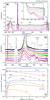 |
Fig. 1 a) Infrared spectra of H2O:CO2 13 K ice (1:1) before (top dark line) and after different irradiation fluences. b) Expanded view from 2200 to 1000 cm-1. c) Molecular column densities derived from the infrared spectra during the experiment. The lines are added to guide the eyes. |
Figure 1a presents the infrared spectra of H2O:CO2 ice (1:1) at 13 K, before (top trace) and after different irradiation fluences. Each spectrum has been shifted for clarity. The narrow peak at 2342 cm-1 is the CO2 stretching mode (ν3). The broad structures around 3300 and 800 cm-1 correspond to the vibration modes of water, ν1 and νL, respectively. The band at 1600 cm-1 is due to the water ν2 vibration mode. The presence of the OH dangling band at about 3650 cm-1 is also observed in the figure indicating a high porosity (Palumbo et al. 2006). The inset figure shows the newly formed H2O2 species due to the radiolysis of water inside the ice.
The region between 2200 to 1000 cm-1 is shown in detail in Fig. 1b. The ion fluence of each spectra is also given. In this spectral region several peaks grow as a function of fluence: they correspond to the appearance of new species formed by the 52 MeV Ni atoms bombardment, including CO, CO3, O3, H2CO3, H2CO (tentative), and HCOOH (tentative). Some unidentified IR features appear around 1350 and 1450 cm-1.
The evolution of the column density as function of fluence is shown in Fig. 1c. The infrared band strengths used for determining the column density are listed in Table 1. The column density of water presents a constant concentration of about 5 × 10¹⁷ molecules cm-2, decreasing very slowly as the fluence increases. This is attributed to an approximate compensation between persisted water condensation (layering) and its disappearance by sputtering and dissociation.
The initial enhancement in the water column density maybe associated with the compaction effect produced by ion bombardment as discussed elsewhere (Palumbo 2006; Pilling et al. 2010). This compaction changes the band strength of some vibrational modes. Leto & Baratta (2003) show that the band strength of water ν1 vibrational mode undergoes a 10% increase during the first ion impacts (low fluence) on ice in experiments employing ions with energy of dozens of keV. Another explanation may be a strong water layering just on the begging of irradiation. The CO2 abundance reaches its half value at a fluence of about 4 × 10¹² ions cm-2. The CO abundance increases very rapidly, reaching a maximum around 3−4 × 10¹² ions cm-2 and decreasing after that. The same behavior was observed for O3, H2CO3, and CO3, all produced by the radiolysis of CO2 inside the ice. For O3, H2CO3, and CO3, the column density maximum occurs at 4 × 10¹², 3 × 10¹², and 1 × 10¹² ions cm-2, respectively. For H2O2 the maximum occurs at around 1 × 10¹² ions cm-2 and remains constant (~1 × 10¹⁶ molec cm-2) until the end of irradiation (up to a fluence of 1 × 10¹³ ions cm-2).
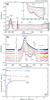 |
Fig. 2 a) Infrared spectra of H2O:CO2 13 K ice (10:1) before (top dark line) and after different irradiation fluences. b) Expanded view from 2200 to 1000 cm-1. c) Molecular column densities derived from the infrared spectra during the experiment. |
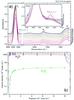 |
Fig. 3 a) Infrared spectra of pure water ice at 13 K obtained for different 52 MeV Ni fluences. Inset figures present details of newly formed species. b) Molecular column densities derived from the infrared spectra during the experiment. |
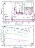 |
Fig. 4 a) Infrared spectra of pure CO2 ice at 13 K after different 52 MeV Ni fluences. Inset figures present details of newly formed species. b) Molecular column densities derived from the infrared spectra during the experiment. |
The infrared spectra of H2O:CO2 (10:1) ice before and after different irradiation fluences up to 5 × 10¹² ions cm-2 are given in Fig. 2a. In contrast to H2O:CO2 (1:1), this ice does not present the OH dangling band at about 3650 cm-1, may come from the lower deposition rate or from the low amount of CO2 on ice. As suggested by Bouwman et al. (2007), the presence of impurities like CO and CO2 on amorphous water ices increases the iceťs porosity and the OH db becomes more prominent.
Figure 2b shows details of the infrared spectra for regions between 2200 to 1000 cm-1. The wavenumber of some unidentified IR frequencies are given. The infrared peaks tentatively attributed to H2CO (~1470 cm-1) and HCOOH (~1220 cm-1) seem to be smaller than for H2O:CO2 (10:1) ice. As in the previous case the appearance of the CO ν1 line at 2139 cm-1 is due to the CO2 radiolysis.
The variations in the column densities of the most abundant molecules observed during the irradiation of H2O:CO2 ice (10:1) by 52 MeV Ni ions as function of fluence are given in Fig. 2c. Peaks due to O3, H2CO3, or CO3 molecules were not observed.
The infrared spectra of pure H2O and CO2 ices at 13 K for different 52 MeV Ni fluences are shown in Figs. 3a and 4a, respectively. Upper curves indicate the virgin ice and figure insets display peak details of the newly formed species. For the radiolysis of pure water, only the formation of H2O2 (vibration mode ν2 + ν6) is observed. In contrast, after the radiolysis of CO2 pure ice, at least three different compounds are formed: CO (ν1), O3 (ν3), and CO3 (ν1) (see also Seperuelo Duarte et al. 2009).
Figure 3b shows the evolution of the water column density derived from different vibration modes (ν1, ν2 and νL) and the column density of H2O2 as a function of ion fluence. The band strengths employed for water vibration modes ν2 (1650 cm-1) was obtained by Gerakines et al. (1995) and νL (~800 cm-1) by Gibb et al. (2000). The evolution of CO2 column density, derived from different vibration modes (ν2, ν3, ν1 + ν3 and 2ν2 + ν3), is given in Fig. 4b: the distinct results are practically the same, as expected. The band strengths employed for CO2 vibration modes ν2 (670 cm-1), 2ν2 + ν3 (3599 cm-1), and ν1 + ν3 (3708 cm-1), were obtained by Gerakines et al. (1995). The column densities of the new species produced by radiolysis are also shown and will be discussed further.
The infrared absorption profile of water (ν1) and carbon dioxide (ν3) in pure and mixed (H2O:CO2 (1:1)) ices as a function of ion fluence are shown in Fig. 5. Upper panels (a and c) indicate pure ices. The selected IR features of mixed ice are illustrated in the bottom panels (b and d). In all panels the upper curves indicate the non-irradiated spectrum. Each spectrum has a small offset for clearer visualization. The bombardment by heavy ions slightly shifts the water ν1 vibration mode to low frequencies. As discussed by Paul et al. (1997), different water clusters are responsible for this IR, therefore this shifts suggests that small water clusters within the ice are being converted to larger cluster structures. Also large clusters may be less radiation sensitive than small clusters. This behavior is enhanced for mixed ices (Fig. 5b).
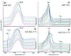 |
Fig. 5 Selected profile of water and CO2 vibration mode at different fluences up to 1013 ions cm-2. Pure water ν1 vibration mode a), water ν1 mode in mixed ices b), pure CO2 ν3 mode c), and CO2 ν3 mode in mixed ices d). See details in text. |
Figure 5b presents the OH dangling bands (~3670 cm-1) attributed to water molecules weakly adsorbed into micropores inside the ice (see Palumbo 2006). As the fluence increases, the micropores collapse and the OH dangling vibration modes decrease. We have shown previously (Pilling et al. 2010) that the ice compaction produced by heavy cosmic rays are at least 3 orders of magnitude higher than what is produced by (0.8 MeV) protons.
The profile of the ν3 vibration mode of carbon dioxide appears to be very sensitive to the presence of water. It becomes very broad and also presents a shift toward the lower frequencies when water is mixed with CO2 (Fig. 5d). As the ion fluence increases, the ν3 band of CO2 becomes sharp and the peak moves toward higher frequencies, becoming similar to pure CO2 ice. A detailed discussion of the effects of CO2 and H2O on band profiles observed in mixed H2O:CO2 ices is given elsewhere (Öberg et al. 2007).
Dissociation cross section, radiochemical yield, and sputtering values of H2O and CO2 obtained from the radiolysis of pure water ice and mixed water-CO2 ices by 52 MeV Ni ions.
4. Discussion
4.1. Dissociation cross section
As discussed previously by Seperuelo Duarte et al. (2009) and Pilling et al. (2010), the complex interaction between an energetic heavy ion with an ice target may be described through partial scenarios by considering successive aspects of the phenomenon. Since the impact of 52 MeV Ni atoms lies in the electronic energy-loss domain (projectile velocity ≳0.01 cm μs-1) most of the deposited energy leads to excitation/ionization of target electrons (electronic energy loss regime). In turn, the electrons liberated from the ion track core (0.3 nm of diameter for 52 MeV Ni atoms; Iza et al. 2006), transfer their energy to the surrounding condensed molecules (~3 nm). The re-neutralization of the track proceeds concomitantly with the local temperature rise, leading to a possible sublimation.
The column density rate (a function of fluence) for each condensed molecular species during radiolysis can be written as 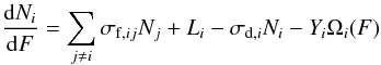 (2)where ∑ jσf,ijNj represents the total molecular production rate of the i species directly from the j species, Li is the layering, σd,i the dissociation cross section, Yi the sputtering yield, and Ωi(F) the relative area occupied by the i species on the ice surface (see details in Pilling et al. 2010).
Considering that the analyzed compounds cannot react in a one-step process to form another species originally present in ice (i.e., σf,ij ≈ 0), for pure ices Eq. (2) can be written by  (3)where N∞,i = (Li − Yi) / σd,i is the asymptotic value of column density at higher fluences owing to the presence of layering, and Ni and N0,i are the column density of species i at a given fluence and at the beginning of experiment, respectively. The layering yield is negligible LCO2 = 0 for pure CO2.
For water-mixed ices, after the rapid ice compaction phase at the beginning of the irradiation, water layering tends to recover the ice surface, Ωi(F) → δi1, progressively preventing the sputtering of CO2 molecules. At the end of these processes, the system of Eq. (2) is decoupled and can be solved analytically by  (4)and
  (5)where N∞ = (L − Y) / σd is the asymptotic value of column density of water because of the presence of layering.
As discussed by Loeffler et al. (2005), the radiochemical formation yield (Gf) of a given compound per 100 eV of deposited energy, at normal incidence, can be expressed in terms of the formation cross section (σf) and the stopping power (S), in units of eV cm2/molec, as 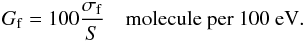 (6)This definition can be extended to the radiochemical dissociation (destruction) yield of a given compound per 100 eV of deposited energy (Gd) by replacing the formation cross section in Eq. (6) by the negative value of the dissociation cross section (−σd). Therefore, negative Gd values indicate that molecules are being dissociated or destroyed after energy deposition into the ice.
By adopting the S values from the stopping and ranges module of the SRIM2003 package (Ziegler 2003), the values of the radiation yield G in the experiments can be determined and compared with the literature values. Table 2 presents the radiochemical destruction yields of H2O and CO2 per 100 eV of deposited energy in each calculated model. The stopping powers of 52 MeV Ni ions for pure water ice and for CO2 ice are S = 1.4 × 10⁻¹² eV cm2/H2O and 2.6 × 10⁻¹² eV cm2/CO2, respectively. For mixed H2O:CO2 ices, the stopping power is determined by interpolation between the pure ice values. We considered that the chemical changes during the irradiation does not affect the stopping power.
Figure 6 presents the fitting curves for the H2O and CO2 column densities employing Eq. (3) for pure ices, and Eqs. (4) and (5) for mixed ices. Numeric labels indicate parameters listed in Table 2. The H2O column density data level off around N∞ ≃ 1.2 × 10¹⁸, 4 × 10¹⁷, and 3 × 10¹⁷ molec cm-2 for pure water, H2O:CO2 (10:1), and H2O:CO2 (1:1) ice samples, respectively. The average value for the dissociation cross section of water, with Eq. (3), is σd ~ 1 × 10-13 cm2. The sputtering yield for water measured by Brown et al. (1984) was extrapolated for the 52 MeV Ni ions’impact as discussed in Pilling et al. (2010). The obtained value is Y = 1 × 10⁴ molec per impact. The estimated average water layering of both experiments was within the 4−14 × 104 molec ion-1 range, obtained from the relation L = N∞σd + Y. The high value of water layering means that CO2 species in the mixed ices were recovered by an H2O film, and the CO2 ice sputtering yield is considered negligible in the current experiments; therefore, the data are adjusted directly by Eq. (5).
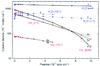 |
Fig. 6 Variation in the experimental column densities of H2O and CO2 as a function of fluence. Lines represent the fittings using Eq. (3) for pure ices and Eqs. (4) and (5) for mixed ices. The parameters models are listed in Table 2. |
The fitting parameters (dissociation cross section, radiochemical yield, sputtering, layering, and the initial relative molecular abundance of each species in the ices) are listed in Table 2. Pure H2O and CO2 ice were fitted by the parameters of models 1 and 4, respectively. For water species the layering yield was determined by L = Ninf + σd + Y. For CO2 species (model 4 to 6b), it is assumed there is no layering due to residual CO2. Model 5a is the fitting for the CO2 species in the mixed H2O:CO2 ice (1:1), and the sputtered value was considered to be half the value from pure CO2 ice.
In model 5b it is assumed that the water layering is high enough to fully cover the CO2 on the surface producing a negligible sputtering yield of CO2 molecules. From the comparison of models 5a and b, we observe that the error in the dissociation cross section is lower than 30%. Model 6a concerns the fitting for the CO2 species in the mixed H2O:CO2 (10:1) ice; the sputtering yield is considered to be a tenth of the value determined for pure CO2 ice.
From models 5, we observe that the sputtering can be precisely determined only for the ices monitored at higher ion fluences (~1013 ion cm-2) since different sets between sputtering and dissociation cross section can be adjusted for the data with low fluences (<5 × 10¹² ions cm-2). Because of the degeneracy of such model for low ion fluence IR data, the error observed in the dissociation cross section on models 6 is about 40%. Table 2 shows that the dissociation cross section at typical astrophysical ice ([CO2]/[H2O] ~ 0.05−0.1) is similar and equal to ~1 × 10-13 cm-2.
4.2. Synthesis of new species
Formation and dissociation cross section of newly formed species from the radiolysis of H2O:CO2 ices by 52 MeV Ni ions.
The evolution of the column density of the newly formed species from H2O:CO2 ices as a function of fluences is shown in Figs. 7a and b. The ratio of H2O2 column density over its parent molecule (H2O) initial column density, NH2O2 / N0,H2O, as a function of fluence in 3 different water-concentration ices (pure H2O ice, ~50% and ~90%) is given in Fig. 7a. The evolution of newly formed species CO, O3, and H2CO3 from CO2-rich ices as a function of fluence is presented in Fig. 7b. The ratio Ni / N0,CO2 indicates the column density ratio of a given produced species over its parent molecule’s (CO2) initial column density. Three different CO2-rich ices are analyzed (pure CO2 ice, ~50% and ~10%). The data was fitted by the simple exponential associate expression: ![Mathematical equation: \begin{equation} N_i/N_{0,p}= A_i + B_i [1- \exp(-\sigma_{{\rm d},i} F)] \label{eq:SigmaForm} \end{equation}](/articles/aa/full_html/2010/15/aa15123-10/aa15123-10-eq103.png) (7)where Ni and N0,p represents the column density of a given produced species i over its parent molecule p (H2O or CO2). Both Ai and Bi are constants that indicate the initial and the maximum amount (after radiolysis) of species i on the ice, σf,i is the formation cross section, and F is the ion fluence.
(7)where Ni and N0,p represents the column density of a given produced species i over its parent molecule p (H2O or CO2). Both Ai and Bi are constants that indicate the initial and the maximum amount (after radiolysis) of species i on the ice, σf,i is the formation cross section, and F is the ion fluence.
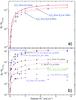 |
Fig. 7 The evolution of newly formed species from the bombardments of H2O:CO2 ices by 52 MeV Ni as a function of fluence. a) Production of H2O2 from H2O molecules in different ices. b) Production of CO, O3, CO3, and H2CO3 from CO2 molecules in different ices. The relative abundance of each parental species is indicated. The lines indicate the fittings using Eq. (11), and the model parameters are given in Table 3. |
As the fluence increases, the number of produced molecules also increases and reaches a maximum. At this moment, the number of molecules produced by radiolysis of parental species is equal to the number of new molecules that possibly dissociate in the reverse reaction set (e.g. p ⇄ i + j + k + ...). At the equilibrium the column density of the parental and daughter species, Neq,p and Neq,i, respectively, are related by the expression:  (8)where σf,i and σd,i is the formation cross section and dissociation cross section of daughter species i.
Since the column densities of daughter species i are much lower than observed for parental species p, as a first approximation we have the following relation between them:  (9)During the whole irradiation time, when a new species is being formed from the radiolysis of its parental species, a fraction of them are also being dissociated and possibly sputtered from the ice. This last effect is not being considered in this model. Since not all the parental molecules are converted into a given species, some could be sputtered from the ice, and others can react to produce different daughter species, the amount of parental molecule always decreases. Consequently, the column density of a given daughter species decreases after it reaches a maximum (equilibrium stage). This behavior can be observed for the evolution of CO3 species as a function of fluence (Fig. 7b).
Calling the maximum amount of newly formed species i at the equilibrium as N∞,i and using Eq. (9), we can express the constant Bi of Eq. (7) by  (10)Moreover, considering that the number of initial daughter species i is negligible (Ai = 0) and, after the combination of Eqs. (9) with (10), we rewrite Eq. (7) as:
 ![Mathematical equation: \begin{equation} N_i/N_{0,p} \simeq \frac{1}{1+\frac{\sigma_{{\rm d},i}}{\sigma_{{\rm f},i}}} [1- \exp(-\sigma_{{\rm d},i} F)] \label{eq:SigmaNEW} \end{equation}](/articles/aa/full_html/2010/15/aa15123-10/aa15123-10-eq118.png) (11)where σd,i and σf,i are the dissociation and formation cross section of species i.
(11)where σd,i and σf,i are the dissociation and formation cross section of species i.
The lines observed in the Figs. 7a and b were obtained by fitting the experimental data with Eq. (11). The proposed model is valid from the beginning of irradiation up to the fluence in which the column density reaches its maximum value. This indicates the equilibrium point between formation and destruction promoted by radiolysis. The formation and dissociation cross sections and the respective radiolysis yield determined for the newly formed species are given in Table 3. We observe that CO presents the highest formation cross section among the newly formed species we studied.
4.2.1. Hydrogen peroxide
In recent years, different groups have studied the formation of hydrogen peroxide (H2O2) by ion bombardment of pure water ice and mixed water-CO2 ices (Moore & Hudson 2000; Strazzulla et al. 2003, 2005a,b; Baragiola et al. 2004; Loeffler et al. 2006; Gomis et al. 2004a,b). H2O2 was also observed from fast electron bombardment of pure water ices (Baragiola et al. 2005; Zheng et al. 2006) and also from low-energy (3−19 eV) electron bombardment (Pan et al. 2004).
Following Teolis et al. (2009), the most commonly H2O2 formation mechanisms involves the reaction between two OH radicals coming from the radiolysis of water molecules, as given by  (12)
(12) (13)where CR denotes cosmic rays.
These OH radicals are strongly hydrogen-bonded to water molecules (Cooper et al. 2003), and it is not until above 80 K that they can diffuse within a water-ice lattice (Johnson & Quickenden 1997). As pointed out by Cooper et al. (2008), energetic OH radicals can diffuse short distances along ion tracks and react at 10 K, but bulk diffusion probably does not occur.
The decrease in the H2O2 production with temperature increase has been investigated by Zheng et al. (2006) and Loeffler et al. (2006). This indicates that electron scavenging may play a critical role in the radiation stability of H2O2 in pure water-ice experiments. Moreover, Gomis et al. (2004a) have found that the H2O2 yields depended on projectile: ices irradiated with low-energy (30 keV) C+, H+, and O+ ions produced more H2O2 at 77 K than 16 K, while N+ and Ar+ had no temperature dependence on the H2O2 yield. The authors have also observed that the H irradiation produces a much lower quantity of H2O2 than for the other heavy ions, suggesting that the energy deposited by elastic collisions plays an important role in this process.
Comparison between the formation and dissociation cross section of H2O2 from the processing of pure H2O ices and H2O:CO2 ices.
As discussed by Zheng et al. (2006) and Loeffler et al. (2006), there is another reaction sequence to produce hydrogen peroxide in astrophysical ices from the addition of oxygen atom (a product of the by the dissociation of oxidant compounds such as O2, CO, CO2, H2O, etc.) to water the molecule:  (14)This reaction route involves an extra ionization stage triggered by CR, UV/X-ray photons, or fast electrons to produce H2O2 (Loeffler et al. 2006), which implies a quadratic dependence on irradiation fluence being a secondary order reaction processes. In the present work we consider the H2O2 formation via oxygen addition to H2O negligible. Future investigations with isotopic labeling could help clarify this issue and quantify which fraction of O atoms produced from the dissociation of CO2 or H2O may react with H2O to form H2O2.
Table 4 presents the formation and dissociation cross section, as well as the radiochemical yield, of H2O2 obtained from the processing of pure water ice and mixed H2O:CO2 ice. Both the formation and dissociation cross section of H2O2 decrease as the relative abundance of H2O in the ice decreases, a consequence of greater averaged distance between parental species. From Fig. 7 we also observe that the presence of CO2 inside the ice decreases the H2O2/H2O ratio. This points in the opposite direction to the results observed from the irradiation of water-CO2 by light ions (Strazzulla et al. 2005b; Moore & Hudson 2000). From Table 4 we observe that the formation cross section of H2O2 from the bombardment of pure water ice by heavy and energetic ions is 105 higher than the value obtained by the impact of light or/and slower projectiles.
The asymptotic value for the H2O2/H2O ratio presents a slight reduction with the enhancement of initial CO2 in the ice. This clearly shows that H2O2 formation via O + H2O, in which the oxygen comes from another oxidant compound, such as CO2, is indeed a second-order process (Loeffler et al. 2006). Our value is about 8 times higher than for irradiation with 30 keV protons, but very similar to the asymptotic values obtained after the impact with other 30 keV ions, such as C+, N+, and O+ (Gomis et al. 2004a). A comparison between our radiochemical yield and cross sections with literature have revealed higher values for both the formation and destruction of H2O2 during bombardments of ices by heavy and energetic ions. In other words, the chemical processing is enhanced by the processing of ices by heavy and energetic and highly charged ions in comparison to light ions.
Hydrogen peroxide has been found on the surface of Europa by identifying both an absorption feature at 3.5 μm in the Galileo NIMS spectra and looking at the UV spectrum taken by the Galileo ultraviolet spectrometer (UVS) (Carlson et al. 1999). Following the authors, the relative abundance with respect to water in Europa is H2O2/H2O ~ 0.001 ( = 0.1%). As the Jupiter satellite is immersed in the intense magnetosphere of the planet, the authors also suggest that radiolysis is the dominant formation mechanism of such a molecule. As discussed by Hendrix et al. (1999), this compound has also been detected on the other icy Galilean moons of Jupiter in the ultraviolet, such as Callisto and Ganymede, although it is less evident on the darker satellites than on Europa. The estimated ratio on Ganymede is H2O2/H2O ~ 0.003 ( = 0.3%) (Hendrix et al. 1999).
Hydrogen peroxide has also been suggested to be present in icy mantles on grains in dense clouds as pointed out Boudin et al. (1998). Based on observations and laboratory studies, they have estimated the relative abundance with respect to water at the dense molecular cloud NGC 7538:IRS 9 of H2O2/H2O ~ 0.05 ( = 5%). Following the authors, hydrogen peroxide can be also produced on grain surfaces via the hydrogenation of molecular oxygen.
4.2.2. Ozone
Ozone (O3) has been detected after irradiation of mixed H2O:CO2 (1:1) ices and pure CO2 ice at 16 K by 1.5−200 keV ions (protons and He+) (Strazzulla et al. 2005a,b). According to these authors, the O3 production from radiolysis is highly attenuated for CO2-poor mixed ices, e.g. for H2O/CO > 2.5. We do not observe ozone among the compounds produced by radiolysis of H2:CO2 (10:1) ice. The presence of ozone is also observed after the irradiation of CO:O2 (1:1) ice by 60 keV Ar++ and 3 keV He+ (Strazzulla et al. 1997). The authors suggest that the detection of ozone and the absence of suboxides (e.g. C2O and C3O) in interstellar grains would indicate a dominance of molecular oxygen in grain mantles. These suboxides have not been detected in our experiments.
Seperuelo Duarte et al. (2010) bombarded pure CO ice with 50 MeV Ni+13 and observed ozone and several suboxides (C2O, C3O2, C5O2) among the radiolysis products. They have determined the ozone formation cross section is 3 × 10-16 cm2. Ozone and suboxides were also observed after irradiation of pure CO ice at 16 K by 200 keV protons (Palumbo et al. 2008).
We detected ozone after the radiolysis of pure CO2 ice and mixed H2O:CO2 (1:1) ice by 52 MeV Ni+13. The determined formation cross section of ozone is σO3 = 0.27 × 10⁻¹³ cm2 in pure CO2 ice and 0.06 × 10⁻¹³ cm2 in H2O:CO2 ice. These values indicate that the O3 formation cross section decreases as the relative abundance of the parental CO2 compound in the ice declines. The value obtained for ozone formation via pure CO2 is 2 times higher than the value determined previously in similar radiolysis experiments involving pure 18CO2 irradiated by 46 MeV 58 Ni+11 (Seperuelo Duarte et al. 2009).
In the solar system, ozone has been observed on Ganymede (Noll et al. 1996) and on Saturn’s satellites Rhea and Dione (Noll et al. 1997). Following Strazzulla et al. (2005a) ozone could be formed where fresh CO2-rich layers are exposed to radiation. The strong silicate absorption band around 1040 cm-1 makes the observation of ozone in interstellar medium very difficult. However, the appearance of ozone seems conceivable, since it is observed in laboratory experiments involving the processing of astrophysical ices analogs.
4.2.3. Carbon trioxide
Carbon trioxide (CO3) has been observed after the UV processing of pure CO2, CO and O2 10 K ices (Gerakines et al. 1996; Gerakines & Moore 2001) and also on radiolysis of pure CO2 by 0.8 MeV protons (Gerakines & Moore 2001) and 1.5 keV protons (Brucato et al. 1997). The bombardment of mixed H2O:CO2 ices by 3 keV He+, 1.5 keV, and 0.8 MeV protons also shows the formation of CO3. Furthermore, H2CO3 and possibly O3 are produced (Brucato et al. 1997; Moore & Khanna 1991).
Seperuelo Duarte et al. (2009) have observed this species in the radiolysis of of C18O2 by 46 MeV 58Ni11+ up to a final fluence of 1.5 × 1013 cm-2. In our measurement the formation cross section of CO3 from radiolysis of pure CO2 ice is 0.08 × 10⁻¹³ cm-2, roughly 5 times lower than the value obtained previously by Seperuelo Duarte et al. (2009). This value presents a decrease in water in the ice, as observed for H2O:CO2 (1:1) ice (see Table 3). The formation cross section of CO in our experiments on pure CO2 is roughly the same as the one determined by Seperuelo Duarte et al. (2009).
The CO3 destruction cross section due to radiolysis is larger than the other compounds formed into the ices. To increase the accuracy of the cross sections, the next measurements should cover large data sets inside the fluence range between 1−10 × 1011 ions cm-2. In contrast to UV photolysis of pure CO2 ices (Gerakines et al. 1996), we do not observe the formation of C3O at 2243 cm-1 from the radiolysis of CO2 ices.
Despite the prediction of CO3 among the compounds in the processed astrophysical ices (e.g. Elsila et al. 1997; Allamandola et al. 1999), this species has not yet been detected conclusively in space (Elsila et al. 1997; Ferrante et al. 2008).
4.2.4. Carbonic acid
Carbonic acid (H2CO3) has been observed in several experiments involving ion bombardment of H2O:CO2 ices (Moore & Khanna 1991; DelloRusso et al. 1993; Brucato et al. 1997). It was also observed after the radiolysis of pure CO2 ice at 10 K by 1.5 keV protons (Brucatto et al. 1997), indicating that implanted hydrogen ions are incorporated in the target to form new bonds to produce H2CO3.
As discussed by Gerakines et al. (2000), the formation of H2CO3 from ion bombardment of H2O:CO2 ices is ruled by two main reaction schemes. First, the direct dissociation of H2O molecules by incoming projectile,  (15)where products such as H2, H2O2; H3O+, and HO2 are eventually formed by reactions involving the primary dissociation products. The next step is the electron attachment to CO2 or OH producing reactive compounds that quickly react with each other to produce bicarbonate (HCO
 ):
):  (16)Finally, bicarbonate reacts with a proton to produce H2CO3:
  (17)From the evolution of the IR peak at 1307 cm-1 during the radiolysis of H2O:CO2 (1:1) ice by 52 MeV Ni ions, we determined the formation and the dissociation cross section of H2CO3 and the values obtained are 3.0 × 10⁻¹⁵ cm2 and 9.9 × 10⁻¹³ cm2, respectively. This formation cross section is 8 orders of magnitude higher than the one derived from the UV photolysis of H2O:CO (1:1) ices at 18 K (Gerakines et al. 2000), indicating that heavy ion processing of astrophysical ice analogs is very efficient to form H2CO3 compared to UV photons.
H2CO3 is thermally stable at 200 K, higher than the sublimation temperature of H2O. As discussed by Peeters et al. (2008), ices containing both H2O and CO2 have been found on a variety of surfaces such as those of Europa, Callisto, Iapetus, and Mars, where processing by magnetospheric ions or the solar wind and energetic solar particles may lead to the formation of H2CO3.
The astrophysical significance of solid carbonic acid has been extensively discussed elsewhere (e.g. Khanna et al. 1994; Brucato et al. 1997; Strazzullla et al. 1996). H2CO3 has been suggested to be present at the surface of several solar system bodies with sufficient amounts of CO2 such as Galilean satellites of Jupiter (Wayne 1995; McCord et al. 1997; Johnson et al. 2004) and comets (Hage et al. 1998). Europa, Ganymede, and Callisto all exhibit high surface CO2 abundances and these satellites are heavily bombarded by energetic magnetospheric particles, galactic cosmic rays, and solar radiation.
It has been suggested that the 3.8 μm feature in NIMS spectra of Ganymede and Callisto arise from H2CO3 (Johnson et al. 2004; Hage et al. 1998). Following Carlson et al. (2005) the relative abundance of carbonic acid with respect to CO2 in Callisto is H2CO3/CO2 ~ 0.01.
The presence of H2CO3 in interstellar ices seems also to be very likely (Whittet et al. 1996) not only in the solid phase but also in gas phase (Hage et al. 1998). For the quiescent cloud medium toward the background field star Elias 16, the expected H2CO3 column density could be as much as 4.6 × 10¹⁶ molec cm-2, corresponding roughly 1% of the CO2 or 0.2% of the total H2O in this line of sight (Whittet et al. 1998).
As discussed by Zheng & Kaiser (2007), in the history of Mars there might be a high concentration of carbonic acid produced by radiolysis of surface H2O:CO2 ices. Without a dense atmosphere and magnetic field, Mars lacks the power to attenuate penetrating energetic solar particles, energetic cosmic rays or any type of high-energy particles. Following Westall et al. (1998), if available in sufficient concentrations, carbonic acid could potentially dissolve metal ores and catalyze chemical reactions, and its presence on Mars may also lead to the existence of limestone (CaCO3), magnesite (MgCO3), dolomite (CaMg(CO3)2), and siderite (FeCO3).
5. Astrophysical implication
Figure 8 presents the total flux of heavy ions (12 ≲ Z ≲ 29) with energy between 0.1−10 MeV/u inside solar system as a function of distance to the Sun. Both Galactic cosmic rays (GCR) and energetic solar particles are displayed. The integrated flux of heavy and energetic solar ions (black square) at Earth Orbit were measured by Mewaldt et al. (2007). Starting from the solar photosphere abundance and the assumption that elements with a first ionization potential of less than 10 eV are more abundant in the energetic solar particles than in the photosphere by a factor of 4.5 (Grevesse et al. 1996) at Earth’s orbit, the integrated flux of heavy and energetic solar particles (φHSW) with energies around 0.1−10 MeV/u was found to be about 1.4 × 10⁻² cm-2 s-1 (black square in Fig. 8).
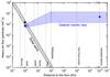 |
Fig. 8 Estimated value of the integrated flux of heavy ions (12 ≲ Z ≲ 29) with energy between 0.1−10 MeV/u inside solar system and at interstellar medium as a function of distance to the Sun. Both Galactic cosmic rays and energetic solar particles are displayed. Square: integrated flux of energetic solar particles. Circle and triangle: integrated flux of cosmic rays. |
The heavy-ion integrated flux at Earth orbit from galactic sources (heavy cosmic rays) was calculated by using the lunar-GCR particle model of Reedy & Arnold (1972) (see also Fig. 3.20 of Vaniman et al. 1991) and taking into account the relative elemental abundances of 12 < Z < 29 atoms at 1 AU (Simpson 1983; Drury et al. 1999). The value obtained was ~7 × 10⁻³ cm-2 s-1 (blue circle in Fig. 8). Assuming that the fluxes of solar wind and energetic solar particles are inversely proportional to the squared distance, this value can be determined as a function of distance up to the heliopause (~100 AU) (i.e. the boundary between the solar wind domain and the interstellar medium).
The average heavy nuclei cosmic ray flux (φHCR) in interstellar medium was estimated by Pilling et al. (2010), who considered the value of φHCR ~ 5 × 10⁻² cm-2 s-1 (blue triangle in Fig. 8). This value was instead the same as at the outer border of heliopause. An error region (dashed area) was introduced in the Fig. 8 to take the uncertainty of these estimations into account.
The value of integrated flux of heavy ions with energies around 0.1−10 MeV/u from galactic sources and energetic solar particles are comparable at the Mars orbit (~1.5 AU). However at the orbits of Jupiter, Saturn, Uranus, and Pluto and at the heliopause border, φHCR/φHSW ~ 2 × 101, 1 × 10², 7 × 10², 3 × 10³ and 2 × 10⁴, respectively. The total flux of heavy particles with energy between 0.1−10 MeV/u at Oort cloud distance was assumed to be the same as expected in the interstellar medium.
Considering the estimated flux of heavy particles of energetic solar particles (φHSW) and of heavy nuclei cosmic rays (φGCR), as well as of the determined dissociation cross section (σd), we can calculate the typical molecular half-lives of frozen molecules in astrophysical surfaces, caused by heavy particles by the expression (see Pilling et al. 2010): ![Mathematical equation: \begin{equation} t_{1/2} \approx \frac{\ln 2}{(\phi_{HSW} + \phi_{HCR}) \times \sigma_{\rm d}} \quad {\rm [s^{-1}].} \end{equation}](/articles/aa/full_html/2010/15/aa15123-10/aa15123-10-eq163.png) (18)
(18)
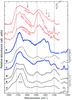 |
Fig. 9 Comparison between IR spectra of interstellar and laboratory ices. The top three curves are infrared spectra of young stellar sources obtained by the Infrared Space Observatory (ISO). Lower traces indicate different laboratory spectra of irradiated H2O:CO2 ices: a) and c) (this work); b) (Hudson & Moore 2001); d) (Gerakines et al. 2000); e) (Strazzulla et al. 2005b); f) (UV photons, Gerakines et al. 2000). Vertical dashed lines indicate the location of vibrational modes of frozen H2CO3. |
It is worth noting that the present experiments were performed at the low temperature of 13 K, the temperature that is adequate for ices in the interstellar medium. Therefore it is useful to compare IR spectra of interstellar and laboratory ices as shown in Fig. 9. The IR spectra of young stellar sources (top tree curves) were obtained by the Infrared Space Observatory (ISO). The six bottom curves indicate different laboratory spectra of processed H2O:CO2 ices: a) mixture (10:1) irradiated by 52 MeV Ni ions (this work); b) mixture (10:1) irradiated by 0.8 MeV protons (Hudson & Moore 2001); c) mixture (1:1) irradiated by 52 MeV Ni ions (this work); d) mixture (1:1) irradiated by 0.8 MeV protons (Gerakines et al. 2000); e) mixture (1:1) irradiated by 0.8 MeV protons (Strazzulla et al. 2005b); and f) mixture (1:1) irradiated by UV photons (Gerakines et al. 2000). Our data are represented by two bold (blue) curves. The location of vibrational modes of frozen H2CO3 (Moore & Khanna 1991) is indicated. The presence of H2CO3 seems to be independent of the ionization source.
The three bumps observed on the IR spectra of the young stelar objects at about 1600 cm-1, 1400 cm-1, and 1350 cm-1 (see arrows in Fig 9) present a good similarity with the features present in the IR spectra of H2O:CO2 (10:1) irradiated by 52 MeV ions (curve a). Nevertheless, up to now, its molecular assignment remains unknown. Although very attenuated, these features are still observed in the IR spectra of H2O:CO2 (1:1) (curve c). This suggests that heavy cosmic rays can be good candidates for explaining some features observed in the IR spectra of some interstellar sources.
The comparison between the current results with the previous one (Pilling et al. 2010) reveals that, independent of ice constitution (involving H2O, CO2, CO, and NH3), the dissociation cross section due to heavy and energetic cosmic ray analogs are in the same range, σd = 1−2 × 10-13 cm2. This supports the extension of our previous estimative for the half-life of ammonia-containing ice, τ1 / 2 = 2−3 × 10⁶ years, to all kinds of interstellar grains inside dense interstellar environments in the presence of a constant galactic heavy cosmic ray flux.
The temperature of solar system ices is about 80 K, a value about 5−8 times higher than observed in interstellar ices; therefore, some molecular species (the most volatile as O3 and CO) are not efficiently trapped/adsorbed in/on the ices. This can make an enormous difference in surface and bulk chemistry. Future experiments employing H2O:CO2 ices at 80 K will be performed to investigate this question.
6. Summary and conclusions
The interaction of heavy, highly charged, and energetic ions (52 MeV 58Ni13+) with pure H2O and CO2 ices and mixed (H2O:CO2) ices was studied experimentally. The aim was to understand the chemical and the physicochemical processes induced by heavy cosmic rays inside dense and cool astrophysical environments, such as molecular clouds and protostellar clouds, as well on the surfaces solar system ices. Our main results and conclusions are the following.
-
1.
In all experiments containing CO2 (pure ice and mixtures) after a fluence of about 2−3 × 10¹² ions cm-2, the CO2/CO ratio became roughly constant (~0.1), independent of initial CO2/H2O. The experiments suggest that the abundances of CO3, O3, and H2CO3 in typical astrophysical ices ([CO2]/[H2O] ~ 0.05−0.1) irradiated by heavy ions, should be very low, except for those ices with peculiar enrichment of CO2.
-
2.
After a fluence of about 2−3 × 10¹² ions cm-2, the H2O2/H2O ratio stabilizes at ~0.01, is independent of initial H2O relative abundance and column density.
-
3.
A comparison between our radiochemical yields and cross sections with the literature have revealed higher values for both the formation and destruction of H2O2 during bombardments of ices by heavy and energetic ions. In other words, the chemical processing is enhanced by the processing of ices by heavy and energetic and highly charged ions in comparison to light ions.
-
4.
The dissociation cross section of pure H2O and CO2 ices are 1.1 and 1.9 × 10⁻¹³ cm2, respectively. For mixed H2O:CO2 (10:1) ice, the dissociation cross section of both species is roughly 1 × 10-13 cm2.
-
5.
Some IR features observed in ices after the bombardment by heavy ions present a strong similarity with those observed at molecular clouds, suggesting that heavy cosmic rays play an important role in the processing of frozen compounds in interstellar environments.
Acknowledgments
The authors acknowledge the agencies COFECUB (France), CAPES, CNPq, and FAPERJ (Brazil) for financial support. We thank Th. Been, I. Monnet, Y. Ngono-Ravache, and J.M. Ramillon for technical support.
References
- Allamandola, L. J., Bernstein, M. P., Sandford, S. A., & Walker, R. L. 1999, Space Sci. Rev., 90, 219 [NASA ADS] [CrossRef] [PubMed] [Google Scholar]
- Baragiola, R. A., Loeffler, M. J., Raut, U., Vidal, R. A., & Carlson, R. W. 2004, Lunar and Planetary Science Conference, 35, 2079 [Google Scholar]
- Baragiola, R. L. A., Loeffler, M. J., Raut, U., Vidal, R. A., & Wilson, C. D. 2005, Radiat. Phys. Chem., 72, 187 [NASA ADS] [CrossRef] [Google Scholar]
- Bennett, C. J., Jamieson, C. S., Mebel, A. M., & Kaiser, R. I. 2004, Phys. Chem. Chem. Phys., 6, 735 [CrossRef] [Google Scholar]
- Bockelée-Morvan, D. 1997, in Molecules in Astrophysics: Probes and Processes, ed. E. F. van Dishoeck (Dordrecht: Kluwer), 218 [Google Scholar]
- Boudin, N., Schutte, W. A., & Greenberg, J. M. 1998, A&A, 331, 749 [NASA ADS] [Google Scholar]
- Bouwman, J., Ludwig, W., Awad, Z., et al. 2007, A&A, 476, 995 [NASA ADS] [CrossRef] [EDP Sciences] [Google Scholar]
- Brown, W. L., Augustyniak, W. M., Marcantonio, K. J., et al. 1984, Nucl. Instr. and Meth. B1, IV, 307 [NASA ADS] [CrossRef] [Google Scholar]
- Brucato, J. R., Palumbo, M. E., & Strazzulla, G. 1997, Icarus, 125, 135 [NASA ADS] [CrossRef] [Google Scholar]
- Carlson, R. W., Anderson, M. S., Johnson, R. E., et al. 1999, Science, 283, 2062 [NASA ADS] [CrossRef] [PubMed] [Google Scholar]
- Carlson, R. W., Hand, K. P., Gerakines, P. A., Moore, M. H., & Hudson, R. L. 2005, BAAS, 37, 5805 [Google Scholar]
- Cooper, P. D., Johnson, R. E., & Quickenden, T. I. 2003, Icarus, 166, 444 [NASA ADS] [CrossRef] [Google Scholar]
- Cooper, P. D., Moore, M. H., Hudson, R. L., et al. 2008, Icaurs, 194, 379 [Google Scholar]
- Crovisier, J. 1998, Faraday Discuss., 109, 437 [NASA ADS] [CrossRef] [Google Scholar]
- Crovisier, J., Leech, K., Bockelee-Morvan, D., et al. 1997, Science, 275, 1904 [CrossRef] [Google Scholar]
- DelloRusso, N., Khanna, R. K., & Moore, M. H. 1993, JGR, 98, 5505 [NASA ADS] [CrossRef] [Google Scholar]
- Drury, L. O. C., Meyer, J.-P., & Ellison, D. C. 1999, Topics in Cosmic-Ray Astrophysics, ed. M. A. DuVernois (New-York: Nova Science Publishers) [Google Scholar]
- Ehrenfreund, P., & Charnley, S. B. 2000, ARA&A, 38, 427 [Google Scholar]
- Elsila, J., Allamandola, L. J., & Sandford, S. A. 1997, ApJ, 479, 818 [NASA ADS] [CrossRef] [PubMed] [Google Scholar]
- Ferrante, R. F., Moore, M. H., Morgan, M., Spiliotis, M. M., & Hudson, R. L. 2008, ApJ, 684, 1210 [NASA ADS] [CrossRef] [Google Scholar]
- Gerakines, P. A., & Moore, M. H. 2001, Icarus, 154, 372 [NASA ADS] [CrossRef] [Google Scholar]
- Gerakines, P. A., Scutte, W. A., Greenberg, J. M., & van Dishoeck, E. F. 1995, A&A, 296, 810 [NASA ADS] [Google Scholar]
- Gerakines, P. A., Schutte, W. A., & Ehrenfreund, P. 1996, A&A, 312, 289 [NASA ADS] [Google Scholar]
- Gerakines, P. A., Whittet, D. C. B., Ehrenfreund, P., et al. 1999, ApJ, 522, 357 [NASA ADS] [CrossRef] [Google Scholar]
- Gerakines, P. A., Moore, M. H., & Hudson, R. L. 2000, A&A, 357, 793 [NASA ADS] [Google Scholar]
- Gibb, E. L., Whittet, D. C. B., Schutte, W. A., et al. 2000, ApJ, 536, 347 [NASA ADS] [CrossRef] [Google Scholar]
- Gomis, O., Satorre, M. A., Strazzulla, G., & Leto, G. 2004a, PSS, 52, 371 [Google Scholar]
- Gomis, O., Leto, G., & Strazzulla, G. 2004b, A&A, 420, 405 [NASA ADS] [CrossRef] [EDP Sciences] [Google Scholar]
- Grevesse, N., Noels, A., & Sauval, J. A. 1996, ASP Conf. Ser., 99, 117 [NASA ADS] [Google Scholar]
- Hage, W., Liedl, K. R., Hallbrucker, A., & Mayer, E. 1998, Science, 279, 1332 [CrossRef] [Google Scholar]
- d’Hendecourt, L. B., & Allamandola, L. J. 1986, A&AS, 64, 453 [NASA ADS] [Google Scholar]
- Hendrix, A. R., Barth, C. A., Stewart, A. I. F., Hord, C. W., & Lane, A. L. 1999, LPI, 30, 2043 [NASA ADS] [Google Scholar]
- Herr, K. C., & Pimentel, G. C. 1969, Science, 166, 496 [NASA ADS] [CrossRef] [PubMed] [Google Scholar]
- Hudson, R. L., & Moore, M. H. 2001, J. Geoph. Res., 106, 33275 [NASA ADS] [CrossRef] [Google Scholar]
- Iza, P., Farenzena, L. S., Jalowy, T., Groeneveld, K. O., & da Silveira, E. F. 2006, Nucl. Instr. Meth. Phys. Res., Sect. B, 245, 61 [Google Scholar]
- Johnson, R. E., & Quickenden, T. I. 1997, JGR, 102, 10985J [NASA ADS] [CrossRef] [Google Scholar]
- Johnson, R. E., Carlson, R. W., Cooper, J. F., et al. 2004, in Jupiter: The planet, satellites and magnetosphere, ed. F. Bagenal, T. E. Dowling, & W. B. McKinnon, Cambridge Planetary Science, vol. 1 (Cambridge, UK: Cambridge University Press), 485 [Google Scholar]
- Khanna, R. K., Tossell, J. A., & Fox, F. 1994, Icarus, 112, 541 [NASA ADS] [CrossRef] [Google Scholar]
- Larson, H. P., & Fink, U. 1972, ApJ, 171, L91 [NASA ADS] [CrossRef] [Google Scholar]
- Leto, G., & Baratta, G. A. 2003, A&A, 397, 7 [Google Scholar]
- Loeffler, M. J., Barata, G. A., Palumbo, M. E., Strazulla, G., & Baragiola, R. A. 2005, A&A, 435, 587 [NASA ADS] [CrossRef] [EDP Sciences] [MathSciNet] [Google Scholar]
- Loeffler, M. J., Raut, U., Vidal, R. A., Baragiola, R. A., & Carlson, R. W. 2006, Icarus, 180, 265 [NASA ADS] [CrossRef] [Google Scholar]
- McCord, T. B., Carlson, R., Smythe, W., et al. 1997, Science, 278, 271 [NASA ADS] [CrossRef] [PubMed] [Google Scholar]
- McCord, T. B., Hansen, G. B., Clark, R. N., et al. 1998, J. Geophys. Res., 103, 8603 [NASA ADS] [CrossRef] [Google Scholar]
- Moore, M., & Hudson, R. L. 2000, Icarus, 145, 282 [NASA ADS] [CrossRef] [Google Scholar]
- Moore, M. H., & Khanna, R. K. 1991, Spectrochim. Acta, 47, 255 [CrossRef] [Google Scholar]
- Mewaldt, R. A., Cohen, C. M. S., Mason, G. M., Haggerty, D. K., & Desai, M. I. 2007, Space Sci. Rev., 130, 323 [NASA ADS] [CrossRef] [Google Scholar]
- Nastasi, M., Mayer, J., & Hirvonen, J. K. 1996, in Ion-Solid Interactions: Fundamentals and Applications, Cambridge Solid State Science Series (Cambridge University Press) [Google Scholar]
- Noll, K. S., Johnson, R. E., Lane, A. L., Domingue, D. L., & Weaver, H. A. 1996, Science, 273, 341 [NASA ADS] [CrossRef] [PubMed] [Google Scholar]
- Noll, K. S., Roush, T. L., Cruikshank, D. P., Johnson, R. E., & Pendleton, Y. J. 1997, Nature, 388, 45 [NASA ADS] [CrossRef] [Google Scholar]
- Öberg, K. I., Fraser, H. J., Boogert, A. C. A., et al. 2007, A&A, 462, 1187 [NASA ADS] [CrossRef] [EDP Sciences] [Google Scholar]
- Pan, X. N., Bass, A. D., Jay-Gerin, J. P., & Sanche, L. 2004, Icarus, 172, 521 [NASA ADS] [CrossRef] [Google Scholar]
- Palumbo, M. E. 2006, A&A, 453, 903 [NASA ADS] [CrossRef] [EDP Sciences] [MathSciNet] [Google Scholar]
- Palumbo, M. E., Baratta, G. A., & Spinella, F. 2006, Mem. S.A.It. Suppl., 9, 192 [Google Scholar]
- Palumbo, M. E., Leto, P., Siringo, C., & Trigilio, C. 2008, ApJ, 685, 1033 [NASA ADS] [CrossRef] [Google Scholar]
- Paul, J. B., Collier, C. P., Saykally, R. J., Scherer, J. J., & O’Keefe, A. 1997, J. Phys. Chem. A, 101, 5211 [CrossRef] [Google Scholar]
- Peeters, Z., Hudson, R., & Moore, M. 2008, DPS, 40, 5405 [NASA ADS] [Google Scholar]
- Pilling, S., Seperuelo Duarte, E., da Silveira, E. F., et al. 2010, A&A, 509, A87 [NASA ADS] [CrossRef] [EDP Sciences] [Google Scholar]
- Quirico, E., Douté, S., Schmitt, B., et al. 1999, Icarus, 139, 159 [NASA ADS] [CrossRef] [Google Scholar]
- Reedy, R. C., & Arnold, J. R. 1972, J. Geophys. Res., 77, 537 [NASA ADS] [CrossRef] [Google Scholar]
- Seperuelo Duarte, E., Boduch, P., Rothard, H., et al. 2009, A&A, 502, 599 [NASA ADS] [CrossRef] [EDP Sciences] [Google Scholar]
- Seperuelo Duarte, E., Domaracka, A., Boduch, P., et al. 2010, A&A, 512, A71 [NASA ADS] [CrossRef] [EDP Sciences] [Google Scholar]
- Simpson, J. A. 1983, Ann. Rev. Nucl. Part. Sci., 33, 323 [Google Scholar]
- Smith, M. A. H., Rinsland, C. P., Fridovich, B., & Rao, K. N. 1985, in Molecular Spectroscopy: Modern Research (London: Academic), 3 [Google Scholar]
- Strazzullla, G., Brucato, J. R., Cimino, G., & Palumbo, M. E. 1996, Planet. Space Sci., 44, 1447 [Google Scholar]
- Strazzulla, G., Brucato, J. R., Palumbo, M. E., & Satorre, M. A. 1997, A&A, 321, 618 [NASA ADS] [Google Scholar]
- Strazzulla, G., Leto, G., Gomis, O., & Satorre, M. A. 2003, Icarus, 164, 163 [NASA ADS] [CrossRef] [Google Scholar]
- Strazzulla, G., Leto, G., Spinella, F., & Gomis, O. 2005a, Astrobiology, 5, 612 [NASA ADS] [CrossRef] [PubMed] [Google Scholar]
- Strazzulla, G., Leto, G., Spinella, F., & Gomis, O. 2005b, Mem. S.A.It. Suppl., 6, 51 [Google Scholar]
- Teolis, B. D., Shi, J., & Baragiola, R. A. 2009, JCP, 130, 134704 [CrossRef] [Google Scholar]
- Wayne, R. P. 1995, Chemistry of the Atmospheres, Chaps. 8 and 9 (Oxford: Clarendon Press) [Google Scholar]
- Westall, F., Gobbi, P., Gerneke, D., & Mazzotti, G. 1998, in Lunar and Planetary Institute Conference Abstracts, 1362 [Google Scholar]
- Whittet, D. C. B., Schutte, W. A., Tielens, A. G. G. M., et al. 1996, A&A, 315, L357 [NASA ADS] [Google Scholar]
- Whittet, D. C. B., Gerakines, P. A., Tielens, A. G. G. M., et al. 1998, ApJ, 498, L159 [NASA ADS] [CrossRef] [Google Scholar]
- Wu, C. Y. R., et al. 2003, J. Geophys. Res., 108(E4), 13-1 [Google Scholar]
- Vaniman, D., Reedy, R., Heiken, G., Olhoeft, G., & Mendell, W. 1991, in Lunar Sourcebook: a user’s guide to the Moon, ed. G. H. Heiken, D. T. Vaniman, & B. M. French (Cambridge Univ. Press), 55 [Google Scholar]
- Zheng, W., & Kaiser, R. I. 2007, Chem. Phys. Lett., 450, 55 [NASA ADS] [CrossRef] [Google Scholar]
- Zheng, W., Jewitt, D., & Kaiser, R. 2006, ApJ, 639, 534 [NASA ADS] [CrossRef] [Google Scholar]
- Ziegler, J. F. 2003, Stopping and Range of Ions in Matter SRIM2003 (available at www.srim.org) [Google Scholar]
All Tables
Infrared absorption coefficients (band strengths) used in the column density calculations for the observed molecules.
Dissociation cross section, radiochemical yield, and sputtering values of H2O and CO2 obtained from the radiolysis of pure water ice and mixed water-CO2 ices by 52 MeV Ni ions.
Formation and dissociation cross section of newly formed species from the radiolysis of H2O:CO2 ices by 52 MeV Ni ions.
Comparison between the formation and dissociation cross section of H2O2 from the processing of pure H2O ices and H2O:CO2 ices.
All Figures
|
Fig. 1 a) Infrared spectra of H2O:CO2 13 K ice (1:1) before (top dark line) and after different irradiation fluences. b) Expanded view from 2200 to 1000 cm-1. c) Molecular column densities derived from the infrared spectra during the experiment. The lines are added to guide the eyes. |
| In the text | |
|
Fig. 2 a) Infrared spectra of H2O:CO2 13 K ice (10:1) before (top dark line) and after different irradiation fluences. b) Expanded view from 2200 to 1000 cm-1. c) Molecular column densities derived from the infrared spectra during the experiment. |
| In the text | |
|
Fig. 3 a) Infrared spectra of pure water ice at 13 K obtained for different 52 MeV Ni fluences. Inset figures present details of newly formed species. b) Molecular column densities derived from the infrared spectra during the experiment. |
| In the text | |
|
Fig. 4 a) Infrared spectra of pure CO2 ice at 13 K after different 52 MeV Ni fluences. Inset figures present details of newly formed species. b) Molecular column densities derived from the infrared spectra during the experiment. |
| In the text | |
|
Fig. 5 Selected profile of water and CO2 vibration mode at different fluences up to 1013 ions cm-2. Pure water ν1 vibration mode a), water ν1 mode in mixed ices b), pure CO2 ν3 mode c), and CO2 ν3 mode in mixed ices d). See details in text. |
| In the text | |
|
Fig. 6 Variation in the experimental column densities of H2O and CO2 as a function of fluence. Lines represent the fittings using Eq. (3) for pure ices and Eqs. (4) and (5) for mixed ices. The parameters models are listed in Table 2. |
| In the text | |
|
Fig. 7 The evolution of newly formed species from the bombardments of H2O:CO2 ices by 52 MeV Ni as a function of fluence. a) Production of H2O2 from H2O molecules in different ices. b) Production of CO, O3, CO3, and H2CO3 from CO2 molecules in different ices. The relative abundance of each parental species is indicated. The lines indicate the fittings using Eq. (11), and the model parameters are given in Table 3. |
| In the text | |
|
Fig. 8 Estimated value of the integrated flux of heavy ions (12 ≲ Z ≲ 29) with energy between 0.1−10 MeV/u inside solar system and at interstellar medium as a function of distance to the Sun. Both Galactic cosmic rays and energetic solar particles are displayed. Square: integrated flux of energetic solar particles. Circle and triangle: integrated flux of cosmic rays. |
| In the text | |
|
Fig. 9 Comparison between IR spectra of interstellar and laboratory ices. The top three curves are infrared spectra of young stellar sources obtained by the Infrared Space Observatory (ISO). Lower traces indicate different laboratory spectra of irradiated H2O:CO2 ices: a) and c) (this work); b) (Hudson & Moore 2001); d) (Gerakines et al. 2000); e) (Strazzulla et al. 2005b); f) (UV photons, Gerakines et al. 2000). Vertical dashed lines indicate the location of vibrational modes of frozen H2CO3. |
| In the text | |
Current usage metrics show cumulative count of Article Views (full-text article views including HTML views, PDF and ePub downloads, according to the available data) and Abstracts Views on Vision4Press platform.
Data correspond to usage on the plateform after 2015. The current usage metrics is available 48-96 hours after online publication and is updated daily on week days.
Initial download of the metrics may take a while.