| Issue |
A&A
Volume 523, November-December 2010
|
|
|---|---|---|
| Article Number | A47 | |
| Number of page(s) | 12 | |
| Section | The Sun | |
| DOI | https://doi.org/10.1051/0004-6361/201014261 | |
| Published online | 16 November 2010 | |
Radiative and magnetic properties of solar active regions
II. Spatially resolved analysis of O V 62.97 nm transition region emission
1
Space Science and Technology DepartmentSTFC Rutherford Appleton
Laboratory, Chilton, Didcot
OX11 0QX, UK
e-mail: This email address is being protected from spambots. You need JavaScript enabled to view it.
2
Space Science Division, Naval Research Laboratory,
Washington, DC
20375,
USA
e-mail: This email address is being protected from spambots. You need JavaScript enabled to view it.
Received:
15
February
2010
Accepted:
11
August
2010
Abstract
Context. Global relationships between the photospheric magnetic flux and the extreme ultraviolet emission integrated over active region area have been studied in a previous paper by Fludra & Ireland (2008, A&A, 483, 609). Spatially integrated EUV line intensities are tightly correlated with the total unsigned magnetic flux, and yet these global power laws have been shown to be insufficient for accurately determining the coronal heating mechanism owing to the mathematical ill-conditioning of the inverse problem.
Aims. Our aim is to establish a relationship between the EUV line intensities and the photospheric magnetic flux density on small spatial scales in active regions and investigate whether it provides a way of identifying the process that heats the coronal loops.
Methods. We compare spatially resolved EUV transition region emission and the photospheric magnetic flux density. This analysis is based on the O V 62.97 nm line recorded by the SOHO Coronal Diagnostic Spectrometer (CDS) and SOHO MDI magnetograms for six solar active regions. The magnetic flux density φ is converted to a simulated O V intensity using a model relationship I(φ,L) = CφδLλ, where the loop length L is obtained from potential magnetic field extrapolations. This simulated spatial distribution of O V intensities is convolved with the CDS instrument’s point spread function and compared pixel by pixel with the observed O V line intensity. Parameters δ and λ are derived to give the best fit for the observed and simulated intensities.
Results. Spatially-resolved analysis of the transition region emission reveals the complex nature of the heating processes in active regions. In some active regions, particularly large, local intensity enhancements up to a factor of five are present. When areas with O V intensities above 3000 erg cm-2 s-1 sr-1 are ignored, a power law has been fitted to the relationship between the local O V line intensity and the photospheric magnetic flux density in each active region. The average power index δ from all regions is 0.4 ± 0.1 and λ = − 0.15 ± 0.07. However, the scatter of intensities in all regions is significantly greater than ± 3σ from the fitted model. We therefore determine for the first time an empirical lower boundary for the IOV − φ relationship that is the same for five active regions. We postulate that it represents a basal heating. Because this boundary is present in the spatially-resolved data, this is compelling proof that the magnetic field is one of the major factors contributing to the basal component of the heating of the coronal plasma. We discuss the implications for the diagnostics of the coronal heating mechanism.
Key words: Sun: UV radiation / Sun: surface magnetism / Sun: transition region / Sun: corona / magnetic fields
© ESO, 2010
1. Introduction
The hot plasmas in the solar corona and transition region emit radiation at X-ray and extreme ultraviolet (EUV) wavelengths, which can then be used to diagnose the conditions of the plasma. The question of what heats the coronal plasma to temperatures from 20 000 K to several million K has been pursued for the past three decades. One of the approaches to the search for the coronal heating mechanism has been to study the relationships between the X-ray and EUV line emission and the photospheric magnetic field in solar active regions. Past research has shown that the total intensity of EUV spectral lines and a broad-band X-ray flux summed over an entire active region are related to the global magnetic quantities (e.g., Fisher et al. 1998; Pevtsov et al. 2003; Fludra & Ireland 2008).
The expectation of such analysis was that these well-defined relationships could be compared to theoretical predictions from the many models of coronal heating and provide constraints to identify the correct model. The attractiveness of the global power laws extending sometimes over several orders of magnitude led many researchers into believing that these power laws offer a direct recipe for deriving the heating mechanism. However, such conjectures were only qualitative and largely unsubstantiated.
List of active regions.
Fludra & Ireland (2008) presented for the first time a detailed analysis of the diagnostic capability of the power index, α, in the global relationship, IT = CΦα, where Φ is the total unsigned magnetic flux in the active region. They have exposed limitations of the global analysis and shown that the inverse problem of deriving the I − φ relationship between the emission from a single loop and the magnetic flux density, φ, at its footpoint, from the global IT − Φ relationship is mathematically ill-conditioned, particularly for the transition region lines, where α < 1.
Despite the shortcomings and uncertainties inherent in the global analysis, they were able to estimate that, under the assumption of hydrostatic equilibrium, the power index γ characterising the volumetric heating rate EH ∝ φγ lies in a broad but still useful range of 0.6 < γ < 1.1.
A novel extension of the global analysis was proposed by Fludra & Ireland (2003) who replaced the total unsigned magnetic flux with spatially resolved magnetic flux density while keeping the spatially integrated EUV line intensities. This resulted in an integral equation that had the form of a Laplace transform and could be analytically inverted to obtain the dependence of intensity in individual coronal loops on the magnetic flux density at their footpoints.
In this paper we study a third approach, which uses both spatially resolved EUV intensities and spatially resolved magnetic flux density. This was attempted by Aschwanden et al. (1999) to compare active region coronal loops with the photospheric magnetic flux at their footpoints, a task made difficult by the need to project a coronal loop precisely to the photospheric level. It would appear that such spatially resolved comparisons would be easier for the transition region emission, which often is expected to be located above the loop footpoints. Fludra & Ireland (2004) did such preliminary analysis for a few active regions observed by the SOHO Coronal Diagnostic Spectrometer (CDS). That such comparisons have not been done for the CDS observations before was due to a technical problem of a precise co-alignment between pixels of rastered images obtained with a spectrometer and magnetograms (see Sect. 2.1). Here we expand and refine the work of Fludra & Ireland (2004), including the loop lengths obtained from magnetic field extrapolations, and discuss the diagnostic capability of the combined EUV and magnetic data to determine the heating rate dependence on the magnetic flux density.
Studies of the transition region have received considerable attention since the launch of SOHO, to characterise and understand the dynamic behaviour and variability of the transition region emission both in the quiet sun and active regions (e.g., Fludra et al. 1997; Harrison et al. 1999; Fludra 1999, 2001; Parnell et al. 2002; Jordan et al. 2005). Data from the SOHO Coronal Diagnostic Spectrometer (Harrison et al. 1995) have played a significant role in these investigations, providing measurements of several strong spectral lines, including He I 58.43 nm and O V 62.97 nm. Spectral line profiles are useful for measuring velocity and intensity oscillations in the quiet sun and active regions, random intensity fluctuations (brightening events), flow velocities and their statistical properties. To determine the mechanism responsible for intensity bursts, however, line intensities need to be compared to the underlying photospheric magnetic field. Such comparisons have been rare, e.g., Tarbell et al. (1999) showed the spatial and temporal correspondence of O V intensity fluctuations with the magnetic dipole cancellation.
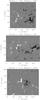 |
Fig. 1 MDI magnetograms for active regions 1 (top), 2 (middle) and 3 (bottom) from Table 1. Contours correspond to absolute magnetic flux density of 90 Mx cm-2. Bmax,b and Bmax,w are maximum values (Mx cm-2) of the negative (black) and positive (white) polarity, respectively. |
In this paper, we carry out a detailed comparison between the transition region emission and the magnetic field in active regions. We address the following questions: (a) what is the relationship between the intensities of the O V 62.97 nm line and the photospheric magnetic field on small spatial scales of a few arcseconds. Is this relationship as well defined as it is for the global, spatially integrated quantities? (b) Is it the same in different active regions? (c) can the transition region emission be used to study the heating mechanism in active regions; (d) can the EUV emission in coronal loops be predicted from the magnetic field at the loop footpoints? Section 2 describes the data and analysis procedures. Results are discussed in Sect. 3.
2. Data analysis
The wavelength range of CDS covers lines emitted at temperatures from the low transition region at 3 × 10⁴ K to the hottest parts of active coronal loops at several million degrees. A full description of the CDS is given by Harrison et al. (1995) and application to active region observations is shown by Fludra et al. (1997). The data discussed in this paper were recorded by the Normal Incidence Spectrometer using a 2 × 240 arcsec slit. At each slit position, an exposure of 15 s duration was taken and four wavelength windows, centred on selected spectral lines were extracted and transmitted: He I 58.43, O V 62.97, Mg IX 36.81, Fe XVI 36.08 nm. The width of the spectral windows was sufficient to include the full line profile and adjacent background.
After each exposure, the scanning mirror is rotated by one step, equivalent to the width of the slit, so that the adjacent area of the Sun is presented to the slit, another exposure is taken, the mirror is rotated again, and so on, until the whole required area of the Sun is covered. A maximum area that can be covered by the CDS raster without repointing the instrument is 4 × 4 arcmin2. The spatial dimensions of the raster elements (pixels) are 2 arcsec in the EW direction and 1.68 arcsec in the N S direction.
We select six regions observed by the CDS synoptic data taken between February 1997 and June 1998 (Table 1). Four of the synoptic spectral lines (He I, O V, Mg IX, and Fe XVI) were previously analysed in the study of global relationships, IT − Φ, by Fludra & Ireland (2008). The Fe XVI 36.08 nm line was analysed separately by Fludra & Ireland (2003), to illustrate the application of their new inverse method to the IT − Φ relationship. In this paper, we analyse only the transition region line O V 62.97 nm, using CDS rastered images (2′′ × 1.68′′ pixels) and comparing them to SOHO MDI magnetograms (Scherrer et al. 1995) with 2′′ × 2′′ pixels.
The CDS raster pointing is known with an uncertainty of approximately up to ± 6′′. As we require a co-alignment between the CDS rasters and MDI magnetic field comparable to the size of the CDS and MDI pixels (2′′), this is achieved by cross-correlating individual CDS rasters with MDI (see Sect. 2.1). We restrict the present study to active regions that fully fit into the 4′ × 4′ area of one CDS raster – this minimises the time taken to obtain a CDS map of the active region and minimises co-alignment errors between CDS and MDI.
The magnetic flux density is taken from full disk line-of-sight magnetograms recorded by the MDI instrument on SOHO with a 2′′ × 2′′ spatial resolution. These magnetograms are taken every 96 min, therefore, they do not coincide exactly with the time of CDS rasters. We choose the magnetogram closest in time to the start of the CDS raster. We use magnetograms with the latest calibration available from December 2008.
Additionally, the magnetic flux density has been corrected for the line of sight projection. Assuming a radial magnetic field, the correction factor depends on the latitude and longitude.
Within a box enclosing the EUV emission of the active region, the magnetograms contain both low values of the magnetic flux density characteristic of the quiet sun, and high values characteristic of active regions. We define the active region magnetic area by using a fixed threshold of Bth = 90 Mx cm-2 (Fludra & Ireland 2008). For old, uncalibrated MDI data available in 1996–2007 this corresponds to a threshold of approximately 50 Mx cm-2. Figures 1 and 2 show SOHO/MDI magnetograms for the six regions analysed in this paper, where the displayed area is the same as the analysed CDS field of view. Contours in Figs. 1 and 2 correspond to the absolute value of the magnetic flux density of 90 Mx cm-2. The histograms of the magnetic flux density inside the contours, when binned with a step of 10 Mx cm-2, are approximately exponential. An example histogram is shown by Fludra & Ireland (2008, their Fig. 2). Maximum values of the absolute magnetic flux density in each region, Bmax, are listed in Table 1.
2.1. Comparison of spatially resolved data
We adopt the following procedure of aligning the CDS O V rasters with the MDI magnetograms:
Following Fludra & Ireland (2003), we assume that a spectral line intensity emitted from a loop depends on the magnetic flux density at its footpoints and the loop length. In other words, each magnetic pixel, with the unsigned magnetic flux density φ, is located at a footpoint of some coronal loop with length L and contributes intensity I(φ,L) to the emission from that loop, where the function I(φ,L) may be different for different spectral lines. Moreover, for lines emitted at transition region temperatures (105 − 4 × 10⁵ K) we assume that their emission is located so close to the loop footpoints that, for practical purposes, the projection of the emission onto the photosphere overlaps the magnetic field concentrations at the footpoint for active regions observed at the solar central meridian with a spatial resolution of 2′′ × 2′′.
To derive loop lengths, we extract a large array (typically, greater than 500 × 500 pixels, i.e., 17′ × 17′) from the full disk MDI magnetograms. The selected area contains the analysed active region and occasionally other regions nearby that may influence the coronal magnetic field. The magnetic flux density is then corrected for the line of sight projection, assuming a radial magnetic field.
Subsequently, we perform potential magnetic field extrapolations using the method described by Warren & Weinebarger (2006), then trace magnetic field lines originating in every pixel that has | B | > 30 Mx cm-2, and store loop lengths for those pixels.
Fitted values of δ, λ, and C, obtained by minimising χ2 and S criteria.
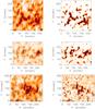 |
Fig. 3 Observed O V emission (left column) and O V emission predicted from MDI magnetograms (right column) using optimum fitted parameters, for active regions 1 (top), 2 (middle) and 3 (bottom) from Table 1. Pixel size is 2′′ × 2′′. Contours correspond to absolute magnetic flux density of 90 Mx cm-2. |
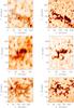 |
Fig. 4 Same as Fig. 3, but for active regions 4 (top), 5 (middle) and 6 (bottom). The black arrow marked “A” in the bottom-left panel shows one of the areas where the observed O V emission is five times brighter than the predicted emission. |
The observed CDS raster is corrected for the effect of the solar rotation which shortens the apparent distance between features in the E-W direction because the CDS slit moves from west to east (direction opposite to the solar rotation) during rastering. Although the effect is small, it may lead to a misalignment of the magnetic and EUV features by up to 6′′ for a 4′ × 4′ raster of 40-min duration. Therefore, the CDS raster is first re-binned to a very fine grid with a step of 0.1′′ along each axis, and then stretched by interpolation along the E-W direction to a spatial grid that is free from the effect of the solar rotation, so that the distance between various features in the E-W direction becomes a true distance on the solar surface. The CDS raster is then re-binned back to a coarser pixel size of 2′′ × 2′′ by averaging twenty 0.1′′ sub-pixels in each direction. This corrected raster is subsequently used for all comparisons with the MDI magnetic field data which also has 2′′ × 2′′ pixels.
To align the MDI and CDS data, a simulated intensity image in the O V 62.97 nm line is calculated from the MDI magnetogram by assuming 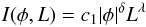 (1)for δ = 0.5, λ = − 0.25 and c1 = 1, where φ is the magnetic flux density in each MDI pixel. This simulated intensity map is smeared out by convolving it with a spatial point spread function (PSF) of the CDS NIS spectrometer. The PSF is a 2D Gaussian with full width at half-maximum FWHMX = 1.7′′ in the E-W direction, FWHMY = 8′′ in the N-S direction (along the slit), and an angle of 12 degrees clockwise from the N-S direction to the longer axis of the Gaussian. The PSF is first calculated with a 0.5′′ step, then each four points along the PSF are summed to provide a representation of PSF with a 2′′ step.
The observed CDS rastered image is then stepped across the large simulated O V image and a cross-correlation function is calculated between the observed CDS image and the simulated CDS image for each relative position of the two arrays. The offset between the two images that gives a maximum value of the cross-correlation is used to align the two arrays, and a sub-array is extracted from the MDI magnetogram with a size equal to the size of the observed O V image. Another sub-array containing corresponding magnetic loop lengths is extracted from the previously calculated loop lengths array.
For further analysis, we assume that the O V line intensity in each pixel is given by Eq. (1). We vary δ from 0 to 1.2 with a step of 0.05. For each value of δ, the index λ is varied from − 0.6 to 0.6 with a step of 0.01. For each pair (δ,λ), a simulated O V intensity is calculated using Eq. (1) with c1 = 1, applied to each pixel of the MDI magnetogram. This 2D array is then convolved with the CDS PSF to give a simulated (predicted) O V image.
To mitigate the effect of a possible misalignment of the CDS and MDI arrays due to a finite, 2′′ × 2′′ pixel size, we subsequently rebin the observed and simulated O V arrays to coarser 4′′ × 4′′ pixels, and use these larger pixels in the fitting process described below.
A preliminary analysis of our data revealed that the relationship given by Eq. (1) does not hold for many of the pixels (see Sect. 3). These pixels are characterised by much higher intensity of the O V line than predicted from Eq. (1), by up to a factor of five. Such outliers can significantly affect the value of χ2 and the resulting fit. We discuss the nature of these deviations in Sect. 3 and conclude that they are caused by short-term temporal variability of the heating episodes and cannot be used to derive the quasi-steady heating.
This finding led us to restrict the range of O V intensities below 3000 erg cm-2 s-1 sr-1 to remove the largest deviations, and fit the model to all points below this threshold, also removing any remaining outliers with unusually low intensities that deviate more than ± 3 standard deviations from the mean value.
For each pair (δ,λ), the constant c1 is calculated to minimise χ2 that compares the observed and simulated intensities for selected pixels:  (2)here, Iobs,i,j and Isim,i,j are local intensities observed and simulated, respectively, in pixel (i,j) and Wi,j are weights. We assume Wi,j = Iobs,i,j.
In addition, we also use a secondary goodness-of-fit criterion, the least absolute deviation, that is less sensitive to occasional outliers in data. It minimises the sum of the absolute value of the residuals:  (3)The least absolute deviation fit adds a constant c0 to Eq. (1).
A second, novel way of fitting the model is to adjust its parameters to reproduce the shape of the lower boundary of the observed O V intensities. This is equivalent to making an assumption that the lower boundary represents the minimum basal heating and any statistically significant deviations from it result from time-variable heating. This approach has been adopted in retrospect, when the first method revealed that the data points show a large scatter around the fitted model.
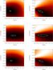 |
Fig. 5 Dependence of χ2 (left column) and S (right column) on the power indeces δ and λ for active region 1 (top), 2 (middle) and 3 (bottom) from Table 1. Contours correspond to 2% and 1% above the minimum values for χ2 and S, respectively. |
3. Results
Table 2 lists the optimum values of (c1,δ,λ) that give the minimum of χ2 (Eq. (2)), and optimum (c0,c1,δ,λ) that give the minimum of S (Eq. (3)). As stated in Sect. 2.1, the model is fitted to all points below the intensity threshold of 3000 erg cm-2 s-1 sr-1 for each active region. These fitted parameters can be different for different regions. The two fitting criteria, χ2 and S, can also give different parameters for a given region. An average value of all values of δ is 0.4, with a standard deviation of 0.1. An average value of all values of λ is − 0.15 with a standard deviation of 0.07. The dependence on L for individual active regions has been determined for the first time from spatially resolved analysis.
Figures 3 and 4 show images of the observed O V intensities and the predicted intensities for the optimum values of δ and λ. Contours show the absolute magnetic flux density | B | = 90 Mx cm-2.
Figures 5 and 6 show how χ2 and S vary with δ and λ for each active region. The plots are colour-coded so that lower values of χ2 and S are darker and high values are white. The crosses show the minimum of χ2 and S. The contours for χ2 is 2% above the minimum value, and the contours for S are 1% above the minimum value.
Figures 7 and 8 (left columns) show the comparison of simulated and observed O V intensities for all six active regions, for the optimum value of (δ,λ). Plots in the right column of Figs. 7 and 8 show the same relationship after the observed O V intensities have been sorted in the same order as ascending simulated intensities, and then smoothed with a 5-point running average. This procedure significantly reduces the scatter and the points are well aligned along the y = x line, suggesting that the scatter is due to a random process.
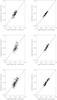 |
Fig. 7 Comparison of observed and simulated O V intensities (I ∝ |φ| δLλ) for the optimum values of δ and λ, for active regions 1 (top), 2 (middle) and 3 (bottom) – see Table 1 for region details. Intensities are in units of erg cm-2 s-1 sr-1. Panels in the left column show the original data, where crosses denote pixels with absolute magnetic flux density φ > 90 Mx cm-2, used to calculate χ2. Pixel size is 4′′ × 4′′. Panels in the right column show the observed O V intensities smoothed with a 5-point running average. The continuous line is an y = x relationship. |
Figures 9 and 10 show the comparison of the simulated and observed intensities in a different way. Here, the simulated intensities I(φ,L) from Eq. (1) (shown previously in the right-hand side of Figs. 3 and 4) have been re-calculated for the optimum fitted value of δ and λ and sorted in ascending order. They are shown as continuous lines. The X axis in these plots is the number index of this sorted, simulated intensity array – the values on the X axis are always integers going from 1,2,3,... to the total number of pixels used in the analysis. Subsequently, the observed intensities have been sorted in the same order as the simulated intensities and overplotted as crosses. This plot allows us to compare the scatter of observed intensities corresponding to each value of the simulated intensity.
The Y axis in Figs. 9 and 10 has been normalised to a common value of 8000 erg cm-2 s-1 sr-1. These plots illustrate that three of the active regions: region 2 (Fig. 9), region 4 and 6 (Fig. 10), contain areas with very high intensities, up to a factor of five greater than the predicted intensities. Moreover, one can see that there is a large scatter of observed intensities in these three regions, significantly exceeding statistical variation, as discussed below. Since the largest scatter is present for stronger magnetic fields, we assume that this scatter is due to time-variable heating that cannot be described by the model given by Eq. (1).
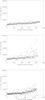 |
Fig. 9 Comparison of observed OV line intensities with the fitted model (I ∝ |φ| δLλ) for optimum δ and λ, for active regions 1 (top), 2 (middle) and 3 (bottom), using 4′′ × 4′′ pixels. Intensities are in units of erg cm-2 s-1 sr-1. The continuous line are fitted values, sorted in ascending order. Crosses are corresponding observed intensities. These plots include all pixels with |B| > 90 Mx cm-2. |
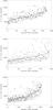 |
Fig. 11 Comparison of observed and predicted OV line intensities for active regions No. 1 (top panel), 2 (middle) and 3 (bottom), using 4′′ × 4′′ pixels. Intensities are in units of erg cm-2 s-1 sr-1. The dashed line is Ilow = Ibou − 3σbou (Eq. (4)), and dash-dotted line is Iup = Ibou + 3σbou, where Ibou is given by Eq. (5). Simulated intensities are sorted in the ascending order. Crosses are corresponding observed intensities sorted in the same order as Ilow. The continuous lines are predicted intensities for optimal fitted δ and λ, sorted in the same order as Ilow. |
Figures 11 and 12 are similar to Figs. 9 and 10, but the Y axis has been limited to 3000 erg cm-2 s-1 sr-1. Another difference is that the simulated intensities are calculated for a common value of δ = 0.45 and λ = − 0.20 for all six regions (see Eq. (5)). As before, these simulated intensities have been sorted in ascending order. The crosses are observed intensities sorted in the same order as the simulated intensities. The optimal fitted model (for optimal δ and λ from Table 2) is shown again as a continuous line. The other two lines shown in these plots, dashed and dash-dotted, will be explained below.
The scatter of points around the fitted model is still significantly greater than ± 3σ, suggesting that possibly most of the areas of the active regions undergo time-variable heating. Our second approach, therefore, is to fit a model to a band of points closest to the lower boundary of the plot in Figs. 11 and 12. This would represent the minimum basal heating level. We have found that the following formula:  (4)matches the lower boundary of the scatter plot in Figs. 11 and 12 for active regions 2–6, where Ibou is given by the empirical equation:
 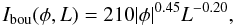 (5)here, φ is expressed in Mx cm-2, L in arcseconds, and intensity in erg cm-2 s-1 sr-1. The statistical error σbou is calculated as before, using the CDS formula from Thompson (1998). For the exposure time of 15 s and using the intensity units as listed above,
  .
.
We find that Ilow given by Eqs. (4) and (5) produces acceptable representation of the shape and the absolute scaling of the lower boundary for five out of the six active regions (shown as dashed line in Figs. 11 and 12). The dash-dotted line in Figs. 11 and 12 represents Iup = Ibou + 3σbou and is therefore greater by 6σbou than the lower boundary Ilow. The range between Ilow and Iup can be explained by statistical variations. This range, however, is quite narrow. As shown in the last column marked P% in Table 2, over 75% of points in regions No. 2–6 have intensities greater than Iup. The average intensity enhancement above Iup for these points is given in the last column marked ER. These deviations must be explained by other processes.
The only region where Ilow does not quite match the lower boundary of the plot is region 1. The dashed line and dash-dotted line for region 1 in Fig. 11 were adjusted by multiplying Ibou by 1.25. Since region 1 is the earliest in time of the six regions, this deviation could indicate that the time-dependent part of the intensity calibration of the CDS/NIS spectrometer may need to be corrected.
The errors of the three parameters in Eq. (5) are estimated in the following way. We used the average fitted δ and λ as a starting point, initially adjusting only C1 to match the lower boundary. We find that δ does not require adjustment, therefore, we use the average error on δ as derived from the fit: δ = 0.45 ± 0.1. Some disagreement between the observations and the model can be seen near the end of the distribution, and can be removed by changing the value of λ. Lambda affects how steep the boundary is near the end of the distribution – the curve becomes steeper with increasing λ. For λ = 0.15 the curve is too flat, for λ = 0.25 the curve is too steep. Therefore, we use λ = 0.20 ± 0.05, where the error 0.05 is close to the error of 0.07 obtained from the average of six regions. The relative error of the constant C1 = 210 ± 27 is estimated by averaging (Iup − Ilow) / (2Ibou) for all data points, for delta = 0.45, lambda = 0.20. This relative error is similar in all six active regions, and its average value is ± 13%.
This second approach then attempts to analyse the basal heating responsible for the lowest values of intensities seen in less than 25% of pixels in regions 2–6. It can be seen from Figs. 11 and 12 that all regions at all values of the magnetic field show significant deviations above this minimum-heating state.
In addition to statistical errors, there are at least four other possible reasons for the deviations of the O V intensity from the model predicted from Eq. (1): (1) in some loops, the actual loop length may differ from the length derived from the potential magnetic field extrapolation; (2) part of the O V emission may arise at loop tops of very short loops, and not at loop footpoints; (3) the heating mechanism depends on an additional factor other than B and L, for example, non-potentiality of the magnetic field; (4) time variability of the O V emission on all time scales, from minutes to tens of minutes, due to the heating mechanism in many loops being highly intermittent. For example, there may be a sudden release of accumulated magnetic stress, as in flares. In such a case, there can be little change in the photospheric magnetic flux density but a substantial change of the O V line intensity. The CDS raster takes 40 min to complete. Moreover, sometimes there is a difference of up to one hour between the time of the magnetogram and the start of the CDS raster. Therefore, it is likely that the line intensities change in this time period. In particular, the OV emission can be quite variable on time scales of the order of minutes to tens of minutes. Figure 13 shows an example of a time series taken in the O V line in an active region plage (NOAA8249 on 23 June 1998). This region was previously analysed for the presence of oscillations in a sunspot plume (Fludra 1999). Here we present a time series in a plage area near a sunspot, recorded in a 4′′ × 3.4′′ pixel. In this two-hour interval the O V intensity shows bursts by up to 100% on time scales of several minutes. This is quite a typical behaviour of the O V intensity in brighter areas of many active region plages. For this time series, the 1σ statistical error is in the range 4–6%, so the variations are real. Another example of variable O V emission in active regions is given by Fludra et al. (1997; see their Fig. 9). Parnell et al. (2002) describe a particular type of transition region brightenings named “active region blinkers” that have intensity enhancement between a factor of 1.8 and 3.3 and lifetime of approximately 16–19 min. These events are attributed to density enhancement; (5) the final possible reason partially responsible for the deviations from the model is the fact that the photospheric magnetic field also evolves and can change both its spatial distribution and the flux density on time scales of one hour, separating the CDS rasters and MDI magnetograms, thus also contributing to the scatter.
3.1. Coronal heating
Clearly, on small spatial scales (4′′ × 4′′ pixels) the relationship between the O V 62.97 nm line intensity and the magnetic flux density has much greater scatter than in spatially integrated IT − Φ plots (see Fludra & Ireland 2008; their Fig. 4). We attribute this scatter largely to a time variable heating component. We defer addressing the mechanism of the time variable heating to a future paper. Here we consider the hypothesis that the lower boundary of the scatter plots in Figs. 11 and 12, which we called the basal heating, represents a quasi-steady heating component and we use the assumption of static loops to infer the heating rate for this component.
The intensity of a transition region line emitted from a static loop is (Martens et al. 2000; Fludra & Ireland 2008, their Eq. (7)): 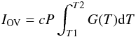 (6)where P is plasma pressure and G(T) is the line emissivity. Combining this with Eq. (5), we obtain P ∝ φ0.45 L-0.20. For static loops, where
  (Rosner et al. 1978), we obtain the volumetric heating rate Eh ∝ φ0.5L-1.
The power index of 0.5 is lower than the range of 0.6 − 1.1 derived from the global analysis of the O V emission by Fludra & Ireland (2008). It is also lower than the index of 1.0 obtained by Schrijver & Aschwanden (2002) from simulations of solar and stellar soft X-ray emission, and the index of 0.9 obtained by Yashiro & Shibata (2001) based on data from the Yohkoh Soft X-ray Telescope.
The difference between the result of this paper and the global analysis of Fludra & Ireland (2008) of the same O V spectral line can be explained by the fact that the global analysis does not separate the time variable and quasi-static heating. Intensities of all pixels are summed, and all high-intensity pixels therefore contribute to the total intensity. These pixels, with the largest intensity scatter present in high-B pixels, could make the slope of the I − B relationship steeper in the global analysis. This is an additional factor to be added to the warnings stated by Fludra & Ireland (2008) that the global analysis is a rather inadequate tool for diagnosing the coronal heating mechanism.
A comparison with results obtained for the coronal emission is more difficult. First, the same explanation applies as in the previous paragraph, as all coronal results are also based on spatially-integrated quantities. Intensities produced by time-variable heating are then summed and analysed together with those arising from the quasi-steady heating. However, the coronal emission in active region loops does not appear to fluctuate as rapidly and with as high amplitude as the transition region emission, with the exception of flaring episodes. The question therefore remains as to whether we are comparing the same heating process – it is possible that the basal heating observed in the O V transition region line in the pixels comprising the lower boundary in Figs. 11 and 12, and the heating of loop tops observed in coronal lines are two independent processes taking place at different heights or occurring in magnetic structures not connected with each other. However, even if this basal O V emission was due to unresolved events on small spatial scales originating in magnetic threads that are far from equilibrium, the existence of a common lower boundary in five active regions suggests that this emission is generated by a universal process well predictable from the magnetic flux density.
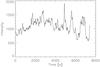 |
Fig. 13 2-h time series of the intensity of the O V 62.97 nm line from a 4′′ × 3.4′′ pixel, in an active region plage of NOAA 8249 on 23 June 1998. The intensity has been multiplied by the exposure time of 10 s and is expressed in photons. |
4. Summary
In this paper we have expanded the previous analyses of the relationships between the EUV and X-ray intensities, and the magnetic flux. Fludra & Ireland (2008) discussed the inadequacy of the global, spatially integrated quantities for the determination of the coronal heating mechanism. We have therefore used spatially resolved data to study these relationships on a pixel-by-pixel basis. We have analysed six active regions, observed by the SOHO CDS in the transition region line O V 62.97 nm. The CDS rastered images were co-aligned with the magnetic flux density extracted from full disk SOHO MDI magnetograms, and the O V line intensities in each CDS pixel were compared with the magnetic flux density. We have found that in three of the active regions (region 2, 4 and 6 from Table 1) there are areas of highly enhanced O V intensities that deviate from the relationship given by Eq. (1) by up to a factor of five. These enhanced intensities are associated with stronger magnetic field concentrations and are attributed to micro-flaring events. These pixels have been omitted from the fitting of Eq. (1). When the intensities below the threshold of 3000 erg cm-2 s-1 sr-1 were fitted with Eq. (1), the derived power indeces, averaged over the six active regions, are δ = 0.4 ± 0.1, λ = − 0.15 ± 0.07. The scatter around this fit is still significantly greater than ± 3σ statistical error. This can be caused by a number of effects: imprecise alignment of the MDI and CDS arrays due to a finite pixel size, temporal variability of O V intensities, non-potential nature of the magnetic field affecting the estimates of the loop lengths, or the need for a more complex heating model, involving other quantities in addition to φ and L.
We have subsequently adjusted the parameters of the model to match the lower boundary of the O V intensity distribution in Figs. 11 and 12, and obtained δ = 0.45, λ = − 0.20, c1 = 210 (Eq. (5)). We suggest that this represents a basal heating of the transition region plasma in active regions through a universal process that is well characterised by the magnetic loop density and loop length.
In summary:
-
(1)
We have shown that the relationship between theO V intensities and the magnetic field on smallspatial scales of a few arcseconds is characterised by a largescatter much greater than the statistical noise and greater than thatseen for the global, spatially-integrated quantities.
-
(2)
We have found for the first time an empirical formula that provides a lower boundary on the O V intensities that can be predicted from the magnetic flux density and loop length. The existence of this lower boundary, common to five of the analysed active regions, demonstrates conclusively the primary role of the magnetic field in heating the transition region plasma.
-
(3)
The scatter of intensities above the lower boundary, over and above the statistical noise, is highly suggestive of the presence of ubiquitous temporal variability of the intensities. The energy input to the magnetic loops in active regions is therefore likely to be variable in time, and the formula linking the heating rate to the magnetic field should include time-variable effects in addition to the photospheric magnetic flux density (or field strength) and loop length.
-
(4)
We have therefore demonstrated that: (a) the spatially-resolved analysis shows the presence of the basal heating in less than 25% of pixels. If this basal relationship between the intensities of the O V line and the magnetic flux density is attributed to steady heating, we can estimate the dependence of the volumetric heating rate on φ and L using scaling laws for static loops; (b) this analysis can detect deviations from the basal heating and identify areas of strongly enhanced intensities which undergo micro-flaring.
This is the first detailed analysis of the relationship between the EUV transition region emission and the magnetic field in active regions, done using spatially resolved EUV line intensities and photospheric magnetograms. This work reveals a great complexity of the problem, where the basal heating can be masked by a significant temporal variability of the transition region emission in active region loops. Past analyses using spatially-integrated quantities were unable to distinguish between the steady and variable components. It is clear that observations with high temporal and spatial resolution, and a good alignment between the EUV emission and vector magnetic data are necessary to solve the coronal heating problem.
Acknowledgments
This work was supported by the UK Science and Technology Facilities Council. SOHO is a project of international cooperation between ESA and NASA. CDS was built and is operated by a consortium led by the Rutherford Appleton Laboratory and including the Mullard Space Science Laboratory, the NASA Goddard Space Flight Center, Oslo University and the Max-Planck-Institute for Extraterrestrial Physics, Garching. The authors thank Dr T. Hoeksema for information on the performance of the SOHO MDI instrument.
References
- Aschwanden, M. J., Newmark, J. S., Delaboudiniere, J.-P., et al. 1999, ApJ, 515, 842 [NASA ADS] [CrossRef] [Google Scholar]
- Fisher, G. H., Longcope, D. W., Metcalf, T. R., & Pevtsov, A. A. 1998, ApJ, 508, 885 [NASA ADS] [CrossRef] [Google Scholar]
- Fludra, A. 1999, A&A, 344, L75 [NASA ADS] [Google Scholar]
- Fludra, A., & Ireland, J. 2003, A&A, 398, 297 [NASA ADS] [CrossRef] [EDP Sciences] [Google Scholar]
- Fludra, A., & Ireland, J. 2004, in Stars as Suns – Activity, Evolution, and Planets, ed. A. K. Dupree, & A. O. Benz, IAU Symp., ASP Conf. Ser., 219, 478 [Google Scholar]
- Fludra, A., & Ireland, J. 2008, A&A, 483, 609 [NASA ADS] [CrossRef] [EDP Sciences] [Google Scholar]
- Fludra, A., Brekke, P., Harrison, R. A., et al. 1997, Sol. Phys., 175, 487 [NASA ADS] [CrossRef] [Google Scholar]
- Fludra, A., Ireland, J., Del Zanna, G., & Thompson, W. T. 2002, Adv. Space Res., 29, 3, 361 [NASA ADS] [CrossRef] [Google Scholar]
- Harrison, R. A., Sawyer, E. C., Carter, M. K., et al. 1995, Sol. Phys. 162, 233 [Google Scholar]
- Harrison, R. A., Lang, J., Brooks, D. H., & Innes, D. E. 1999, A&A, 351, 1115 [NASA ADS] [Google Scholar]
- Jordan, C., Smith, G. R., & Houdebine, E. R. 2005, MNRAS, 362, 411 [NASA ADS] [CrossRef] [Google Scholar]
- Martens, P. C. H., Kankelborg, C. C., & Berger, T. E. 2000, ApJ, 537, 471 [NASA ADS] [CrossRef] [Google Scholar]
- Parnell, C. E., Bewsher, D., & Harrison, R. A. 2002, Sol. Phys., 206, 249 [NASA ADS] [CrossRef] [Google Scholar]
- Pevtsov, A. A., Fisher, G. H., Acton, L. W., et al. 2003, ApJ, 598, 1387 [NASA ADS] [CrossRef] [Google Scholar]
- Rosner, R., Tucker, W. H., & Vaiana, G. S. 1978, ApJ, 220, 643 [NASA ADS] [CrossRef] [Google Scholar]
- Scherrer, P. H., Bogart, R. S., Bush, R. I., et al. 1995, Sol. Phys., 162, 129 [Google Scholar]
- Schrijver, C. J., & Aschwanden, M. J. 2002, ApJ, 566, 1147 [NASA ADS] [CrossRef] [Google Scholar]
- Tarbell, T., Ryutova, M., Covington, J., & Fludra, A. 1999, ApJ, 514, L47 [NASA ADS] [CrossRef] [Google Scholar]
- Thompson, W. T. 1998, CDS Software Note 49 [Google Scholar]
- Warren, H. P., & Winebarger, A. R. 2006, ApJ, 645, 711 [NASA ADS] [CrossRef] [Google Scholar]
- Yashiro, S., & Shibata, K. 2001, ApJ, 550, L113 [NASA ADS] [CrossRef] [Google Scholar]
All Tables
All Figures
|
Fig. 1 MDI magnetograms for active regions 1 (top), 2 (middle) and 3 (bottom) from Table 1. Contours correspond to absolute magnetic flux density of 90 Mx cm-2. Bmax,b and Bmax,w are maximum values (Mx cm-2) of the negative (black) and positive (white) polarity, respectively. |
| In the text | |
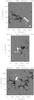 |
Fig. 2 Same as Fig. 1, but for active regions 4 (top), 5 (middle) and 6 (bottom). |
| In the text | |
|
Fig. 3 Observed O V emission (left column) and O V emission predicted from MDI magnetograms (right column) using optimum fitted parameters, for active regions 1 (top), 2 (middle) and 3 (bottom) from Table 1. Pixel size is 2′′ × 2′′. Contours correspond to absolute magnetic flux density of 90 Mx cm-2. |
| In the text | |
|
Fig. 4 Same as Fig. 3, but for active regions 4 (top), 5 (middle) and 6 (bottom). The black arrow marked “A” in the bottom-left panel shows one of the areas where the observed O V emission is five times brighter than the predicted emission. |
| In the text | |
|
Fig. 5 Dependence of χ2 (left column) and S (right column) on the power indeces δ and λ for active region 1 (top), 2 (middle) and 3 (bottom) from Table 1. Contours correspond to 2% and 1% above the minimum values for χ2 and S, respectively. |
| In the text | |
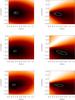 |
Fig. 6 Same as Fig. 5, but for active region 4 (top), 5 (middle) and 6 (bottom). |
| In the text | |
|
Fig. 7 Comparison of observed and simulated O V intensities (I ∝ |φ| δLλ) for the optimum values of δ and λ, for active regions 1 (top), 2 (middle) and 3 (bottom) – see Table 1 for region details. Intensities are in units of erg cm-2 s-1 sr-1. Panels in the left column show the original data, where crosses denote pixels with absolute magnetic flux density φ > 90 Mx cm-2, used to calculate χ2. Pixel size is 4′′ × 4′′. Panels in the right column show the observed O V intensities smoothed with a 5-point running average. The continuous line is an y = x relationship. |
| In the text | |
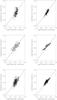 |
Fig. 8 Same as Fig. 7, but for active regions 4 (top), 5 (middle) and 6 (bottom). |
| In the text | |
|
Fig. 9 Comparison of observed OV line intensities with the fitted model (I ∝ |φ| δLλ) for optimum δ and λ, for active regions 1 (top), 2 (middle) and 3 (bottom), using 4′′ × 4′′ pixels. Intensities are in units of erg cm-2 s-1 sr-1. The continuous line are fitted values, sorted in ascending order. Crosses are corresponding observed intensities. These plots include all pixels with |B| > 90 Mx cm-2. |
| In the text | |
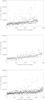 |
Fig. 10 Same as Fig. 9, but for active regions 4 (top), 5 (middle) and 6 (bottom). |
| In the text | |
|
Fig. 11 Comparison of observed and predicted OV line intensities for active regions No. 1 (top panel), 2 (middle) and 3 (bottom), using 4′′ × 4′′ pixels. Intensities are in units of erg cm-2 s-1 sr-1. The dashed line is Ilow = Ibou − 3σbou (Eq. (4)), and dash-dotted line is Iup = Ibou + 3σbou, where Ibou is given by Eq. (5). Simulated intensities are sorted in the ascending order. Crosses are corresponding observed intensities sorted in the same order as Ilow. The continuous lines are predicted intensities for optimal fitted δ and λ, sorted in the same order as Ilow. |
| In the text | |
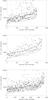 |
Fig. 12 Same as Fig. 11, but for active regions 4 (top panel), 5 (middle) and 6 (bottom). |
| In the text | |
|
Fig. 13 2-h time series of the intensity of the O V 62.97 nm line from a 4′′ × 3.4′′ pixel, in an active region plage of NOAA 8249 on 23 June 1998. The intensity has been multiplied by the exposure time of 10 s and is expressed in photons. |
| In the text | |
Current usage metrics show cumulative count of Article Views (full-text article views including HTML views, PDF and ePub downloads, according to the available data) and Abstracts Views on Vision4Press platform.
Data correspond to usage on the plateform after 2015. The current usage metrics is available 48-96 hours after online publication and is updated daily on week days.
Initial download of the metrics may take a while.