| Issue |
A&A
Volume 522, November 2010
|
|
|---|---|---|
| Article Number | L2 | |
| Number of page(s) | 4 | |
| Section | Letters | |
| DOI | https://doi.org/10.1051/0004-6361/201015706 | |
| Published online | 26 October 2010 | |
Letter to the Editor
Turbulent eddy-time-correlation in the solar convective zone
1
Institut d’Astrophysique et de Géophysique, Université de
Liège,
Allée du 6 août 17,
4000
Liège,
Belgium
2
LESIA, UMR8109, Université Pierre et Marie Curie, Université Denis
Diderot, Obs. de Paris, 92195
Meudon Cedex,
France
e-mail: This email address is being protected from spambots. You need JavaScript enabled to view it.
3
Institut d’Astrophysique Spatiale, CNRS-Université Paris XI UMR
8617, 91405
Orsay Cedex,
France
4
Instituto de Astrofísica de Canarias, 38200 La Laguna, Tenerife, Spain
5
Departamento de Astrofísica, Universidad de La
Laguna, 38206 La
Laguna, Tenerife,
Spain
Received:
7
September
2010
Accepted:
6
October
2010
Abstract
Theoretical modeling of the driving processes of solar-like oscillations is a powerful way of understanding the properties of the convective zones of solar-type stars. In this framework, the description of the temporal correlation between turbulent eddies is an essential ingredient to model mode amplitudes. However, there is a debate between a Gaussian or Lorentzian description of the eddy-time correlation function (Samadi et al. 2003b, A&A, 403, 303; Chaplin et al. 2005, MNRAS, 360, 859). Indeed, a Gaussian description reproduces the low-frequency shape of the mode amplitude for the Sun, but is unsatisfactory from a theoretical point of view (Houdek 2010, Ap&SS, 328, 237) and leads to other disagreements with observations (Samadi et al. 2007, A&A, 463, 297). These are solved by using a Lorentzian description, but there the low-frequency shape of the solar observations is not correctly reproduced. We reconcile the two descriptions by adopting the sweeping approximation, which consists in assuming that the eddy-time-correlation function is dominated by the advection of eddies, in the inertial range, by energy-bearing eddies. Using a Lorentzian function together with a cut-off frequency derived from the sweeping assumption allows us to reproduce the low-frequency shape of the observations. This result also constitutes a validation of the sweeping assumption for highly turbulent flows as in the solar case.
Key words: convection / turbulence / Sun: oscillations
© ESO, 2010
1. Introduction
Excitation of solar-like oscillations is attributed to turbulent motions that excite p modes (for a recent review, see Samadi 2009). Their amplitudes result from a balance between excitation and damping and crucially depend on the way the eddies are temporally correlated as shown for solar p and g modes (Samadi et al. 2003b; Belkacem et al. 2009b; Appourchaux et al. 2010), for main-sequence stars (Samadi et al. 2010b,a), for red giants (Dupret et al. 2009), or for massive stars (Belkacem et al. 2009a, 2010). Hence, the improvement of our understanding and modeling of the temporal correlation of turbulent eddies, hereafter denoted in the Fourier domain as χk(ω), is fundamental to infer turbulent properties in stellar convection zones.
There are two ways to compute the eddy-time correlation function. A direct computation from 3D numerical simulations is possible and was performed by Samadi et al. (2008a). Nevertheless, Samadi (2009) pointed out that the results depend on the spatial resolution, and therefore dedicated high-resolution 3D numerical simulations are required. This then becomes an important limitation when computing mode amplitudes for a large number of stars, preventing us from applying statistical astereosismology.
The second way to compute χk consists in using appropriate analytical descriptions. Most of the theoretical formulations of mode excitation explicitly or implicitly assume a Gaussian functional form for χk(ω) (Goldreich & Keeley 1977; Dolginov & Muslimov 1984; Goldreich et al. 1994; Balmforth 1992; Samadi et al. 2001; Chaplin et al. 2005). However, 3D hydrodynamical simulations of the outer layers of the Sun show that at the length-scales close to those of the energy-bearing eddies (around 1 Mm), χk is a Lorentzian function (Samadi et al. 2003a; Belkacem et al. 2009b). As pointed out by Chaplin et al. (2005), a Lorentzian χk is also a result predicted for the largest, most-energetic eddies by the time-dependent mixing-length formulation derived by Gough (1977). Therefore, there is numerical, theoretical, and also observational evidence (Samadi et al. 2007) that χk is Lorentzian.
However, Chaplin et al. (2005), Samadi (2009), and Houdek (2010) found that a Lorentzian χk, when used with a mixing-length description of the whole convection zone, results in a severe over-estimate for the low-frequency modes. In this case, low-frequency modes (ν < 2 mHz) are excited deep in the solar convective region by large-scale eddies that give a substantial fraction of the energy injected to the modes. Chaplin et al. (2005) and Samadi (2009) then suggested that most contributing eddies situated deep in the Sun have a χk more Gaussian than Lorentzian because at a fixed frequency, a Gaussian χk decreases more rapidly with depth.
We therefore propose a refined description of the eddy-time correlation function based on the sweeping approximation to overcome this issue. This consists in assuming that the temporal correlation of the eddies, in the inertial subrange, is dominated by the advection by energy-bearing eddies. This assumption was first proposed by Tennekes (1975), and was subsequently investigated by Kaneda (1993) and Kaneda et al. (1999). In this letter, we demonstrate that the low-frequency shape of the observed energy injection rates into the solar modes is very sensitive to this assumption and more precisely to the Eulerian microscale, defined as the curvature of the time-correlation function at the origin. Hence, modeling of the solar p-mode amplitudes is shown to constitute an efficient test for temporal properties in highly turbulent flows.
The paper is organized as follows: Sect. 2 defines the eddy-time correlation function. In Sect. 3, we propose a short-time expansion of the eddy-time correlation function. The use of the Eulerian microscale as a cut-off is introduced in the computation of solar p mode amplitudes and the result is compared to the observations in Sect. 4. Finally, Sect. 5 is dedicated to conclusions and discussions.
2. The Eulerian eddy time-correlation function
For a turbulent fluid, one defines the Eulerian eddy time-correlation function as
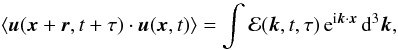 (1)
(1)
where u is the Eulerian turbulent velocity field, x and t the space and time position of the fluid element, k the wave number vector, τ the time-correlation length, and r the space-correlation length. The function ℰ in the RHS of Eq. (1) represents the time-correlation function associated with an eddy of wave-number k.
We assume an isotropic and stationary turbulence, accordingly ℰ is only a function of k and τ. The quantity ℰ(k,τ) is related to the turbulent energy spectrum according to
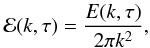 (2)
(2)
where E(k,τ) is the turbulent kinetic energy spectrum whose temporal Fourier transform is
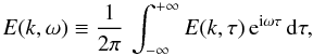 (3)
(3)
where ω is the eddy frequency, and E(k,ω) is written following an approximated form proposed by Stein (1967)
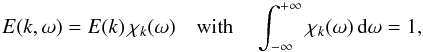 (4)
(4)
where χk(ω) is the frequency component of E(k,ω). In other words, χk(ω) represents – in the frequency domain – the temporal correlation between eddies of wave-number k.
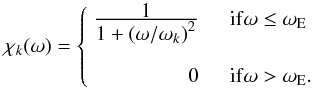
As already discussed in Sect. 1, theoretical and observational evidence show that χk(ω) is Lorentzian, i.e.
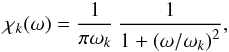 (5)
(5)
where ωk is by definition the width at half maximum of χk(ω). In the framework of Samadi & Goupil (2001)’s formalism, this latter quantity is evaluated as:
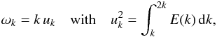 (6)
(6)
where E(k) is defined by Eq. (4). However, in the high-frequency regime (ω ≫ ωk), corresponding to the short-time correlation (τ ≈ 0), the situation is less clear. We next investigate short-time correlations (τ ≈ 0).
3. The sweeping assumption for the Eulerian time-correlation function
3.1. Short-time expansion of the eddy-time correlation function
The function ℰ(k,t,τ) (Eq. (1)) can be expanded for short-time scales, in the inertial sub-range (i.e. for k > k0 and k < kd, where k0 is the wave number of energy-bearing eddies and kd is the wave-number of viscous dissipation), using the Navier-Stokes equations and the sweeping assumption, as (see Kaneda 1993, for a derivation)
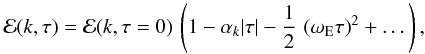 (7)
(7)
where the characteristic frequency αk is defined by the relation
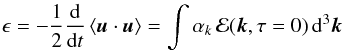 (8)
(8)
with ϵ the dissipation rate of energy. Hence, αk is the typical frequency of energy dissipation at the scale k. It can be estimated by assuming that a large fraction of the kinetic energy of eddies is lost within one turnover time (Tennekes & Lumley 1972). Hence, αk is approximated by the turn-over frequency αk = kuk = ωk (see Eq. (6)).
The second characteristic frequency, ωE(k), is the curvature of the correlation function near the origin (Kaneda 1993), and is defined by
 (9)
(9)
The associated
characteristic time  is also
referred to as the Eulerian micro-scale1 (Tennekes & Lumley 1972). An approximate
expression for ωE(k) can be obtained by
assuming the random sweeping effect of large eddies on small eddies. This assumption
consists in assuming that the velocity field
u(k) associated with an eddy of
wave-number k lying in the inertial-subrange (i.e. large
k compared to
k0) is advected by the energy-bearing eddies
with velocity u0 (i.e. of wave-number
k0). This time-scale is obtained by assuming
uniform density, which is valid in the Sun for
k > k0
(i.e. in the inertial sub-range) since the density scale-height approximately equals the
length-scale of energy-bearing eddies
((dlnρ / dr)-1 ≈ 2π / k0).
It also assumes the quasi-normal approximation (see Kaneda
1993; Kaneda et al. 1999; Rubinstein & Zhou 2002, for details). The
Eulerian micro-scale then corresponds to the timescale over which the energy-bearing
eddies of velocity u0 advect eddies of size
2πk-1. It is the lowest time-scale (highest
frequency) on which those eddies can be advected.
is also
referred to as the Eulerian micro-scale1 (Tennekes & Lumley 1972). An approximate
expression for ωE(k) can be obtained by
assuming the random sweeping effect of large eddies on small eddies. This assumption
consists in assuming that the velocity field
u(k) associated with an eddy of
wave-number k lying in the inertial-subrange (i.e. large
k compared to
k0) is advected by the energy-bearing eddies
with velocity u0 (i.e. of wave-number
k0). This time-scale is obtained by assuming
uniform density, which is valid in the Sun for
k > k0
(i.e. in the inertial sub-range) since the density scale-height approximately equals the
length-scale of energy-bearing eddies
((dlnρ / dr)-1 ≈ 2π / k0).
It also assumes the quasi-normal approximation (see Kaneda
1993; Kaneda et al. 1999; Rubinstein & Zhou 2002, for details). The
Eulerian micro-scale then corresponds to the timescale over which the energy-bearing
eddies of velocity u0 advect eddies of size
2πk-1. It is the lowest time-scale (highest
frequency) on which those eddies can be advected.
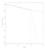 |
Fig. 1 Schematic time-correlation (χk) versus normalized eddy frequency (ω / ωE) at k = 5k0 (i.e. in the inertial subrange such as kd ≫ k > k0), where k0 = 6.28 × 10⁻⁶ m-1. Note that the value of k0 does not influence the result. The solid line (resp. dashed triple dot line) correponds to the Lorentizan functional form of χk for ω < ωE (resp. ω < ωE). The dashed line corresponds to a Gaussian modeling (χk ∝ e − (ω / ωE)2) of characteristic frequency ωE. (we numerically verified that e − (τ / τE)2 is a good approximation of Eq. (7), see also Sect. 3.2). We stress that the sharp decrease the functional form given by Eq. (7), in the temporal Fourier domain, then justifies to consider ωE as a cut-off frequency. In other words, χk is computed according to Eq. (12). |
3.2. Eulerian time micro-scale as a cut-off frequency
The issue is now to estimate to what extent ωE can be considered as a cut-off frequency, i.e. that there is a sharp change in the slope of χk at high ω.
To this end, we first remark that the zero-th- and first-order terms in Eq. (7) are consistent with an exponential decrease of width αk (i.e. a Lorentzian in the frequency domain of width ωk, Eq. (5)) for small τ. In contrast, the zero-th-order term together with the second order term in Eq. (7) are consistent with a Gaussian behavior of width τE. Hence, the relative importance of those two regimes depends on the relative magnitude of the second and third terms in Eq. (7). Let us define the ratio (ℛ) of the first to the second order term in the expansion of ℰ (Eq. (7))
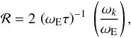 (10)
(10)
To evaluate this ratio,
we compare the typical frequencies ωk and
ωE using Eq. (9) together with Eq. (6).
Adopting a Kolmogorov spectrum
E(k) = CKϵ2 / 3k − 5 / 3,
with CK the Kolmogorov universal constant
(close to 1.72), we have 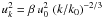 , where
β = 0.555. Hence
, where
β = 0.555. Hence
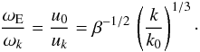 (11)
(11)
From Eq. (11) we conclude that for k ≫ k0 (i.e. at small scale) we have ωE / ωk ≈ β − 1 / 2(k / k0)1 / 3 ≫ 1, then τE ≪ τk. And for k ≈ k0 (i.e. at large scale), we have ωE / ωk = β − 1 / 2 ≈ 1.4. Hence, we always are in the situation where ωE > ωk.
From Eq. (10), it immediately follows that for ω ≳ ωE the second order term dominates over the first order one in Eq. (7), at all length-scales. We then conclude that for frequencies near the micro-scale frequency (ω ≳ ωE), the eddy-time correlation function behaves as a Gaussian function (e − (ω / ωE)2) instead of a Lorentzian function, resulting in a sharp decrease with ω (see Fig. 1). Hence, the contributions for ω > ωE are negligible and the temporal correlation is computed as follows
 (12)
(12)
4. Computation of the p-mode energy injection rates
4.1. Computation of the energy injection rate
The formalism we used to compute excitation rates of radial modes was developed by Samadi & Goupil (2001) and Samadi et al. (2005) (see Samadi 2009, for a thorough discussion)
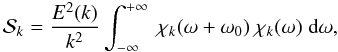
For a radial mode of frequency ω0 = 2πν0, the excitation rate (or equivalently, the energy injection rate), P, mostly arises from the Reynolds stresses and can be written as (see Eq. (21) of Belkacem et al. 2008)
![Mathematical equation: \begin{eqnarray} \label{puissance} P(\omega_0) = \frac{\pi^{3}}{2 I} \int_{0}^{M} \, \left[ \rho_0 \, \left(\frac{16}{15}\right) \left(\frac{\partial \xi_r}{\partial r}\right)^2 \; \int_{0}^{+\infty} \mathcal{S}_k \; \textrm{d}k \right] \textrm{d}m \label{source} \end{eqnarray}](/articles/aa/full_html/2010/14/aa15706-10/aa15706-10-eq81.png) (13)
(13)
 (14)
(14)
where ξr is the radial component of the fluid displacement eigenfunction (ξ), m is the local mass, ρ0 the mean density, ω0 the mode angular frequency, I the mode inertia, Sk the source function, E(k) the spatial kinetic energy spectrum, χk the eddy-time correlation function, and k the wave-number.
The rate (P) at which energy is injected into a mode is computed according to Eq. (13). In this letter, we consider two theoretical models, namely:
-
–
an analytical approach: the 1D calibrated solar structure modelused for these computations is obtained with the stellar evolutioncode CESAM2k (Morel 1997; Morel & Lebreton 2008). The atmosphere is computedassuming an Eddington grey atmosphere. Convection isincluded according to a Böhm-Vitense mixing-length (MLT)formalism (see Samadiet al. 2006, for details), from whichthe convective velocity is computed. The mixing-lengthparameter α is adjusted in a way that the model reproduces the solar radius and the solar luminosity at the solar age. This calibration gives α = 1.90, with an helium mass fraction of 0.245, and a chemical composition following Grevesse & Noels (1993). The equilibrium model also includes turbulent pressure;
-
–
a semi-analytical approach: calculation of the mode excitation rates is performed essentially in the manner of Samadi et al. (2008a,b). All required quantities, except the eddy-time correlation function, the mode eigenfunctions (ξr) and mode inertia (I), are directly obtained from a 3D simulation of the outer layers of the Sun (see Samadi 2009, for details on the numerical simulation).
In both cases, the eigenfrequencies and eigenfunctions are computed with the adiabatic pulsation code ADIPLS (Christensen-Dalsgaard 2008). We stress again that in both cases χk is implemented as an analytical function.
4.2. Results on mode amplitudes
When the frequency range of χk is extended toward infinity, computation of P according to Eq. (13) and Eq. (14) fails to reproduce the observations, in particular the low-frequency shape. In order to illustrate this issue, we have computed the solar model excitation rates, using the solar global model described in Sect. 4.1. The turbulent kinetic energy spectrum (E(k)) is assumed to be a Kolmogorov spectrum to be consistent with the derivation of τE as proposed by Kaneda (1993). In addition, the eddy-time correlation function is supposed to be Lorentzian as described by Eq. (5) for all ω > 0. In agreement with the results of Chaplin et al. (2005) and Samadi (2009), it results in an over-estimate of the excitation rates at low frequency (see Fig. 2 top).
In contrast, by assuming that the time-dynamic of eddies in the Eulerian point of view is
dominated by the sweeping, the Eulerian time micro-scale arises as a cut-off frequency
(see Sect. 3.2). Hence,
χk(ω) is modeled
following Eq. (5) for
ω < ωE and
χk(ω) = 0 elsewhere. Using
this procedure to model
χk(ω) (i.e. by introducing
ωE as a cut-off frequency) permits us to reproduce the
low-frequency (ν < 3 mHz) shape of the mode
excitation rates as observed by the GONG network (see Fig. 2). This is explained as follows: for large-scale eddies near
 , situated
deep in the convective region, the cut-off frequency ωE is
close to ωk as shown by Eq. (11). As a consequence, the frequency range
over which χk is integrated in Eq. (14) is limited, resulting in lower injection
rates into the modes.
, situated
deep in the convective region, the cut-off frequency ωE is
close to ωk as shown by Eq. (11). As a consequence, the frequency range
over which χk is integrated in Eq. (14) is limited, resulting in lower injection
rates into the modes.
Note that the absolute values of mode excitation rates are not reproduced by using a mixing-length description of convection, this is in agreement with Samadi (2009), and arises because that it underestimates the convective velocities as well as convective length-scales. It then explains the differences between the computation of mode excitation rates using the MLT and the 3D numerical simulations (Fig. 2).
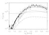 |
Fig. 2 Solar p-mode excitation rates as a function of the frequency ν. The dots correspond to the observational data obtained by the GONG network, as derived by Baudin et al. (2005), and the triangles corresponds to observational data obtained by the GONG network as derived by Salabert et al. (2009) for ℓ = 0 to ℓ = 35. The dashed line corresponds to the computation of the excitation rates using the analytical approach together with a Lorentzien description of χkwithout any cut-off frequency. Note that this modeling is similar to that mentioned by Chaplin et al. (2005). The solid line corresponds to the computation of mode excitation rates using the semi-analytical approach as described in Sect. 4.1 and using a Lorentzian χk together with a cut-off frequency at ω = ωE. The dashed triple dot line corresponds to the analytical approach using a Lorentzian description of χk down to the cut-off frequency ωE. Finally, the dashed-dot line corresponds to a semi-analytical approach using a Gaussian description of χk. Note that both solid (Lorentzian χk) and dashed-dot (Gaussian χk) lines present a similar frequency dependance, and since both are computed using the 3D numerical simulations for the convective motions the differences only comes from the way turbulence is temporally correlated. |
5. Conclusion and discussion
By using a short-time analysis and the sweeping assumption, we have shown that there is a frequency (ωE the micro-scale frequency) beyond the temporal correlation χk sharply decreases with frequency. Including this frequency as a cut-off in our modeling of χk and assuming a Lorentzian shape we are able to reproduce the observed low-frequency (ν < 3 mHz) excitation rates.
These results then re-conciliate the theoretical and observational evidence that the frequency dependence of the eddy-time correlation may be Lorentzian in the whole solar convective region down to the cut-off frequency ωE. Finally, it also represents a validation of the sweeping assumption in highly turbulent flows.
We note, however, that one must remove several theoretical shortcomings to go further. For instance, a rigourous treatment of the energy-bearing eddies is needed. The short-time analysis and the computation of the Eulerian miscro-scale must be reconsidered by including the effect of buoyancy that mainly affects large scales. Furthermore, some discrepancies remain at high-frequency (ν > 3 mHz), and to go beyond these one has to remove the separation of scales assumption (see Belkacem et al. 2008, for a dedicated discussion) and include non-adiabatic effects.
Eventually, we note that the modeling of amplitudes under the sweeping assumption is to be extended. In particular, the investigation of the effect of the sweeping assumption on solar gravity mode amplitudes is desirable.
It is the time equivalent of the Taylor micro-scale, which corresponds to the largest scale at which viscosity affects the dynamic of eddies.
Acknowledgments
We are indebted to J. Leibacher for his careful reading of the manuscript and his helpful remarks. K.B. acknowledges financial support through a postdoctoral fellowship from the Subside fédéral pour la recherche 2010, University of Liège. The authors also acknowledge financial support from the French National Research Agency (ANR) for the SIROCO (SeIsmology, ROtation and COnvection with the COROT satellite) project.
References
- Appourchaux, T., Belkacem, K., Broomhall, A., et al. 2010, A&AR, 18, 197 [CrossRef] [Google Scholar]
- Balmforth, N. J. 1992, MNRAS, 255, 639 [NASA ADS] [Google Scholar]
- Baudin, F., Samadi, R., Goupil, M.-J., et al. 2005, A&A, 433, 349 [NASA ADS] [CrossRef] [EDP Sciences] [Google Scholar]
- Belkacem, K., Samadi, R., Goupil, M.-J., & Dupret, M.-A. 2008, A&A, 478, 163 [NASA ADS] [CrossRef] [EDP Sciences] [Google Scholar]
- Belkacem, K., Samadi, R., Goupil, M., et al. 2009a, Science, 324, 1540 [NASA ADS] [CrossRef] [Google Scholar]
- Belkacem, K., Samadi, R., Goupil, M. J., et al. 2009b, A&A, 494, 191 [NASA ADS] [CrossRef] [EDP Sciences] [Google Scholar]
- Belkacem, K., Dupret, M. A., & Noels, A. 2010, A&A, 510, A6 [NASA ADS] [CrossRef] [EDP Sciences] [Google Scholar]
- Chaplin, W. J., Houdek, G., Elsworth, Y., et al. 2005, MNRAS, 360, 859 [NASA ADS] [CrossRef] [Google Scholar]
- Christensen-Dalsgaard, J. 2008, Ap&SS, 316, 113 [NASA ADS] [CrossRef] [Google Scholar]
- Dolginov, A. Z., & Muslimov, A. G. 1984, Ap&SS, 98, 15 [NASA ADS] [CrossRef] [Google Scholar]
- Dupret, M., Belkacem, K., Samadi, R., et al. 2009, A&A, 506, 57 [NASA ADS] [CrossRef] [EDP Sciences] [Google Scholar]
- Goldreich, P., & Keeley, D. A. 1977, ApJ, 212, 243 [NASA ADS] [CrossRef] [Google Scholar]
- Goldreich, P., Murray, N., & Kumar, P. 1994, ApJ, 424, 466 [NASA ADS] [CrossRef] [Google Scholar]
- Gough, D. O. 1977, ApJ, 214, 196 [NASA ADS] [CrossRef] [Google Scholar]
- Grevesse, N., & Noels, A. 1993, in Origin and Evolution of the Elements, ed. N. Prantzos, E. Vangioni-Flam, & M. Casse, 15 [Google Scholar]
- Houdek, G. 2010, Ap&SS, 328, 237 [NASA ADS] [CrossRef] [Google Scholar]
- Kaneda, Y. 1993, Phys. Fluids, 5, 2835 [NASA ADS] [CrossRef] [Google Scholar]
- Kaneda, Y., Ishihara, T., & Gotoh, K. 1999, Phys. Fluids, 11, 2154 [NASA ADS] [CrossRef] [MathSciNet] [Google Scholar]
- Morel, P. 1997, A&AS, 124, 597 [NASA ADS] [CrossRef] [EDP Sciences] [MathSciNet] [PubMed] [Google Scholar]
- Morel, P., & Lebreton, Y. 2008, Ap&SS, 316, 61 [NASA ADS] [CrossRef] [MathSciNet] [Google Scholar]
- Rubinstein, R., & Zhou, Y. 2002, ApJ, 572, 674 [NASA ADS] [CrossRef] [Google Scholar]
- Salabert, D., Leibacher, J., Appourchaux, T., & Hill, F. 2009, ApJ, 696, 653 [NASA ADS] [CrossRef] [Google Scholar]
- Samadi, R. 2009, Stochastic excitation of acoustic modes in stars, [arXiv:0912.0817] [Google Scholar]
- Samadi, R., & Goupil, M. J. 2001, A&A, 370, 136 [NASA ADS] [CrossRef] [EDP Sciences] [Google Scholar]
- Samadi, R., Goupil, M., & Lebreton, Y. 2001, A&A, 370, 147 [NASA ADS] [CrossRef] [EDP Sciences] [Google Scholar]
- Samadi, R., Nordlund, Å., Stein, R. F., Goupil, M. J., & Roxburgh, I. 2003a, A&A, 404, 1129 [NASA ADS] [CrossRef] [EDP Sciences] [Google Scholar]
- Samadi, R., Nordlund, Å., Stein, R. F., Goupil, M. J., & Roxburgh, I. 2003b, A&A, 403, 303 [Google Scholar]
- Samadi, R., Goupil, M.-J., Alecian, E., et al. 2005, J. Astrophys. Atr., 26, 171 [Google Scholar]
- Samadi, R., Kupka, F., Goupil, M. J., Lebreton, Y., & van’t Veer-Menneret, C. 2006, A&A, 445, 233 [NASA ADS] [CrossRef] [EDP Sciences] [Google Scholar]
- Samadi, R., Georgobiani, D., Trampedach, R., et al. 2007, A&A, 463, 297 [NASA ADS] [CrossRef] [EDP Sciences] [Google Scholar]
- Samadi, R., Belkacem, K., Goupil, M., Ludwig, H., & Dupret, M. 2008a, Commun. Asteroseismol., 157, 130 [NASA ADS] [Google Scholar]
- Samadi, R., Belkacem, K., Goupil, M. J., Dupret, M., & Kupka, F. 2008b, A&A, 489, 291 [NASA ADS] [CrossRef] [EDP Sciences] [Google Scholar]
- Samadi, R., Ludwig, H., Belkacem, K., et al. 2010a, A&A, 509, A16 [NASA ADS] [CrossRef] [EDP Sciences] [Google Scholar]
- Samadi, R., Ludwig, H., Belkacem, K., Goupil, M. J., & Dupret, M. 2010b, A&A, 509, A15 [NASA ADS] [CrossRef] [EDP Sciences] [Google Scholar]
- Stein, R. F. 1967, Sol. Phys., 2, 385 [NASA ADS] [CrossRef] [Google Scholar]
- Tennekes, H. 1975, J. Fluids Mech., 67, 561 [NASA ADS] [CrossRef] [Google Scholar]
- Tennekes, H., & Lumley, J. L. 1972, First Course in Turbulence, ed. H. Tennekes, & J. L. Lumley [Google Scholar]
All Figures
|
Fig. 1 Schematic time-correlation (χk) versus normalized eddy frequency (ω / ωE) at k = 5k0 (i.e. in the inertial subrange such as kd ≫ k > k0), where k0 = 6.28 × 10⁻⁶ m-1. Note that the value of k0 does not influence the result. The solid line (resp. dashed triple dot line) correponds to the Lorentizan functional form of χk for ω < ωE (resp. ω < ωE). The dashed line corresponds to a Gaussian modeling (χk ∝ e − (ω / ωE)2) of characteristic frequency ωE. (we numerically verified that e − (τ / τE)2 is a good approximation of Eq. (7), see also Sect. 3.2). We stress that the sharp decrease the functional form given by Eq. (7), in the temporal Fourier domain, then justifies to consider ωE as a cut-off frequency. In other words, χk is computed according to Eq. (12). |
| In the text | |
|
Fig. 2 Solar p-mode excitation rates as a function of the frequency ν. The dots correspond to the observational data obtained by the GONG network, as derived by Baudin et al. (2005), and the triangles corresponds to observational data obtained by the GONG network as derived by Salabert et al. (2009) for ℓ = 0 to ℓ = 35. The dashed line corresponds to the computation of the excitation rates using the analytical approach together with a Lorentzien description of χkwithout any cut-off frequency. Note that this modeling is similar to that mentioned by Chaplin et al. (2005). The solid line corresponds to the computation of mode excitation rates using the semi-analytical approach as described in Sect. 4.1 and using a Lorentzian χk together with a cut-off frequency at ω = ωE. The dashed triple dot line corresponds to the analytical approach using a Lorentzian description of χk down to the cut-off frequency ωE. Finally, the dashed-dot line corresponds to a semi-analytical approach using a Gaussian description of χk. Note that both solid (Lorentzian χk) and dashed-dot (Gaussian χk) lines present a similar frequency dependance, and since both are computed using the 3D numerical simulations for the convective motions the differences only comes from the way turbulence is temporally correlated. |
| In the text | |
Current usage metrics show cumulative count of Article Views (full-text article views including HTML views, PDF and ePub downloads, according to the available data) and Abstracts Views on Vision4Press platform.
Data correspond to usage on the plateform after 2015. The current usage metrics is available 48-96 hours after online publication and is updated daily on week days.
Initial download of the metrics may take a while.