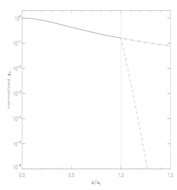
Schematic time-correlation (χ_k) versus normalized eddy frequency (ω / ω_E) at k = 5k₀ (i.e. in the inertial subrange such as k_d ≫ k > k₀), where k₀ = 6.28 × 10^-6 m^-1. Note that the value of k₀ does not influence the result. The solid line (resp. dashed triple dot line) correponds to the Lorentizan functional form of χ_k for ω < ω_E (resp. ω < ω_E). The dashed line corresponds to a Gaussian modeling (χ_k ∝ e ^{− (ω / ω_E)2}) of characteristic frequency ω_E. (we numerically verified that e ^{− (τ / τ_E)2} is a good approximation of Eq. (7), see also Sect. 3.2). We stress that the sharp decrease the functional form given by Eq. (7), in the temporal Fourier domain, then justifies to consider ω_E as a cut-off frequency. In other words, χ_k is computed according to Eq. (12).