| Issue |
A&A
Volume 522, November 2010
|
|
|---|---|---|
| Article Number | A113 | |
| Number of page(s) | 8 | |
| Section | Stellar structure and evolution | |
| DOI | https://doi.org/10.1051/0004-6361/201014856 | |
| Published online | 09 November 2010 | |
Photometric variability of the Herbig Ae star HD 37806⋆
1
Department of Astronomy and AstrophysicsUniversity of Toronto,
50 St. George St.,
Toronto,
Ontario,
M5S 3H4
Canada
e-mail: This email address is being protected from spambots. You need JavaScript enabled to view it.
2
Institut für Astronomie, Universität Wien,
Türkenschanzstrasse
17, 1180
Vienna,
Austria
e-mail: This email address is being protected from spambots. You need JavaScript enabled to view it.
; This email address is being protected from spambots. You need JavaScript enabled to view it.
; This email address is being protected from spambots. You need JavaScript enabled to view it.
; This email address is being protected from spambots. You need JavaScript enabled to view it.
3
Warsaw University, Astronomical Observatory,
Al. Ujazdowskie 4,
00–478
Warszawa,
Poland
e-mail: This email address is being protected from spambots. You need JavaScript enabled to view it.
4
Department of Physics and Astronomy, University of British
Columbia, 6224 Agricultural Road,
Vancouver, BC
V6T 1Z1,
Canada
e-mail: This email address is being protected from spambots. You need JavaScript enabled to view it.
5
Department of Astronomy and Physics, St. Mary’s
University, Halifax, NS
B3H 3C3,
Canada
e-mail: This email address is being protected from spambots. You need JavaScript enabled to view it.
6
Départment de physique, Université de Montréal,
C.P. 6128,
Succ. Centre-Ville, Montréal,
QC
H3C 3J7,
Canada
e-mail: This email address is being protected from spambots. You need JavaScript enabled to view it.
7
Harvard-Smithsonian Center for Astrophysics, 60 Garden Street,
Cambridge,
MA
02138,
USA
e-mail: This email address is being protected from spambots. You need JavaScript enabled to view it.
Received: 23 April 2010
Accepted: 10 August 2010
Abstract
Context. The more massive counterparts of T Tauri stars, the Herbig Ae/Be stars, are known to vary in a complex way with no variability mechanism clearly identified.
Aims. We attempt to characterize the optical variability of HD 37806 (MWC 120) on time scales ranging between minutes and several years.
Methods. A continuous, one-minute resolution, 21 day-long sequence of MOST (Microvariability & Oscillations of STars) satellite observations has been analyzed using wavelet, scalegram and dispersion analysis tools. The MOST data have been augmented by sparse observations over 9 seasons from ASAS (All Sky Automated Survey), by previously non-analyzed ESO (European Southern Observatory) data partly covering 3 seasons and by archival measurements dating back half a century ago.
Results. Mutually superimposed flares or accretion instabilities grow in size from about 0.0003 of the mean flux on a time scale of minutes to a peak-to-peak range of < 0.05 on a time scale of a few years. The resulting variability has properties of stochastic “red” noise, whose self-similar characteristics are very similar to those observed in cataclysmic binary stars, but with much longer characteristic time scales of hours to days (rather than minutes) and with amplitudes which appear to cease growing in size on time scales of tens of years. In addition to chaotic brightness variations combined with stochastic noise, the MOST data show a weakly defined cyclic signal with a period of about 1.5 days, which may correspond to the rotation of the star.
Key words: stars: variables: T Tauri, Herbig Ae/Be / stars: individual: HD 37806 / techniques: photometric
Based on data from the MOST satellite, a Canadian Space Agency mission jointly operated by Dynacon Inc., the University of Toronto Institute for Aerospace Studies and the University of British Columbia, with the assistance of the University of Vienna, and on data from the All Sky Automated Survey (ASAS) conducted by the Warsaw University Observatory, Warsaw, Poland at the Las Campanas Observatory, Chile.
© ESO, 2010
1. Introduction
HD 37806 (SAO 132452, RA(2000) = 05:41:02.3, Dec(2000) = − 02:43:01, V ≃ 7.95) is an early star in the field of Sigma Ori. It is frequently referred to as MWC 120, the designation in the Merrill & Burwell Catalog (1933) of early type stars with emission lines, which it received following the discovery of Merrill et al. (1932). HD 37806 is a Herbig Ae/Be-type object, i.e. a young star which is more massive (typically 1.5 − 5M⊙) than solar and sub-solar mass T Tauri stars. The review of Waters & Waelkens (1998) summarizes the properties of Herbig Ae/Be-type stars; a catalogue of Herbig Ae/Be-type objects was published by Thé et al. 1994). The MK spectral type of HD 37806 is variously given as A2Vpe or B9Ve+sh (Swings & Struve 1943, Guetter 1981, Thé et al. 1994) although sometimes it is still quoted as A0. HD 37806 was one of the first “radio” stars identified (Feldman et al. 1973).
The age and cluster membership of HD 37806 are not well known, although the star does appear very young. While it is only 35 arcmin from Sigma Orionis, it was not included among the members of the young cluster carrying the name of this star in the study by Sherry et al. (2004; 2008). The distance estimated for the cluster, 420 ± 30 pc, is consistent with the Hipparcos new-reduction parallax 2.05 ± 0.91 mas (van Leeuwen 2007). The star almost certainly belongs to the Orion OB1b association (of which the Sigma Ori cluster may be a part), whose age is estimated at 2–5 Myr (Brown et al. 1994) and for which the Hipparcos group distance is  pc. In Brown et al. (1994), the distance to HD 37806 was estimated at about 300 pc, assuming V = 7.94, MV = + 0.2, and a moderately large AV = 0.35; for the Sigma Ori cluster, Sherry et al. (2004; 2008) estimate AV at about 0.1 to 0.2. The distance, the possible membership of HD 37806 to the Sigma Ori cluster and the amount of interstellar absorption all appear to be very uncertain at this point.
The main thrust of this paper is limited to utilizing the continuous, 21 day long observations by the MOST satellite for characterization of the optical variability of HD 37806. As auxiliary data, we use lower accuracy ESO and ASAS observations, which extend the time coverage to several years, and archival observations extending the time baseline to half a century. The data analysis tools are similar to those used for continuous MOST satellite observations of the T Tauri type star TW Hya (Rucinski et al. 2008).
The literature on diversified studies of HD 37806 in various spectral regions is extensive, where the star is usually identified by its more popular alias MWC 120. Among the recent studies, Mottram et al. (2007) pointed out that Herbig Ae stars (A0–A2), such as HD 37806, appear to be more similar in terms of the accretion processes producing the emission spectra to T Tauri stars than to earlier (B0–B3) Herbig Be stars. The star has also been the subject of extensive spectroscopic, polarimetric and spectro-polarimetric investigations (Vink et al. 2005). Of relevance to variability studies of HD 37806 is the finding by Harrington & Kuhn (2009) that the Hα line shows strong morphological changes on a time scale of 3 years.
Very recently, using a novel method of spectro-astrometric signatures, Wheelwright et al. (2010) found that HD 37806 is a binary system, similarly to the majority of surveyed 45 Herbig Ae/Be stars. This is a very important discovery which may provide the key explanation of the variability characteristics which we see in our MOST data; we return to this subject in Sects. 4 and 5.
2. Optical variability: Previous photometric results
2.1. Archival data
HD 37806 was observed in the Johnson V and Strömgren y (transformed to V) bands in 1959–1962 and 1968 by Hardie et al. (1964) and Warren & Hesser (1977). Additionally, de Winter et al. (2001) observed the star in 1986 and 1992. Although all these were few (2 and 5) scattered observations, they give an interesting constraint on the long term variability of the star (Sect. 4).
2.2. Hipparcos observations
Hipparcos satellite observations of 44 Herbig Ae/Be stars, obtained over 37 months of the mission in the Hp band, were analyzed by van den Ancker (1998). Typically a hundred time-dispersed HP magnitude determinations per star were obtained with accuracy of 0.008–0.015 mag. In this study, HD 37806 was observed to vary by about 0.07 mag. However, this study was obviously unable to define detailed variability characteristics of the star.
We looked at the Hipparcos data again. The data consist of 135 HP observations and 209 VT and BT observations of the Tycho project, the latter with rather large uncertainties of typically 0.06–0.12 mag. All observations tend to be strongly bunched in time as a result of the sky scanning pattern of the satellite and appear in only a few groups over the mission duration. The strong bunching would not be a detrimental obstacle for use in the long time-scale variability considerations, as in Sect. 4, if the main-project data were in the V rather than HP system.
In the end, we used only the Tycho-2 (Høg et al. 2000) well-calibrated, single data point corresponding to the average V = 7.934 ± 0.016 (note that there exists no Tycho-2 epoch photometry). It has been added to the remaining archival observations discussed later on (Sect. 4) in an attempt to relate variability seen in by us to its possible long-term continuation.
2.3. ESO observations
Four-color Strömgren uvby observations of HD 37806 were conducted at the European Southern Observatory (ESO) in 1985–1986 by several observers (Manfroid et al. 1991); the observations do not appear to have been analyzed so far. Altogether 55 observations in the y ( = V) band were obtained, with 12 during the first season of January – February 1985, 41 observations during the November 1985 – March 1986 season and with 2 observations in September 1986. The typical interval between observations was 2 days and there were no multiple observations taken on the same night. The observations were done differentially and were relatively accurate with typical measurement errors of 0.007 mag.
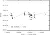 |
Fig. 1 The ESO light curve of HD 37806 in 3 seasons of 1985–1986, expressed in units of the mean flux. The central grouping of points corresponds to one Chilean observing season; the two other seasons were poorly covered. The HJD offset used in this figure is the same as for the remaining plots in this paper, hence the negative values of time. |
The ESO observations of HD 37806 are shown in Fig. 1. The observations do not indicate any regularity in its variability, but rather random noise, perhaps with increasing amplitudes for time scales ranging from single days to hundreds of days. We discuss the optical flux scatter in Sect. 3.3, where we interpret the variations in terms of stochastic noise characterized by  , where the observational (instrumental) noise is described by the contribution σR = 0.007.
2.4. ASAS observations
ASAS, the All Sky Automated Survey (Pojmański 1997; 2002; 2004; 2005; 20061), is a long term project dedicated to detection and monitoring of variability of bright stars using small telescopes. It has been run for a decade by Warsaw University at Las Campanas Observatory in Chile using 7 cm telescopes providing photometry in the 8–13 mag range. About three fourths of the sky ( − 90° < δ < + 28°) is covered on a regular basis.
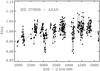 |
Fig. 2 The ASAS light curve of HD 37806 expressed in units of the mean flux. The groupings of points correspond to individual observing seasons. Note the different horizontal scale compared with Fig. 1. |
The ASAS observations of HD 37806, 424 in number, were obtained in the V filter over 9 seasons, from February 2001 to December 2009. They are shown in Fig. 2. The typical random errors are somewhat difficult to characterize and were typically at the level of 0.015–0.02 mag. The errors include a major component resulting from reductions of individual frames to the V band, which are done relative to all available Tycho-2 catalogue stars within the field of view of the telescope. While this approach assures the photometrically differential nature of the data (with possible systematic errors within the frame), it may generate – due to environmental factors such as clouds crossing the large field of view, extinction anomalies – random errors when individual frames are compared, as in variability studies. Also, the inexpensive (engineering grade CCD) detector had many bad and warm pixels which were observed to vary their response in time and were sometimes not immediately recognized in automatic reductions. These issues, coupled with the rather small variability amplitude for HD 37806 forced re-reductions of the data for this star which are slightly different from those available from the automatic on-line ASAS data system.
The observed brightness variations of HD 37806 are dominated by random stellar flux fluctuations, enlarged by the observational noise. In the analysis of the brightness fluctuations in Sect. 3.3 we assume observational random noise of σR = 0.017. The two well defined brightness decreases (at time 3050 and 4100 in Fig. 2) appear genuine as we could not identify any instrumental effects to produce them; they may be manifestations of sudden obscuration brightness drops observed for the UX Ori-type subclass of Herbig Ae/Be stars (Waters & Waelkens 1998).
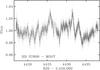 |
Fig. 3 The MOST light curve of HD 37806, covering 21 days, expressed in units of the mean flux, with one-minute sampling. The first half of the run experienced gaps of about 30% of each 103 min satellite orbit due to a high background level. The data set has been used at the full one-minute resolution as well as at the uniform, MOST-orbit time sampling necessary for the wavelet analysis (see Sect. 3.2.) |
3. MOST satellite observations
3.1. The data
Originally planned for two years, the MOST satellite has been observing variability of stars highly successfully since 2003. The optical system of the satellite consists of a Rumak-Maksutov f/6 15 cm reflecting telescope. The custom broad-band filter covers the spectral range of 380–700 nm with effective wavelength located close to Johnson’s V band. The pre-launch characteristics of the mission are described by Walker et al. (2003) and the initial post-launch performance by Matthews et al. (2004).
HD 37806 was observed by MOST in Guide Star mode for 21 days, during observations of Sigma Orionis and its surrounding stars in November 2007 (Townsend et al., in prep.). The data were reduced with other stars of this campaign using the MOST Guide Star Photometry reduction method (Hareter et al. 2008) and expressed as added counts per one minute interval. In this paper we utilize only the flux values corresponding to counts normalized to their mean value. The mean count rates are not relevant for error estimation because of the highly non-Poissonian noise characteristics resulting from addition of frequent CCD readouts (typically every second) of the Guide Star mode observations.
Continuous, uninterrupted, one-minute interval observations were done during the second half of the run. Thus, a full analysis at this temporal resolution could be done over a shorter interval of 9.5 days only (Sect. 3.3). During the first half of the run, the observations had stray-light elimination gaps of typically 29 min per 103 min MOST orbit. In this paper, we used both the whole dataset sampled at one minute as well as “normal points” obtained by median averaging of naturally formed groups of observations at MOST-orbit intervals of 0.07 d. The orbital normal points were used for the wavelet analysis (Sect. 3.2) which requires data sampled at strictly equidistant points in time.
Well-defined fluctuations of a few percent from the mean flux are visible in the MOST light curve (Fig. 3). The fluctuations appear to be reminiscent of flares or irregular brightening events observed in cataclysmic and nova-like variables (CV) and which are explained as stochastic variability resulting from superposition of overlapping accretion instability events in the disk surrounding the star.
Fourier analysis of the MOST data was done for all available data sampled at one minute intervals by fitting cosine-sine pairs with frequencies incremented in small steps to cover the whole accessible frequency range. This corresponded to a range extending from the lowest accessible 0.05 cycles per day (c/d) to several hundred cycles per day. The amplitude spectrum, shown in Fig. 4 in logarithmic units, is dominated by low-frequency variability at frequencies below a few cycles per day. Usually, due to stray-light effects, passages through the South Atlantic Anomaly, etc. the MOST orbit frequency of 14.2 c/d, along with a frequency of 1 c/d appear in such spectra but both are absent in the reduced material, attesting to good processing of the raw data. The low frequency content has led us to use in the wavelet analysis (Sect. 3.2) the data averaged into points sampled at the MOST-orbit frequency, i.e. below 7 c/d.
In addition to the Fourier component amplitudes, Fig. 4 gives the mean standard errors for the amplitudes, estimated using a bootstrap experiment of multiply re-sampled data. The errors start to become significant for frequencies higher than a few c/d; their value was used to estimate the average mean random error for the MOST data at σR = 0.0028 of the mean flux.
No coherent, periodic signal is visible in the amplitude spectrum except for a somewhat complex feature at about 0.65 c/d. The overall spectrum appears to be that of red stochastic noise, possibly even “redder” (with stronger low frequencies) than the common “flicker noise” (amplitudes scaling as  ; Press 1978); the slope of the amplitude spectrum may in fact show a change around the discrete spectral feature at ≃ 0.65 c/d or the period about 1.5 days (see Fig. 4).
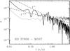 |
Fig. 4 The amplitude spectrum of the MOST variability data for HD 37806 is shown by the continuous line. The dotted line gives the Fourier amplitude errors estimated by a bootstrap re-sampling experiment. The broken lines, shown to guide the eye, give the slopes of a ∝ 1 / f and |
3.2. Wavelet transforms
The data for the wavelet transform must be arranged into a strictly equidistant time sequence to accommodate progressive extension of the temporal scale by integer multiples of the basic sampling interval. For MOST data, the most obvious such sampling interval is the duration of one satellite orbit around the Earth. Indeed, the majority of instrumental and stray-light problems usually manifest themselves with a period of 0.07046 d. The median flux values for HD 37806 from individual satellite orbits were obtained from typically 70 to 100 data points per median in the first half of the run (when orbital gaps were present) and up to 102 points (minus outliers and glitches) per median in the second half (the last 9.5 days) of the run. The resulting data were additionally spline interpolated – with very slight shifts of less than a minute – into a strictly equidistant time grid with steps of 0.07046 d. Two gaps in the mean data were present on HJD – 2 450 000 days 4427 and 4437; they were filled by spline interpolated points to obtain a uniform sequence of 301 data points.
Wavelet analysis is normally done with time-scale incremented as a power of 2, i.e. in 2, 4, 8, 16... data sampling intervals (here 0.07046 d each). The same sequence was used here, but – for convenience of the subsequent transform gray-scale displays – the scales were later interpolated into a linear sequence extending from 0.14 to 4 days; for still longer time scales, edge effects start becoming important for the MOST data.
Various types of wavelet functions are in widespread use in data processing (Torrence & Compo 1998). Selection of a particular type depends on the type of variability. The simplest and most often used are the Morlet wavelet of a sine-cosine pair confined in a Gaussian wave “packet”, which is useful for detection of short-lasting or evolving periodic events, and the Derivative of a Gaussian (DOG) wavelet, in its lowest-order version (the second derivative, DOG-2), which is sometimes called the Mexican Hat wavelet and which is useful for characterization of chaotic, localized events. We used both because variability of HD 37806 appears to be dominated by random, chaotically occurring flares, yet the lesson of TW Hya (Rucinski et al. 2008) taught us that such stars may show hidden, evolving periodicities. For the Morlet wavelet, we used the 6-th order version because it was found in the analysis of TW Hya that the more commonly used Morlet-5 did not reproduce the Fourier frequencies sufficiently well (and this has been confirmed again here); qualitatively, the results for both Morlet transforms are very similar.
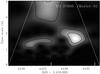 |
Fig. 5 The Morlet-6 wavelet (sine-cosine pair extending over 6 cycles and confined by a Gaussian) applied to the HD 37806 data sampled at the MOST orbital period of 0.07046 d. The light gray areas correspond to stronger power. Edge effects influence the wavelet transform beyond the broken lines. Note that the phase information for this complex-function transform has been disregarded by using the power of the transform. The missing orbital data were interpolated at two points marked by tick marks along the lower horizontal axis, but no detrimental effects appear to be present there. |
The Morlet-6 transform (Fig. 5) confirms the presence of a quasi-periodic signal with a period of about 1.5 d, which was already noted in the Fourier analysis (Fig. 4). In the wavelet transform, the 1.5 d signature appeared twice during the three weeks of the observations, with wavelet amplitudes 0.027 and 0.040 of the mean flux, which can be compared with the amplitude of a bit less than 0.003 in the whole, “diluted-in-time” Fourier spectrum. In Sect. 4 we interpret the 1.5 day period as related to the rotation of the star with Vsini = 120 ± 30 km s-1 (Boehm & Catala 1995).
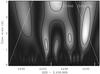 |
Fig. 6 The same as in Fig. 5, but for the DOG-2 wavelet (the negative second derivative of a Gaussian). Note that the shortest coherent noise structures seem to appear at time scales of about 0.25 d. |
The DOG-2 wavelet transform (Fig. 6), which is an excellent tool for studies of chaotic noise, shows a different picture from the Morlet-6 transform: We see individual brightening events which become larger for longer time scales. Some events die out quickly or may be just observational noise effects, but some grow in brightness for longer time scales. The growing strength with temporal scale is a characteristic feature for a self-similar noise process. This is discussed in the next section.
3.3. Brightness variability as stochastic noise
An underlying stochastic process is considered to be self-similar with similarity exponent α when it behaves as: X(λt) = λαX(t). Scargle et al. (1993) considered noise characteristics of accretion sources and introduced the concept of a “scalegram” function to measure the self-similarity properties of such processes. The same approach with an extensive discussion and utilization of wavelets for cataclysmic variable data appeared in Fritz & Bruch (1998). Indeed, the scalegram is particularly conveniently implemented using the wavelet transform results: in practice, it is the wavelet-summed power for progressively increased time scales as they change along the vertical axis in Figs. 5 or 6. With N points of input data, for the scale (number of equidistant data intervals) incremented as S = 2,4,8,..., the scalegram V(S) for the scale S is defined as: 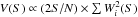 , where Wi(S) are the individual wavelet transform components for a given scale. If V(S) shows a linear behaviour in logarithmic units corresponding to V(S) ∝ S2α, then the underlying process is considered to be self-similar with exponent α.
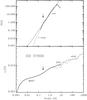 |
Fig. 7 Upper panel: The scalegram for the 21 days of the MOST data for HD 37806 based on the DOG-2 wavelet (continuous line) for the data were sampled at the MOST orbital period of 0.07 d. The horizontal axis gives the time scale in days. Because only slope values and their changes are important here, the vertical scale has an arbitrary zero point. The broken line has slope 3 in log–log units. The dotted line gives the scalegram for the shortest time scales, based on 9.5 days of data sampled at one-minute intervals (see Fig. 8); it has been shifted vertically to match the results for the coarsely sampled data. The arrow points at time scales where visual inspection suggests appearance of coherent structures in the DOG-2 wavelet transform. Lower panel: The continuous line gives the median standard deviation σ ⋆ for the full set of the MOST data (sampled at one minute), calculated for progressively longer time scales and corrected for the observational random error of σR = 0.0028, as described in the text. The dotted and broken lines give the ESO and the ASAS median dispersions at a given scale, corrected for observational errors σR of 0.007 and 0.017, respectively. |
For HD 37806, the DOG-2 wavelet transform appears to provide the best description of isolated and/or superimposed flares. In Fig. 6 we directly see the intensifying wavelet strength in the upward direction, towards longer scales. When expressed as the scalegram in log-log units (Fig. 7, the upper panel), the progression takes the shape of a linear dependence on time scales ranging approximately between 0.25 days and 4 days. For the MOST-orbit averaged data, the shorter time scales (shorter than the MOST orbit length) are not accessible, while scales longer than about 4–5 days become affected by edge effects of the full data sequence. Within the accessible range, the logarithmic slope appears to be about 3 (not a formal fit, just a rough approximation), so that the noise process is characterized by the exponent α ≃ 1.5. The sign and the magnitude of the exponent mean that longer noise events are stronger in intensity. Of course, any process with α > 0 has such a property, but we note that this particular value of the exponent is identical to that seen by Fritz & Bruch (1998) in many cataclysmic variables. However, for HD 37806, the time scales involved are hours and days rather than minutes as observed in CV’s.
The MOST-orbit frequency sampling of the data at 0.07 d sets an obvious limitation for the shortest time scales. This could be partly remedied by using the second half, 9.5 days long portion of the MOST observations which were obtained at one minute intervals without repeated scattered-light gaps. Still, even for this sequence, some data dropouts were present resulting in 97% temporal coverage; those single, occasional gaps were filled by spline interpolated points. The DOG-2 wavelet transform looks very different without any obvious indication of growing, coherent structures (Fig. 8). The small features which we do see can be explained by minor instrumental discontinuities and other data imperfections which became relatively more important when the fluctuations in stellar flux were very small.
The wavelet transform and the related scalegram are excellent tools in defining the temporal scales and the noise-strength progression with scale. But the size or strength of the fluctuations is difficult to gauge. To relate the scalegram results to the observed data scatter measured by the standard mean error σobs, a simple analysis of the scatter was done for the whole available MOST dataset: values of the mean standard error σobs were calculated along the time sequence for increased scales (intervals) starting at single minutes and ending at 10 days, making sure that each interval had a meaningful number of at least 5 points. Then, for each scale S, the median σmed(S) value was found from all individual values of σobs as a characteristic noise number for that scale. Although very simple, this approach has led to surprisingly well defined values of the typical fluctuations as they varied with the length of the interval. The results are plotted in the lower panel of Fig. 7 after being corrected for the observational random error σR as 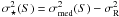 . The assumption for the MOST data was that σR = 0.0028 as estimated for the shortest scales and in agreement with the expected observational random error at V ≃ 8. The results confirm the scalegram progression and may even confirm that a change in the noise characteristics was present around 0.25 days.
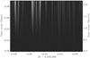 |
Fig. 8 The DOG-2 wavelet applied to the HD 37806 data sampled at one minute intervals during the second half of the MOST observations. Note the qualitatively different picture from that in Fig. 6. |
The same procedure of the  determination as for the MOST data was repeated for the longer but more poorly sampled ESO data (Sect. 2.3 and Fig. 1) and the ASAS data (Sect. 2.4 and Fig. 2). The MOST and the ground-based results appear to agree very well and overlap in Fig. 7 for the stated observational error of the ESO observations of σR = 0.007. For the ASAS observations the error has been assumed to be σR = 0.017, which is a less well defined number but agrees with the typical accuracy of 0.015 to 0.02 mag. The brightness fluctuations of HD 37806 appear to grow in size up to the accessible scales of some two thousand days, confirming the “red-noise” characteristics of the variability.
4. Discussion and interpretation
Because of the lack of spectroscopic support, our data cannot unequivocally determine the cause of variability of HD 37806. Some guidance can be found in extensive recent results for T Tauri stars to which Herbig Ae stars appear to be more similar in terms of their activity than to Herbig Be stars (Mottram et al. 2007). Of various processes identified in T Tauri stars (Bertout et al. 1988; Bertout 1989; Bouvier et al. 2007), one may consider: (1) photospheric spot rotational modulation; (2) variable obscuration by the dusty accretion disk; (3) instabilities in the accretion shock funnel on the stellar surface; (4) instabilities in the accretion disk. In addition, Herbig Ae stars appear within the δ Sct instability strip so that pulsations are also possible.
The wavelet analysis tells us that variability of HD 37806 takes the form of upward-directed spikes, rather than dimming events. This suggests that it is caused by accretion instabilities on the surface or in the space adjacent to the star. Rich and complex accretion phenomena in young stars have been thoroughly described in the monograph of Hartmann (2009). While considered by us as the most likely process from the start, the accretion explanation has recently found a very strong support in the discovery of Wheelwright et al. (2010) that the star is a binary system. This discovery needs confirmation as the angular separation is relatively small for the method used, 0.025 ± 0.001 arcsec, and the data for HD 37806 are of moderate quality. The implied physical separation of components for the distance of 300–500 pc is of the order of 0.7–1.0 AU indicating that the accretion process involves relatively large spatial dimensions; this would agree with our results that the red-noise variability extends to temporal time scales as long as several years (see below).
An explanation of the observed variability of HD 37806 by stellar pulsations does not seem to be viable. Light variations of HD 37806 in no way resemble stellar pulsations observed for another Herbig Ae star HD 142666, which was also observed by MOST (Zwintz et al. 2009). Also, HD 37806 is hotter than the hot edge of the classical Delta Scuti instability strip. Still, we carefully analyzed the MOST data for HD 37806 in the frequency range where δ Scuti-like pulsations would be expected, i.e. for frequencies between 5 and 80 c/d or periods between about 5 h and 20 min. The only detectable, significant peaks in the amplitude spectrum can be attributed to the instrumentally induced frequencies which are well characterized for the MOST data.
The quasi-periodic signal with a period of about 1.5 d, which is visible in the Fourier (Fig. 4) as well as in the Morlet transform (Fig. 5), finds the simplest explanation in an accretion area periodically brought into view by rotation of the star. Note, that this appears to be a bright, weakly-defined signature rather than one corresponding to a dark, sunspot-like feature. The observed Vsini = 120 ± 30 km s-1 (Boehm & Catala 1995) can be reproduced for this period – assuming rigid rotation – by R = (3.5 ± 0.8R⊙) / sini.
The main finding of this work of self-similar brightening events combining into chaotic red-noise (Figs. 6 and 7) may be interpreted as manifestations of instabilities in an accretion disk around the star with progressively larger areas of the accretion disk producing longer-lasting events. The instabilities produce undetectable ( < 0.0003 of the mean flux) variations for time scales of minutes, become very well defined (at about 0.003 of the mean flux) for time scales of hours, grow to ≃ 0.010 of the mean flux at time scales of 1–10 days and continue increasing for time scales of weeks to a few years where they reach 0.025 of the mean flux (see Fig. 7). Although these variations are very well visible and characterized thanks to the good quality of the observations, they remain relatively small, indicating that the star dominates in the mean brightness.
If interpreted by circumstellar events with time scales dynamically related to sizes, for a 3M⊙ star, dimensions corresponding to scales of hours to years would range between a fraction of a stellar radius to ≃ 3 AU. Such a range of dimensions may correspond to an accretion disk similar to those observed in T Tauri stars or one created by the matter falling from a close companion. The interferometric observations of Eisner et al. (2004) did not rule out the presence of a binary companion at < 1 AU and were unable to determine the inclination of the circumstellar material around the star. The new spectro-astrometric method of Wheelwright et al. (2010) did detect a companion at ≤ 1 AU, but the detection is rather preliminary and requires confirmation.
Does the red-noise variability keep on growing at time scales longer than 9 years covered by the ASAS (Sect. 2.4) project? A comparison of V magnitudes obtained from various sources (Sect. 2.1) and extending over about half a century, is shown in Fig. 9. Although the data are of a somewhat non-uniform quality, there is a clear indication that variations of HD 37806 are apparently small, not exceeding ± 0.05 of the mean flux, which is not much more than accuracy of some of the early observations. The small spread in the measured V magnitudes is in fact surprising taking into account that some of the archival observations were transformed from the y-band of the ubvy photometry and that the star is an emission-line object; both circumstances might have easily increased the observational scatter through problems of photometric transformations. We note that the only indication of systematic changes is the presence of a small brightness decrease which may have taken place sometime between 1995 and 2000.
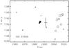 |
Fig. 9 V-band magnitudes of HD 37806 from the literature (Hardie et al. 1964; Warren & Hesser 1977; de Winter et al. 2001, see Sect. 2.1; crosses), ESO (Manfroid et al. 1991, see Sect. 2.3; filled circles) and ASAS (Sect. 2.4; open circles) with sizes of symbols logarithmically scaled depending on the number of data points in a given season (compare with Figs. 1 and 2). While the literature plotted data correspond to typically 2–5 observations obtained within a few days, the ESO and ASAS observations correspond up to 80 observations per season. The large cross marks the mean Tycho-2 V magnitude with its uncertainty assigned here for the duration of the Hipparcos mission. |
5. Summary
Although the Herbig Ae/Be star HD 37806 was a secondary object during the MOST observations of the Sigma Ori field, the results may be of primary importance to studies of variability of these young, massive stars. Variability of HD 37806 appears to be similar in general characteristics to that of the T Tauri star TW Hya (Rucinski et al. 2008) in that both stars – observed by MOST and analyzed in a similar way – showed brightness fluctuations apparently due to instabilities in the matter accretion process. An accretion disk may be fed by circumstellar matter or – in the case of HD 37806 – most likely by a companion. The process is unstable and produces progressively larger variability amplitudes at longer temporal scales, a property which can be characterized as “red noise”.
The variations in TW Hya and HD 37806 differ in terms of temporal as well as magnitude of variations. For TW Hya, the red noise contained discrete, relatively large (typically 0.1–0.2 of the mean flux), periodic variations lasting typically a couple of weeks. They evolved in their period-length towards shorter periods (a well defined variation evolved from about 6 days to 3 days in three weeks and another appeared at about 7 days). For HD 37806, variations are much smaller (typically 0.01–0.02 of the mean flux) which may reflect a much larger brightness of the star itself, and we see no indications of periodic components similarly drifting in period: A single, weak, periodic signature of about 1.5 days did not show any temporal evolution in time and may be related to inhomogeneities on this rapidly rotating star. However – importantly – brightening events of HD 37806 showed clear self-similar characteristics, growing in intensity with time scale. The self-similar characteristics of stochastic variability were established for the time scale range of about 4 h to 4 days. The self-similarity exponent (α ≃ 1.5) of the noise was found to be very similar to that observed in cataclysmic variables at much shorter time scales of minutes. The similarity to the CV’s may be not accidental in view of the recent result of Wheelwright et al. (2010) that HD 37806 is most likely a binary with the component separation of ≤ 1 AU.
The archival data on the variability of HD 37806 suggest its continuation – with a possible moderation – for long time scales. The red noise characteristics do appear in a simple analysis of the typical (median) standard dispersion of the noise for progressively increased time scales. The large temporal and time-range extent of the combined MOST, ESO and ASAS data permits one to see a well defined progression in the amplitude – scale dependence up to intervals of a few years. The red-noise fluctuations grow for time scales ranging from minutes to a few years from below 0.0003 to 0.025 of the mean flux. The fragmentary and – by their nature – somewhat non-uniform archival V magnitude data do not suggest any drastic noise increase ( < 0.05) for still longer time scales extending to half of a century.
Acknowledgments
The Natural Sciences and Engineering Research Council of Canada supports the research of D.B.G., J.M.M., A.F.J.M., and S.M.R.; additional support for A.F.J.M. comes from FQRNT (Québec). R.K. and W.W.W. are supported by the Austrian Space Agency and the Austrian Science Fund. K.Z. acknowledges support by the Austrian Fonds zur Förderung der wissenschaftlichen Forschung (FWF; project T335-N16) and is recipient of an APART fellowship of the Austrian Academy of Sciences at the Institute of Astronomy of the University of Vienna. G.P. acknowledges support by the Polish MNiSW grant N203 007 31/1328. This research has made use of the SIMBAD database, operated at CDS, Strasbourg, France and NASA’s Astrophysics Data System (ADS) Bibliographic Services. We thank the reviewer for useful and constructive comments and suggestions.
References
- van den Ancker, M. E., de Winter, D., & Tjin A, Djie, H. R. E. 1998, A&A, 330, 145 [NASA ADS] [Google Scholar]
- Boehm, T., & Catala, C. 1995, A&A, 301, 155 [NASA ADS] [Google Scholar]
- Bertout, C. 1989, ARA&A, 27, 351 [NASA ADS] [CrossRef] [Google Scholar]
- Bertout, C., Basri, G., & Bouvier, J. 1988, ApJ, 330, 350 [NASA ADS] [CrossRef] [Google Scholar]
- Bouvier, J., Alencar, S. H. P., Boutelier, T., et al. 2007, A&A, 463, 1017 [NASA ADS] [CrossRef] [EDP Sciences] [Google Scholar]
- Brown, A. G. A., de Geus, E. J., & de Zeeuw, P. T. 1994, A&A, 289, 101 [NASA ADS] [Google Scholar]
- Eisner, J. A., Lane, B. F., Hillenbrand, L. A., et al. 2004, ApJ, 613, 1049 [NASA ADS] [CrossRef] [Google Scholar]
- Feldman, P. A., Purton, C. R., & Marsh, K. A. 1973, Nature Phys. Sci., 245, 7 [NASA ADS] [Google Scholar]
- Fritz, T., & Bruch, A. 1998, A&A, 332, 586 [NASA ADS] [Google Scholar]
- Guetter, H. H. 1981, AJ, 86, 1057 [NASA ADS] [CrossRef] [Google Scholar]
- Hardie, R. H., Heiser, A. M., & Tolbert, C. R. 1964, ApJ, 140, 1472 [NASA ADS] [CrossRef] [Google Scholar]
- Hareter, M., Reegen, P., Kuschnig, R., et al. 2008, CoAst, 156, 48 [NASA ADS] [CrossRef] [Google Scholar]
- Harrington, D. M., & Kuhn, J. R. 2009, ApJS, 180, 138 [NASA ADS] [CrossRef] [Google Scholar]
- Hartmann, L., 2009, Accretion Processes in Star Formation, (Cambridge University Press), 2nd edn. (1st Edn, 1998) [Google Scholar]
- Høg, E., Fabricius, C., Makarov, V. V., et al. 2000, A&A, 355, L27 [NASA ADS] [Google Scholar]
- van Leeuwen, F. 2007, Hipparcos, the New Reductions of the Raw Data; Astroph. Space Lib (Springer), 350 [Google Scholar]
- Manfroid, J., Sterken, C., Bruch, A., et al. 1991, A&AS, 87, 481 (ESO Sci. Rep., 8) [Google Scholar]
- Matthews, J. M., Kusching, R., Guenther, D. B., et al. 2004, Nature, 430, 51 [NASA ADS] [CrossRef] [PubMed] [Google Scholar]
- Merrill, P. W., & Burwell, C. G. 1933, ApJ, 78, 87 [NASA ADS] [CrossRef] [Google Scholar]
- Merrill, P. W., Humason, K. L., & Burwell, C. G. 1932, ApJ, 76, 156 [NASA ADS] [CrossRef] [Google Scholar]
- Mottram, J. C., Vink, J. S., Oudmaijer, R. D., & Patel, M. 2007, MNRAS, 377, 1363 [NASA ADS] [CrossRef] [Google Scholar]
- Paczyński, B., Szczygieł, D., Pilecki, B., & Pojmański, G. 2006, MNRAS, 368, 1311 [NASA ADS] [CrossRef] [Google Scholar]
- Perryman, M. A. C., Lindegren, L., Kovalevsky, J., et al. 1997, A&A, 323, L49 [NASA ADS] [Google Scholar]
- Pojmański, G. 1997, Acta Astron., 47, 467 [NASA ADS] [Google Scholar]
- Pojmański, G. 2002, Acta Astron., 52, 397 [NASA ADS] [Google Scholar]
- Pojmański, G. 2004, Astron. Nachr., 325, 553 [NASA ADS] [CrossRef] [Google Scholar]
- Pojmański, G., & Maciejewski, G. 2005, Acta Astr., 55, 97 [Google Scholar]
- Press, W. H. 1978, Comm. Astrophys., 7, 103 [Google Scholar]
- Rucinski, S. M., Matthews, J. M., Kuschnig, R., et al. 2008, MNRAS, 391, 1913 [NASA ADS] [CrossRef] [MathSciNet] [Google Scholar]
- Scargle, J. D., Steiman-Cameron, T., Young, K., et al. 1993, ApJ, 411, L91 [NASA ADS] [CrossRef] [Google Scholar]
- Sherry, W. H., Walter, F. M., & Wolk, S. J., 2004, ApJ, 128, 2316 [Google Scholar]
- Sherry, W. H., Walter, F. M., Wolk, S. J., & Adams, N. R. 2008, ApJ, 135, 1616 [Google Scholar]
- Swings, P., & Struve, O. 1943, ApJ, 98, 91 [NASA ADS] [CrossRef] [Google Scholar]
- Thé, P. S., de Winter, D., & Pérez, M. R. 1994, A&AS, 104, 315 [Google Scholar]
- Torrence, C., & Compo, G. P. 1998, Bull. Amer. Meteorological Soc., 79, 61 [NASA ADS] [CrossRef] [Google Scholar]
- Vink, J. S., Drew, J. E., Harries, T. J., Oudmaijer, R. D., & Unruh, Y. 2005, MNRAS, 359, 1049 [NASA ADS] [CrossRef] [Google Scholar]
- Walker, G., Matthews, J., Kuschnig, R., et al. 2003, PASP, 115, 1023 [NASA ADS] [CrossRef] [Google Scholar]
- Warren, W. H., & Hesser, J. E. 1977, ApJS, 34, 115 [NASA ADS] [CrossRef] [Google Scholar]
- Waters, L. B. F. M., & Waelkens, C. 1998, ARA&A, 36, 233 [NASA ADS] [CrossRef] [Google Scholar]
- Wheelwright, H. E., Oudmaijer, R. D., & Goodwin, S. P. 2010, MNRAS, 401, 1199 [NASA ADS] [CrossRef] [Google Scholar]
- de Winter, D., van den Ancker, M. E., Maira, A., et al. 2001, A&A, 380, 609 [NASA ADS] [CrossRef] [EDP Sciences] [Google Scholar]
- Zwintz, K., Kallinger, T., Guenther, D. B., et al. 2009, A&A, 494, 1031 [NASA ADS] [CrossRef] [EDP Sciences] [Google Scholar]
All Figures
|
Fig. 1 The ESO light curve of HD 37806 in 3 seasons of 1985–1986, expressed in units of the mean flux. The central grouping of points corresponds to one Chilean observing season; the two other seasons were poorly covered. The HJD offset used in this figure is the same as for the remaining plots in this paper, hence the negative values of time. |
| In the text | |
|
Fig. 2 The ASAS light curve of HD 37806 expressed in units of the mean flux. The groupings of points correspond to individual observing seasons. Note the different horizontal scale compared with Fig. 1. |
| In the text | |
|
Fig. 3 The MOST light curve of HD 37806, covering 21 days, expressed in units of the mean flux, with one-minute sampling. The first half of the run experienced gaps of about 30% of each 103 min satellite orbit due to a high background level. The data set has been used at the full one-minute resolution as well as at the uniform, MOST-orbit time sampling necessary for the wavelet analysis (see Sect. 3.2.) |
| In the text | |
|
Fig. 4 The amplitude spectrum of the MOST variability data for HD 37806 is shown by the continuous line. The dotted line gives the Fourier amplitude errors estimated by a bootstrap re-sampling experiment. The broken lines, shown to guide the eye, give the slopes of a ∝ 1 / f and |
| In the text | |
|
Fig. 5 The Morlet-6 wavelet (sine-cosine pair extending over 6 cycles and confined by a Gaussian) applied to the HD 37806 data sampled at the MOST orbital period of 0.07046 d. The light gray areas correspond to stronger power. Edge effects influence the wavelet transform beyond the broken lines. Note that the phase information for this complex-function transform has been disregarded by using the power of the transform. The missing orbital data were interpolated at two points marked by tick marks along the lower horizontal axis, but no detrimental effects appear to be present there. |
| In the text | |
|
Fig. 6 The same as in Fig. 5, but for the DOG-2 wavelet (the negative second derivative of a Gaussian). Note that the shortest coherent noise structures seem to appear at time scales of about 0.25 d. |
| In the text | |
|
Fig. 7 Upper panel: The scalegram for the 21 days of the MOST data for HD 37806 based on the DOG-2 wavelet (continuous line) for the data were sampled at the MOST orbital period of 0.07 d. The horizontal axis gives the time scale in days. Because only slope values and their changes are important here, the vertical scale has an arbitrary zero point. The broken line has slope 3 in log–log units. The dotted line gives the scalegram for the shortest time scales, based on 9.5 days of data sampled at one-minute intervals (see Fig. 8); it has been shifted vertically to match the results for the coarsely sampled data. The arrow points at time scales where visual inspection suggests appearance of coherent structures in the DOG-2 wavelet transform. Lower panel: The continuous line gives the median standard deviation σ ⋆ for the full set of the MOST data (sampled at one minute), calculated for progressively longer time scales and corrected for the observational random error of σR = 0.0028, as described in the text. The dotted and broken lines give the ESO and the ASAS median dispersions at a given scale, corrected for observational errors σR of 0.007 and 0.017, respectively. |
| In the text | |
|
Fig. 8 The DOG-2 wavelet applied to the HD 37806 data sampled at one minute intervals during the second half of the MOST observations. Note the qualitatively different picture from that in Fig. 6. |
| In the text | |
|
Fig. 9 V-band magnitudes of HD 37806 from the literature (Hardie et al. 1964; Warren & Hesser 1977; de Winter et al. 2001, see Sect. 2.1; crosses), ESO (Manfroid et al. 1991, see Sect. 2.3; filled circles) and ASAS (Sect. 2.4; open circles) with sizes of symbols logarithmically scaled depending on the number of data points in a given season (compare with Figs. 1 and 2). While the literature plotted data correspond to typically 2–5 observations obtained within a few days, the ESO and ASAS observations correspond up to 80 observations per season. The large cross marks the mean Tycho-2 V magnitude with its uncertainty assigned here for the duration of the Hipparcos mission. |
| In the text | |
Current usage metrics show cumulative count of Article Views (full-text article views including HTML views, PDF and ePub downloads, according to the available data) and Abstracts Views on Vision4Press platform.
Data correspond to usage on the plateform after 2015. The current usage metrics is available 48-96 hours after online publication and is updated daily on week days.
Initial download of the metrics may take a while.