| Issue |
A&A
Volume 522, November 2010
|
|
|---|---|---|
| Article Number | A81 | |
| Number of page(s) | 17 | |
| Section | Stellar structure and evolution | |
| DOI | https://doi.org/10.1051/0004-6361/201014769 | |
| Published online | 04 November 2010 | |
On detectability of Zeeman broadening in optical spectra of F- and G-dwarfs ⋆,⋆⋆
1
Observatoire de Genève, Université de Genève,
51 Ch. des Maillettes,
1290
Sauverny,
Switzerland
2
Institut für Astrophysik, Georg-August-Universität Göttingen, Friedrich-Hund-Platz
1, 37077
Göttingen,
Germany
3
Max-Planck-Institut für Sonnensystemforschung, Max-Planck-Straße
2, 37191
Katlenburg-Lindau,
Germany
4
School of Space Research, Kyung Hee University, Yongin,
Gyeonggi
446-701,
Korea
e-mail: This email address is being protected from spambots. You need JavaScript enabled to view it.
Received: 12 April 2010
Accepted: 11 August 2010
Abstract
We investigate the detectability of Zeeman broadening in optical Stokes I spectra of slowly rotating sun-like stars. To this end, we apply the LTE spectral line inversion package SPINOR to very-high quality CES data and explore how fit quality depends on the average magnetic field, Bf. One-component (OC) and two-component (TC) models are adopted. In OC models, the entire surface is assumed to be magnetic. Under this assumption, we determine formal 3σ upper limits on the average magnetic field of 200 G for the Sun, and 150 G for 61 Vir (G6V). Evidence for an average magnetic field of ~500 G is found for 59 Vir (G0V), and of ~1000 G for HD 68456 (F6V). A distinction between magnetic and non-magnetic regions is made in TC models, while assuming a homogeneous distribution of both components. In our TC inversions of 59 Vir, we investigate three cases: both components have equal temperatures; warm magnetic regions; cool magnetic regions. Our TC model with equal temperatures does not yield significant improvement over OC inversions for 59 Vir. The resulting Bf values are consistent for both. Fit quality is significantly improved, however, by using two components of different temperatures. The inversions for 59 Vir that assume different temperatures for the two components yield results consistent with 0−450 G at the formal 3σ confidence level. We thus find a model dependence of our analysis and demonstrate that the influence of an additional temperature component can dominate over the Zeeman broadening signature, at least in optical data. Previous comparable analyses that neglected effects due to multiple temperature components may be prone to the same ambiguities.
Key words: line: profiles / techniques: spectroscopic / Sun: surface magnetism / stars: late-type / stars: magnetic field
Based on observations collected at the European Southern Observatory, La Silla.
Appendix A is only available in electronic form at http://www.aanda.org
© ESO, 2010
1. Introduction
Cool stars display a range of phenomena that are typical of magnetic activity, such as dark spots present at the stellar surface (see Berdyugina 2005,for a review), enhanced chromospheric emission in, e.g., the Ca II H and K lines (e.g., Wilson 1994; Pizzolato et al. 2003; Hall & Lockwood 2004), flares (e.g., Favata et al. 2000; Maggio et al. 2000) and coronae (Schmitt 2001). Although these manifestations of stellar activity and hence of the underlying magnetic field are well detected for large samples of stars, measuring the magnetic field itself turns out to be difficult on most cool stars. The reason is the complex small-scale geometry of the field, that is amply evident on the Sun. The mixture of nearly equal amounts of magnetic flux of opposite polarities on the stellar disk leads to cancellation of the circular polarization signal due to the longitudinal Zeeman effect, the most straightforward diagnostic of a stellar magnetic field.
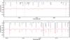 |
Fig. 1 Sample CES spectra illustrating data quality. Continua are shifted by ±0.3 from unity for visibility. Blue dash-dotted vertical lines indicate spectral lines used for analysis. Upper panel: data set A. Upper black spectrum: sunlight reflected from Jupiter’s moon Ganymede; lower red spectrum: HD 68456 (F6V, vsini ≈ 10 km s-1). Lower panel: data set B. Upper black spectrum: inactive and slow rotator 61 Vir (G6V); lower red spectrum: active and faster rotator 59 Vir (G0V, vsini ≈ 6.5 km s-1). |
Rapid stellar rotation partly removes the degeneracy between opposite magnetic polarities that lie sufficiently far apart on the stellar surface and thereby enables detection of a net (circular) polarization signal. Consequently, the magnetic field can be mapped on the stellar surface from the variation of the spectral shape and amplitude of this polarization signal over a stellar rotation, with the help of the Zeeman Doppler Imaging (ZDI) technique (Semel 1989), which has been successfully employed to reconstruct the large-scale distribution of the magnetic flux on the surfaces of a number of stars (Donati 2008; Donati & Landstreet 2009).
In spite of its success, ZDI does have some limitations. First, unless the field is homogeneously and unipolarly distributed on large scales, ZDI detects only some fraction of the true magnetic flux on the stellar surface. Second, the same is true for the measured field strength and hence the magnetic energy density. In general, the field strength is underestimated and consequently the magnetic energy density is even more strongly underestimated, since it is proportional to the square of the field strength (see Reiners & Basri 2009). Third, ZDI is limited to comparatively rapidly rotating stars. The slower a star rotates (or rather the smaller its vsini) the lower the spatial resolution of the stellar surface (and of the magnetic field) that can be achieved.
Therefore, the method proposed and applied to cool stars by Robinson (1980); Robinson et al. (1980), of looking for changes in the line profile shape of the intensity (Stokes I) due to Zeeman splitting, remains an interesting technique to complement ZDI. In particular, it allows an estimate of the total magnetic flux as well as of the field strength and filling factor to be obtained (and hence also of the magnetic energy density).
Zeeman broadening in stellar spectra (ZB) was first measured by Preston (1971) to determine the average surface magnetic fields of Ap stars. Robinson et al. (1980) then measured ZB in cool stars using his Fourier-based method which was taken up and extended by other authors (Gray 1984; Marcy 1982). It was soon realized, however, that the assumptions made in these Fourier techniques were too crude. Thus, a shift towards ever-improving forward radiative transfer calculations occurred. The development of these techniques was driven, among others, by Saar (1988, 1990b, 1996); Basri & Marcy (1988); Linsky et al. (1994); Rüedi et al. (1997); Johns-Krull & Valenti (2000).
The displacement of a circularly polarized σ-component from line center can be expressed by: ![Mathematical equation: \begin{equation} \Delta \lambda_{B} \approx 4.67 \times 10^{-13}\,g_{\rm{eff}}\,B\,\lambda^{2}\,\,\,[\AA]. \label{eq:ZeemanBroadening} \end{equation}](/articles/aa/full_html/2010/14/aa14769-10/aa14769-10-eq17.png) (1)For values typical of optical spectral lines, Eq. (1) demonstrates that even a comparatively strong field field along LOS is hard to detect. Bf = 1 kG would produce a Zeeman splitting of merely λB = 17 mÅ for the σ-components of a normal Zeeman triplet of a hypothetical line at 6000 Å with geff = 1.00, or λB = 42 mÅ in the case of a more sensitive geff = 2.50 line. This should be compared to the line width of a typical stellar line profile broadened thermally and due to turbulence by 2–6 km s-1 (i.e. 30–60 mÅ), as well as by rotation between 0 and 5 km s-1 (i.e. up to 100 mÅ). In addition, the resolution element at even very high resolving power, R, is comparable in size, e.g. δλ = 27 mÅ for R = 220000.
(1)For values typical of optical spectral lines, Eq. (1) demonstrates that even a comparatively strong field field along LOS is hard to detect. Bf = 1 kG would produce a Zeeman splitting of merely λB = 17 mÅ for the σ-components of a normal Zeeman triplet of a hypothetical line at 6000 Å with geff = 1.00, or λB = 42 mÅ in the case of a more sensitive geff = 2.50 line. This should be compared to the line width of a typical stellar line profile broadened thermally and due to turbulence by 2–6 km s-1 (i.e. 30–60 mÅ), as well as by rotation between 0 and 5 km s-1 (i.e. up to 100 mÅ). In addition, the resolution element at even very high resolving power, R, is comparable in size, e.g. δλ = 27 mÅ for R = 220000.
The present paper has a two-fold purpose. On the one hand, it is in the tradition of increasing the realism and accuracy of magnetic field measurements on cool stars. It applies state of the art inversion techniques to determine the magnetic field. Also, from observations of the Sun it is clear that magnetic fields are associated with significant brightenings or darkenings, which are generally neglected when measuring stellar magnetic fields. In the present paper we have carried out first simple computations looking at the effects that including such a diagnostic would have. We do not propose that this is an exhaustive or final study, but it can be considered as a first indicator. Finally, these techniques are also applied to spectral time series of an active star that has so far not been studied in this respect.
2. Data
2.1. Instruments and reduction
Spectra of the stars investigated were obtained with the Coudé Échelle Spectrometer (CES) at the 3.6 m ESO telescope at La Silla, Chile. This fiber-fed spectrometer achieved a spectral resolving power of approximately 220000 using an image-slicer and projecting only part of an order onto the CCD, resulting in a small wavelength coverage of approx. 40 Å.
Spectra from two data sets were used in this work: data set A, with 5770 < λ < 5810 Å, observed on 13 October 2000 (solar spectrum) and 2 October 2001 (HD 68456), and data set B, 6137 < λ < 6177 Å, observed on 7 May 2005 (HD 68456, 59 Vir). Sample spectra from both sets are shown in Fig. 1. We refer to Reiners & Schmitt (2003, hereafter R&S03) for more details, as data set A was originally taken for the project described in that publication.
Where necessary, continuum normalization corrections were performed by division of linear slopes fitted to the original continuum. Spectra were shifted to laboratory rest-wavelengths, by cross-correlation using the FTS solar atlas (Kurucz et al. 1984).
2.2. Objects, spectral lines, and atomic line information
In this work, we present results for 4 objects ranging in spectral type from F6V to G6V, including sunlight reflected from Ganymede (previously and hereafter referred to as the solar spectrum). These stars were especially suitable for our analysis for multiple reasons. First, identification of spectral line blends was facilitated in the effective temperature range covered by these stars and LTE atmospheres were readily available (Kurucz 1992). Second, the analysis of stars with relatively low projected rotational velocities, v sin i ≲ 10 km s-1, allowed us to fully exploit the high resolving power of the data and minimizes effects due to differential rotation. Third, measured stellar parameters such as effective temperature, Teff, surface gravity, log g and elemental abundances, [Fe/H] in particular, were available as constraints and could be directly input into the inversion procedure. Last, but not least, measured X-ray luminosities, LX, and previously reported magnetic field detections could be considered as indicators for the presence of magnetic fields (Saar 1990b) and thus helped to constrain the sample.
Within the small wavelength coverage of the CES spectra, only few relatively blend-free lines could be identified. Among these, we searched for combinations of lines that provide strong constraints on atmospheric properties. For instance, lines of different excitation potentials, χe, have different temperature sensitivities and often probe different heights (depending also on their equivalent widths). Therefore they constrain temperature stratification. In order to exploit the differential effect of Zeeman broadening, we aimed to cover the largest possible range in geff as well as to use the line with the greatest possible geff.
Most spectral lines could be identified in the postscript version of the FTS solar atlas available online. The remaining lines and blends were identified by searching the Vienna (Kupka et al. 2000, hereafter VALD) and Kurucz & Bell (1995) atomic line databases. These databases further provided the atomic line data, such as level configurations and log (g∗f∗) values required for the forward radiative transfer calculations, cf. Sect. 3. Effective Landé values, geff, were calculated from the atomic level configurations following Beckers (1969). The calculated effective and empirical Landé factors determined by Solanki & Stenflo (1985) were found to agree for all but one line: Fe I at 6165.36 Å, for which gemp = 0.69 and geff = 1.00. However, this line contains a blend at 6165.36 Å, for which geff = 0.67, cf. Table 1.
Spectral lines and their parameters used in inversions.
For some lines, ranges of log (g∗f∗) values were found in VALD. We aimed to determine the best log (g∗f∗) value for our selected lines by means of a by-hand gauging procedure using the solar spectrum for data set A and that of 61 Vir for data set B, while taking care to stay as close to the literature values as possible. This approach was adopted in order to avoid multiple additional free fit parameters, since one log (g∗f∗) for each blend would have been required. An automated approach would have been dominated by degeneracy between oscillator strengths and stellar model parameters.
Table 1 lists all lines used and parameters adopted in our inversions. Horizontal spacings help distinguish between blends contributing to the shape of a given spectral line and different lines. Column 1 lists abbreviations used in this paper for the respective line sets. Column 2 contains wavelength in Å. Column 3 the corresponding ion in spectroscopic notation, i.e. Fe I is neutral iron. Column 4 lists log (g∗f∗) adopted after gauging with the closest literature value in brackets, if a value outside the VALD range was adopted. Columns 5 and 6 contain excitation potential of the lower level of the transition, χe, and effective Landé factor, geff, respectively. The range in Landé factor covered by line set A3 is thus Δgeff = 1.08, and Δgeff = 1.50 for line sets B3 and B4, not counting blends. More importantly, the maximum geff is larger by 0.5 in line sets B3 and B4 than in line set A3. Therefore, a stronger sensitivity to ZB in the latter two data sets can be expected.
Collisional damping parameters are derived internally by SPINOR from cross-sections published by Anstee & O’Mara (1995); Barklem & O’Mara (1997); Barklem et al. (1998) and are not listed in the table.
Logarithmic elemental abundances adopted on scale where hydrogen equals 12.
Table 2 lists the elemental abundances adopted. Solar abundances used were those determined by Grevesse & Sauval (1998) and served as the absolute scale for relative stellar literature values found in Valenti & Fischer (2005, from hereon V&F05) (59 Vir & 61 Vir) and Cayrel de Strobel et al. (1997) (HD 68456).
Lines that correspond to elements for which no abundance measurements were found were usually not included in the inversions. For the Cr I line in A3 as well as some blends, e.g. Eu II in B3, abundances were estimated from an iterative fitting procedure that took into account published average metallicities. This procedure is potentially flawed, since general abundances are not necessarily correlated with individual abundances. However, this flaw does not challenge the work presented here, since Fe I lines were the most important ones for our analysis and literature values for iron were available for all stars. The Cr I line was of great importance only for the solar case, for which measurements of the chromium abundance (and also that of scandium) do exist. The blend due to Eu II was only of secondary significance, given its small impact on line shape. It was not discarded, however, since it provided continuum points for (at least the blue wing of) the Zeeman-sensitive 6173.3 Å line, for which the red wing was cut off due to the presence of unidentified blends.
One well known Zeeman sensitive line was omitted from the analysis, Fe II at 6149.24 Å. This line is very sensitive to magnetic fields due to its particular (doublet) Zeeman pattern, and displays clear Zeeman splitting in spectra of Ap stars (e.g. Mathys 1990; Mathys et al. 1997) and solar penumbrae (e.g. Lites et al. 1991). Unfortunately, this line is affected by blends in both line wings, as can be seen in Fig. 1 and we were not able to adequately reproduce these blended wings. While the blue wing blend is quite obvious, the red wing blend requires closer inspection. This blend is (at least in part) due to Ti I at 6149.73 Å and is hard to see due to rotational broadening, blending in with the smaller unidentified signatures seen in the slower rotator 61 Vir. This leads to the wing of the line just barely missing the continuum. Due to these two blended wings, the 6149.24 Å Fe II line profile used for inversion had either a badly defined continuum (the deviation from the continuum is around 1%), or lacked both line wings (if they were both cut off as was done for the red wing of the 6173 Å Fe II line) which meant not having any continuum points at all. Using either approach, we were not able to reach the same level of fit precision as presented for the other lines used in this analysis. Therefore, we chose to omit this line from our analysis.
Our results depend on the assumed Signal-to-Noise ratio (S/N), since (S/N)-1 = σi and 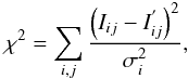 (2)where σi is significance, i line index, j data point index for a given line, Iij measured and
  calculated intensity normalized to the continuum value. We determined σi from the mean continuum standard deviation of the spectra. The typical S/N ratio thus determined was 400−700, corresponding to σ between 0.0025−0.00143. Less statistical weight was assigned to the pressure-sensitive Ca I line at 6162.18 Å by lowering significance to σ = 0.0040, since the wings of the line are heavily blended and asymmetric. Furthermore, the core of this line is affected by non-LTE effects and was therefore removed from the measured line profile.
In every line, we aimed to take full account of line blends and included as many data points reaching as far as possible into the continuum, since ZB affects the far line wings most strongly. However, some line wings had to be severed farther from continuum than others, since unidentified blends were present; see, for instance, the far red wing of the Zeeman-sensitive line at 6173.34 Å Fe I. This line wing showed strong contributions from at least one blend that could not be identified in line databases. To circumvent this problem, Rüedi et al. (1997) included fake iron blends until the line shape was matched. We chose not to introduce additional fit parameters, and instead decided to sever the far red line wing.
3. Analysis
We use spectral line inversion as the tool to explore detectability of ZB in this paper. Spectral line inversion denotes a combination of two things: forward radiative transfer calculations and an iterative non-linear least squares fitting process. In other words, spectral line profiles are calculated using a given atmospheric model and model parameters are iteratively adjusted until the highest possible agreement between calculated and observed spectral lines is reached. The resulting best-fit model parameters thus characterize the adopted atmospheric model and, if the model is assumed to be correct, the actual stellar atmosphere. Hence, we investigate whether introducing a magnetic field significantly improves the agreement between observed and calculated line profiles. We explain the general approach of spectral line inversion in the following subsection.
We further investigate model-dependence and the influence of model assumptions. To this end, two different kinds of models are used. These fitting strategies are documented in Sect. 3.2.
3.1. Spectral line inversions
We employ the spectral line inversion package SPINOR developed and maintained at ETH Zürich and MPS Katlenburg-Lindau for this analysis. In short, SPINOR computes synthetic intensity profiles (SIPs), L(λ), by solving the radiative transfer equation on a grid of optical depth points τ, accounting also for turbulence, rotation, magnetic fields, instrumental effects, etc. It then determines the model parameters used to compute L(λ) that best fit the observed data using a non-linear least squares fitting algorithm. We now briefly discuss how the SIPs used for inversion are calculated and refer to Frutiger et al. (2000, 2005, from hereon Fru00 and Fru05, respectively) for further information regarding SPINOR.
First, annular SIPs, I(λ,θ), are computed as a sum of weighted Voigt profiles (cf. Gray 2008, from hereon Gr08) combining thermal and pressure broadening, microturbulence (mass motions on a scale that is much smaller than the optical depth lead to a Doppler broadening due to a Gaussian velocity dispersion), vmic, and the full Zeeman pattern as described below. “Annular” here denotes the θ-dependence, since synthetic profiles are calculated for each of 15 concentric annuli that taken together approximate a flux profile resulting from a much larger number of intensity profiles at different viewing angles (Rüedi et al. 1997; Fru05). By calculating annular SIPs at different angular distances from disk center, we can include limb darkening due to its dependence on μ = cosθ.
To calculate the radiation transfer, we start with tabulated LTE atmospheres (Kurucz 1992). These atmospheres list the parameters temperature, pressure and electron pressure for a number of τ values and are calculated for given effective temperatures, Teff, and continuum opacity at 5000 Å. In general, the temperature values are allowed to vary in order to obtain an optimal fit to the spectral lines. Then, the whole temperature stratification T(τ) is shifted up or down. At each step in the inversion the atmosphere is always consistently maintained in hydrostatic equilibrium. Hence, from a prescribed temperature stratification, the gas and electronic pressures, the gas density and continuum opacity are computed assuming hydrostatic equilibrium. Note that temperature values returned by SPINOR correspond to unit optical depth calculated for continuum opacity at 5000Å.
The Zeeman shifts and amplitudes of the polarized components are calculated as explained in, e.g. Wittmann (1974). A detailed description of the implementation of the Zeeman effect in SPINOR can be found in Frutiger (2000, and references therein).
In a next step, the individual annular I(λ,θ) are convolved with radial-tangential macroturbulence profiles, Θ(λ,θ), that are intended to account for large-scale motion due to convection. These profiles are described in Gray (1975) and Gr08. Thus, we obtain new annular SIPs, I′(λ,θ) = I(λ,θ) ∗ Θ(λ,θ), where “∗” denotes convolution carried out as multiplication in Fourier space. In accordance with Fru05, we assume equal surface fractions covered by radial and tangential flows.
The radial velocities of individual surface elements vary across the stellar disk as a function of distance to the rotation axis, leading to rotational broadening in the integrated spectrum of a point source. This dependence is taken into account by introducing 15 new angles, φ, so that the radial velocity is constant at any given φ. Thus, the I′(λ,θ) are turned into I′(λ,θ,φ) and each one is shifted for radial velocity. The disk-integrated line profiles are obtained by weighting the individual I′(λ,θ,φ) for surface coverage, and summing up.
We obtain the final SIP, L(λ), by computing L(λ) = I′(λ) ∗ Iinst, that is by convolution of I′(λ) with an instrumental broadening function, Iinst. Iinst is a Gaussian function with a FWHM defined as a velocity, vinst, in km s-1 that corresponds to the resolving power of CES. Hence, we have R = 220000 = λ/Δλ = c/vinst. Therefore, for CES, vinst = 1.36kms-1.
Summing up, our model parameters are: temperature T1 (and T2 for two-component inversions, cf. Sect. 3.2.2), in Kelvin at unit optical depth; surface gravity log g in cgs units; projected rotational (vsini), microturbulent (vmic) and macroturbulent (vmac) velocities, each in km s-1. log g was kept fixed at literature values in most inversions, since narrow Fe I lines do not provide strong constraints on surface gravity. Inversions of line set B4, however, allowed log g to vary, since the pressure-sensitive Ca I line did provide this constraint. Finally, lines were allowed to be shifted in velocity space by ≤ 500 m s-1 (~0.01 Å at 6000 Å) to correct for slight differences in literature and data line center wavelengths, as well as possible shortcomings in the dispersion relation.
Our treatment is state-of-the-art for a line inversion technique and motivated by computational efficiency without departing from physical realism. However, it has to be kept in mind that the line profiles described here are approximations that rely on a particular implementation (e.g. of the radial-tangential macroturbulence, or the height-independence of other parameters). This will be a limiting factor for the achievable fit precision and we can expect to find some residual signatures of this treatment in our analysis. Thus, an important part of interpreting our results will be linked to distinguishing these effects from a ZB signature.
3.2. Fitting strategies and atmospheric models
Given the highly complex field topologies expected for sun-like stars, most past techniques to measure ZB assumed that coverage by magnetic regions was homogeneous and atmospheres identical in all but their magnetic properties. Usually, both magnetic field strength, B, and surface area covered by magnetic regions (filling factor), f, were then determined independently, while the effects of multi-modal surface temperature distributions were neglected. These models computed the total radiative flux from the star as the sum of flux from magnetic and non-magnetic (quiet) surface fractions with identical temperature stratification: 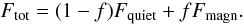 (3)To investigate detectability, we chose two different strategies. First, models with a single homogeneous atmosphere were considered, so called one-component (OC) models, where only the product Bf was determined. Second, two-component (TC) models were used, where B and f are naturally segregated, since f defines the relative surface fractions covered by the respective components, cf. Eq. (3). A further refinement of this model takes into account the generally different temperature stratifications of magnetic and non-magnetic regions. This temperature difference is well-known from the Sun (see, e.g., Solanki 1993, for an overview). This dichotomy in fitting strategies is addressed in the following and results are presented in separate subsections.
For both strategies adopted, we allow all fit parameters aside from Bf (OC) or B and f (TC) to vary freely in the fit (see last paragraph of Sect. 3.1). However, as explained above, log g was frequently used at a fixed literature value. Thus, we calculate χ2, cf. Eq. (2), for a range of values of Bf that we keep fixed in each inversion. In this way, we aim to avoid degeneracies that prevent the non-linear least-squares algorithm from finding the global minimum. This strategy implies that we do not aim to determine the other model parameters accurately. Our goal is to investigate whether introduction of magnetic flux (and how much) in the atmospheric model yields significantly better results.
To quantify our results, we determine the overall best-fit solution, i.e. where χ2 reaches its global minimum, as well as formal errors on Bf following Press et al. (1999). The formal 1σ range is adopted as our standard error. To claim detection of magnetic fields, we require the non-magnetic best-fit solution to lie outside the 3σ confidence level (CL). Non-detections are characterized by 3σ upper limits.
The CLs on χ2 are of a formal nature, since they depend on  , cf. Sect. 2.2. Errors deduced from these CLs would therefore represent the true errors only in the case of a “perfect” fit. In addition, the choice of a specific (Kurucz) input atmosphere introduces a bias that affects χ2 and thereby influences the formal error determination on Bf. However, spectral lines differ in their respective sensitivities to magnetic fields (usually expressed by their effective Landé factor, cf. Table 1). We employ both Zeeman sensitive and insensitive lines in simultaneous inversions. Each line’s different reaction to a certain postulated magnetic flux directly impacts the obtained best-fit χ2 for this Bf value. Therefore, provided the inversions are not dominated by systematic effects (see, however, Sect. 4.2.1), the CLs do allow us to evaluate whether evidence for a magnetic field is found, despite the above statements about their mostly formal nature. The CLs further provide an order-of-magnitude estimate on the uncertainty involved in the measurement.
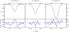 |
Fig. 2 Sun, line set A3, one-component model: Data and best-fits with Bf = 0 G (solid blue) and Bf = 225 G (dash-dotted red). |
3.2.1. One-component inversions
In the OC approach, we scan the dependence of χ2 on the single parameter Bf. This is done by performing inversions for a set of fixed Bf values. Best-fit solutions for χ2 and model parameters are obtained from each inversion.
In OC inversions we formally set f = 1 and investigate the line shaping effect due to the product Bf. Therefore, we assume a mean magnetic field covering the entire surface, aiming to avoid the degeneracy between B and f. The spacing of the Bf grid is usually 50 G, and is refined to 25 G close to the overall best-fit for better sampling of χ2 in this region.
3.2.2. Two-component inversions
Following the solar paradigm, magnetic fields in cool stars are expected to be concentrated in distinct elements that are usually described as flux tubes (Stenflo 1973; Spruit 1976; Solanki 1993). Our two-component (TC) inversions aim to take into account this physical fact by composing the atmospheric model of a magnetic and a field-free component. Thereby, we can investigate the impact of the f = 1 assumption made for OC models as well as the effect of a bimodal surface temperature distribution.
Hence, we perform three cases of TC inversions: those where both components have identical temperature, as well as those where magnetic regions are either cool, or warm with respect to the non-magnetic component. The equal temperature case was frequently used in the literature and allows for a more direct comparison of our results than OC inversions. Our incremental approach of increasing model complexity aims to distinguish between geometrical and temperature-related effects.
We compute the best-fit χ2 for each point of the B-f-plane defined by a grid of fixed B and f values. As a result, this approach is computationally much more expensive.
In the TC inversions, the model contains surface filling factor, f, as an additional fixed parameter, since we scan the B-f-plane. In addition to f, we introduce the additional fit parameter T2 for temperature at unit optical depth for the second component. For the equal temperature case, T2 and T1 are fitted, but kept equal. Both parameters can vary freely and independently in the cool and warm cases. To quantify our results, we construct formal CLs on the two-dimensional χ2-maps in analogy to the OC inversions.
In this paper, we perform TC inversions for the Sun and 59 Vir. For 59 Vir, for which a magnetic field is detected with a high CL, we investigate and compare the three different TC cases discussed above.
4. Results
We present our results in two kinds of figures, namely line fit plots and χ2-plots or -maps. Figure 2 is an example of line fit plots that help to assess the qualitative difference between magnetic and non-magnetic best-fit models. The upper panels contain the measured line profiles as ticks of length σi overplotted by best-fit solutions. Solid blue represents the overall best-fit solution, and dash-dotted red lines are used to draw either the non-magnetic, i.e. 0 G (if evidence for magnetic fields is found), or formal 3σ upper limit on Bf. Residuals are drawn in histogram style in the lower panels using the identical color and line style theme and visualize the difference between measured and calculated line profiles, scaled by factor 100. The purple error bar at the right end in each of the residual panels indicates σi.
The residuals contain smooth solid green lines that indicate the difference in line shape between the overall best-fit and the other best-fit model plotted, i.e. the change in line shape due to introduction of magnetic flux. The other fit parameters such as vsini, etc., adapt to each fixed Bf value, since they are allowed to vary freely. Hence, the green line does not represent the Zeeman pattern alone. It illustrates the combined effect due to ZB and different best-fit parameters for the two cases plotted.
Our inversions converged after relatively few iterations and although a given choice of starting values for the fit parameters (especially temperature) introduces a bias (if the χ2 surface has multiple minima), no dependence on these was found for the best-fit parameters.
Objects investigated sorted by increasing HD number.
Table 3 lists our results for Bf and overall best-fit parameters, i.e. those at , for both OC and TC inversions. The overall best-fit values for B and f from TC inversions are found in the text in the respective subsections. Columns 1–3 contain the star’s name, HD number and spectral type. Spanning these columns, we indicate if and for what kind of TC model results were obtained. The line sets used, as introduced in Table 1, are listed in Col. 4. Columns 5–7 list the overall best-fit , number of degrees of freedom (NDOF), and continuum signal-to-noise (S/N) measured in the data. Columns 8–10 provide literature values for effective temperature, Teff, as well as overall best-fit temperature at unit optical depth computed for continuum opacity at 5000 Å, T1, and, in the case of TC inversions, T2, in Kelvin, cf. Sect. 3.2. Column 11 contains literature values for logarithmic gravitational acceleration in cgs units, unless marked by an asterisk (*). In this case, log g was used as a free fit parameter, constrained by the pressure-sensitive Ca I line, and the overall best-fit value is presented. Columns 12–14 list the overall best-fit parameters obtained for macroturbulence, vmac, microturbulence, vmic, and projected rotational velocity, vsini, each in km s-1. Column 15 contains literature values for Bf, where available. Column 16 lists our results for average magnetic field with formal 1σ errors obtained from interpolation of the χ2-plots or -maps. The last Column 17 quotes the 3σ range of Bf rounded to 50 G.
Additional figures for OC results obtained can be found in the appendix. These include behavior of best-fit parameters with Bf as well as line profile plots for all OC results listed in Table 3 that are not included in the main article body.
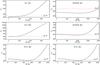 |
Fig. 3 χ2-plots obtained from one-component inversions. Object names are given inside the respective panels, and line sets used are mentioned in parentheses. 3σ confidence level on Bf indicated by dashed red horizontal lines. |
4.1. One-component inversions
OC inversions were carried out for 4 stars in different line sets, see Table 1. Figure 3 shows the χ2-plots determined for (from top left to bottom right) the Sun (A3), HD 68456 (A3), 61 Vir (B3), HD 68456 (B4), 59 Vir (B3), and 59 Vir (B4), where brackets indicate line sets used. The dashed red horizontal lines indicate the formal 3σ CL defined by  , cf. Sect. 3.2.1.
4.1.1. The Sun
The spectrum of sunlight reflected from Ganymede’s surface is the highest-quality spectrum used in this work with S/N ~ 700. We adopted solar abundances as determined by Grevesse & Sauval (1998) and Kurucz (1992) input atmosphere asun.dat13. Surface gravity was fixed at log g = 4.44.
The upper left panel of Fig. 3 clearly shows that the non-magnetic model yields our overall best-fit result for the Sun. We determine Bf = 0 + 90 G and a formal 3σ upper limit: Bf ≤ 200 G. χ2 increases smoothly and steeply above 200 G, indicating a robust non-detection. The overall best-fit parameters are listed in Table 3 and are consistent with the literature values published by V&F05: vsini = 1.63 km s-1, vmac = 3.98 km s-1, vmic = 0.85 km s-1.
Figure 2 shows the measured line profiles (black tick marks) of line set A3 overplotted by non-magnetic (blue) and magnetic (red, Bf = 225 G) best-fit calculated profiles. The agreement between either model and the measured line profiles is so close that amplified residuals have to be considered to view the difference. The most Zeeman-sensitive line, Cr I with geff = 2.00 (center), exhibits the strongest reaction to magnetic flux. This is indicated by the smooth green line. However, the amplitude of this reaction is of the same order of magnitude as σi.
A clear systematic signature is seen in the residuals, notably in the 5778.46 Å Fe I line. This W-shaped signature is not removed by ZB in this OC inversion and is roughly twice as large as the solid green line that indicates the difference between the non-magnetic and magnetic models. This indicates a systematic shortcoming in our ability to reproduce line shape and may indicate that, for instance, our approximate treatment of convection (as a macroturbulence) may be inadequate at this level of precision.
From this analysis, which is consistent with the upper limit of 140 G set by Stenflo & Lindegren (1977), also using broadening of intensity profiles, we can neither confirm nor rule out the result by Trujillo Bueno et al. (2004) of Bf ~ 130 G, since this value is consistent with our formal 3σ CL. The same is true for other, generally smaller, literature values of average (turbulent) magnetic fields determined for the quiet Sun (Solanki 2009). We conclude that magnetism averaged over the solar surface is too weak to be detected using this line set and method. Note that the above literature values refer to the quiet Sun, whereas the Sun was rather active at the time the analyzed data were recorded (13 October 2000). However, adding the active-region magnetic flux would raise the Bf value by a couple of 10 G only and thus would not affect our conclusions.
4.1.2. 61 Vir – HD 115617
The spectrum of the G6V field dwarf 61 Vir in data set B was an ideal candidate for a robust magnetic field measurement due to its slow rotation (R&S03: vsini < 2.2 km s-1), close-to solar metallicity ([Fe/H] = 0.05), Teff = 5571 K (latter two in V&F05), and low X-ray activity (NEXXUS2 database (Schmitt & Liefke 2004): log LX = 26.65). We used an input atmosphere calculated for Teff = 5500 K. log g = 4.47 (V&F05) was used as a fixed parameter.
The χ2-plot in the center left panel of Fig. 3 confirms the robust non-detection for 61 Vir. This is in agreement with expectations motivated by findings that link X-ray luminosity with magnetic flux (Pevtsov et al. 2003). The overall best-fit is reached for Bf = 0 G and formal 1σ and 3σ upper limits are established at Bf = 80 and 150 G, respectively. See Table 3 for details on other best-fit parameters. The lower 3σ upper limit obtained for 61 Vir than for the Sun can be explained by the higher Zeeman sensitivity of the line set B3 (61 Vir) relative to A3 (Sun).
We found one previous measurement of magnetic flux for 61 Vir in the literature. Gray (1984) determined  G ± 10%, where A0 is related to f by average viewing angle. This result is inconsistent with our null detection. We speculate that the difference between the two measurements is due to our higher data quality and different, possibly more sophisticated analysis technique.
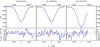 |
Fig. 4 59 Vir, line set B3, one-component model: data and best-fit with Bf = 500 G (solid blue) and Bf = 0 G (dash-dotted red). |
4.1.3. 59 Vir – HD 115383
59 Vir is a G0V field dwarf known for its activity and has been extensively studied by many authors. V&F05 measured its vsini = 7.4 km s-1, Teff = 6234 K, log g = 4.60 and [ Fe/H ] = 0.28 (relative to solar). log LX = 29.41 (NEXXUS2), approximately 2.8 dex higher than that of 61 Vir. Given its spectral type and observed rotation period Prot = 3.3 d measured by Donahue et al. (1996), 59 Vir would be classified as a young star. However, using multiple age-indicators, Lachaume et al. (1999) favor an age of 3.8 Gyr. Thus, 59 Vir is an interesting object to study regarding the age-activity relationship.
Inversions for 59 Vir were performed using line sets B3 and B4, cf. Table 1. In the latter case, surface gravity was well-constrained, despite the less-than-ideal fit to the Ca I line, and log g = 4.49 was obtained, consistent with the literature value. The other best-fit parameters are also consistent with the literature (Takeda et al. 2005; Sousa et al. 2008).
We determine  G for 59 Vir from line set B3 and
  G from B4, cf. the bottom left and right panels in Fig. 3. The 3σ CLs determined from both data sets are roughly the same with approximately 300 ≤ Bf ≤ 650 G. χ2 varies smoothly over the entire Bf range, and a steep incline is seen above Bf ~ 800 G. Furthermore, the best-fit solution for Bf = 0 G lies nearly 5σ from .
The 6173 Å line was assigned a slightly higher statistical weight, since it is the most Zeeman-sensitive line in the set with geff = 2.5. The blue wing of this line contains a blend due to Eu II that was not fully reproduced, despite our effort to include all available atomic line information in the inversions. Due to the presence of unidentified blends, the red wing had to be severed before reaching continuum. Line blends as well as the systematic signature seen also in the results for the Sun are clearly visible.
The residuals in Fig. 4 indicate improvement in fit quality due to introduction of magnetic flux for all lines. However, the largest differences between the magnetic (Bf = 500 G) and non-magnetic best-fit results are of the same magnitude as the S/N of the data. This result thus illustrates how difficult it is to detect ZB in optical Stokes I, even for relatively high values of Bf. The presence of systematic residual signatures similar to those found for the Sun and 61 Vir underline the need for rigorous and accurate implementation of radiative transfer and line broadening functions.
4.1.4. HD 68456
The F6 dwarf HD 68456 was of particular interest in our analysis, since data were available in both data sets and thus allowed our results to be tested for consistency. Since the dates of observation were nearly 4 years apart, we did not simultaneously invert lines from both sets. After all, changes in atmospheric parameters, for instance due to activity cycles, within this time span cannot be excluded. Fundamental parameters of this object are given by Hauck & Mermilliod (1998) (Teff = 6396 K, log g = 4.14, [Fe/H] = −0.29) and R&S03 (vsini = 9.8 km s-1). NEXXUS2 indicates a high level of activity of this star (log LX = 29.05). Furthermore, HD 68456 is a particularly interesting object to study in this context, since we are not aware of any previous ZB measurement in a late F-type star1.
Relatively fast rotation and high effective temperature combine to produce very shallow absorption lines in this star’s spectra. This fact complicated the analysis of line set A3 where lines are generally shallower than in data set B. Furthermore, data set A for this star was of lower quality than the other spectra analyzed in this work, containing individual data points that deviate significantly from the general line shape, while continuum S/N was approximately 400 in both data sets. The deviations seen are not consistent with the signature expected from a starspot.
The top and center right panels in Fig. 3 show our results obtained for line sets A3 and B4, respectively. For line set A3, the overall best-fit Bf = 1100 G, but no detection can be claimed. This is underlined by an F-test probability Pf = 0.21 for this result indicating spurious fit improvement. Using line set B4, however, we do find evidence for a magnetic field and obtain Bf ~ 1 kG, with the formal 3σ CL being 600 ≤ Bf ≤ 1200 G.
4.2. Two-component inversions
The concept of two-component (TC) inversions was introduced in Sect. 3.2.2. We carried out these more complex inversions for the Sun and 59 Vir. For the Sun, for which no one-component detection of a magnetic field was made, we did not expect reliable 2-component results. These inversions were carried out purely as a test. In the illustrative case discussed in the first subsection below we made the starting assumption for magnetic flux to be concentrated in cool regions, such as spots. The results are quite instructive regarding systematic effects. For 59 Vir, where the probability of attaining additional information from a two-component inversion is higher, we investigated the three cases mentioned above: equal temperatures for both components; warm magnetic component (warm case); cool magnetic component (cool case).
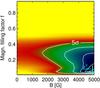 |
Fig. 5 χ2-map for the Sun, line set A3, TC model with cool magnetic regions. |
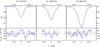 |
Fig. 6 Sun, line set A3, comparison of overall best-fit TC (B = 4900 G, f = 0.05, blue solid) and OC (Bf = 0 G, red dash-dotted) results. |
4.2.1. The Sun
Figure 5 shows the χ2-map calculated from TC inversions of solar line set A3. The input atmospheres used were asun.dat13 (cf. Sect. 4.1.1) for the warm and a Teff = 4750 K Kurucz atmosphere for the cool component. We obtain  , a value considerably lower than that obtained for the OC model, for B = 4950 G and f = 0.05. The Bf grid was calculated for field strengths of up to 5000 G, with filling factors up to 0.95 for B ≤ 2000 G and f ≤ 0.5 for B > 2000 G. The CLs are 235 ≤ Bf ≤ 250G(1σ) and 150 ≤ Bf ≤ 1400G(3σ), and thus would suggest evidence for very strong surface fields in the Sun. However, there are a number of problems with these results. For instance, magnetic fields in sunspots do not usually exceed ~3 kG while the average field strength of sunspots is roughly 1000−1300 G (Solanki & Schmidt 1993) and the field strength averaged over sunspot umbrae usually does not exceed 2500 G. In contrast, our 3σ confidence level suggests that B is well above 4 kG with f between 1– ~30% in disagreement with the observed sunspot coverage which is (always) below 1%. Furthermore, a multitude of measurements places the average Bf of the (quiet) Sun considerably lower (Solanki 2009). Last, the 3σ range for Bf is vastly larger than that found for the OC result. Therefore, we conclude that our fit was not well-constrained and that in this case the more complex TC model yielded less significant results than the simpler OC model.
Figure 6 helps to understand what happened here. The greatest decrease in χ2 was achieved by decreasing the systematic signature in the 5778 Å Fe I line. This apparent improvement in fit quality has stronger influence on χ2 than the deteriorating agreement between the measured and calculated profiles of the Cr I line at 5783 Å, since the former line contributes more degrees of freedom. Therefore, the magnetic field (or rather the lower temperature associated with the magnetic component) improves the fit of the Zeeman-insensitive (geff = 1.2) line, while the Zeeman-sensitive (geff = 2.0) line is less well matched. The worse fit in the blue Cr line wing is compensated in part by a small unidentified blend in the red wing that is falsely removed by the magnetic model. Thus, our conclusion is that this TC inversion is driven by systematic difficulties and yields a result that is less representative of the physical processes, albeit superior in terms of pure χ2. It therefore serves as an example of how line blends and other systematic effects on line shape affect our results.
4.2.2. 59 Vir – HD 115383
The results obtained for 59 Vir using OC models indicated formal 3σ detections of significant magnetic flux. To assess, if this detection is actually robust and significant, we performed TC inversions for this strongest candidate. The following results were obtained from our physically motivated TC inversions that distinguish between magnetic and non-magnetic components.
We investigated three different cases of TC inversions: equal temperatures, cool magnetic, and warm magnetic components. Thus, in the latter two cases, we investigate the effect of having different temperatures for the two components.
For the equal temperature case, we used the Teff = 6250 K Kurucz atmosphere for both components and coupled the two parameters T1 and T2, forcing them to be equal. In the cool case, we used tabulated atmospheres calculated for Teff = 6250 K and 5000 K for the non-magnetic and the magnetic component, respectively. The warm case was motivated by the warmer plage or network regions on the Sun. The Kurucz atmospheres were those with Teff = 6250 K for the magnetic and Teff = 6000 K for the non-magnetic regions. The temperature parameters T1 and T2 could vary freely and independently in both the warm and cool cases. The fitting ranges for T1 and T2 were large enough to allow turning the cool component into the hotter one and vice versa. The starting values of the fit parameters were identical in both cases, apart from the inverted values of T1 and T2 (the second temperature component was magnetic). All other starting values were identical to the OC inversions of 59 Vir.
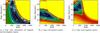 |
Fig. 7 Results obtained from TC inversions of 59 Vir, line set B3. |
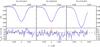 |
Fig. 8 59 Vir, line set B3: Comparing Bf = 120 G TC (blue solid) to Bf = 500 G OC (red dash-dotted) best-fit results. |
Equal temperatures:
Figure 7a shows the χ2-map obtained from our inversions of a model with equal temperatures for both components. As can be seen in Table 3, our overall best-fit parameters are virtually identical with our OC results. Even the two Bf values lie within their 1σ CLs.  is reached for B = 700 G and f = 0.6. However, even the 1σ CL spans a large range in f-values, and the 3σ CL is consistent with almost any f value. The reason for this lies in the χ2 surface, which has the well-known banana-shape, with a minimum running from the combination of high f and small B to the opposite extreme of small f and large B, while maintaining roughly equal magnetic flux (i.e. Bf). This is the signature of degeneracy between these two parameters. Of particular importance is the fact that in spite of the additional parameter f, the is identical to the OC case, which also indicates that there is not sufficient information in the data to distinguish between B and f. Furthermore, the formal Bf error margins for this case are larger than for the OC inversions and the other best-fit parameters nearly identical. Therefore, we conclude that a distinction made between magnetic and non-magnetic regions is insignificant.
Linsky et al. (1994, hereafter Li94) determined Bf = 190 G for 59 Vir (number published in Saar 1996) using an equal temperature TC model. Their Bf value is lower than, yet consistent with, our 3σBf range obtained from the TC inversions in the equal temperature case. It is, however, inconsistent with our 3σBf range determined from the OC inversions that favor higher Bf. At present it is not possible to say whether the difference to our results is due to differences in technique or due to the evolution of the stellar magnetic field.
Cool magnetic regions:
As in the above example for the Sun, we assume the majority of the magnetic flux to originate in starspots, i.e. in cool regions on the stellar surface. Figure 7b shows the χ2-map corresponding to this case. The overall best-fit  is reached for B = 250−300 G with f = 0.475 for both, i.e. Bf = 120−140 G. is lowered by 46.3 relative to the OC and TC equal temperature models and the formal 3σ confidence level is 0 ≤ Bf ≤ 320 G. The formal 3σ range in Bf is smaller than in the equal temperature TC case. The improvement in fit quality over the OC model is most clearly seen in the better matching central depth of the Zeeman-insensitive 6151 Å and of the Eu II blend to the Zeeman-sensitive line at 6173 Å, cf. Fig. 8. Both improvements are likely due to changes in level populations. The presence of a cool component enables a better matched line depth of Fe I, whereas the warm component contributes additional ionized europium thereby better matching the Eu II blend. In fact, the other two iron lines are also better matched by the TC inversion.
Figure 9 clearly shows that the difference in best-fit T1 and T2 within the 3σ CL lies between 1400−1600 K. This is roughly in agreement with the difference in temperatures chosen for the input atmospheres and the temperature differences between the quiet solar photosphere and sunspot umbrae.
Warm magnetic regions:
For this case, we employed a model containing slightly warmer magnetic than non-magnetic regions, i.e. assumed a model representative of plage or network-regions. This case is particularly interesting, since a warm second component contributes more flux than a cool one. Thus, the effect due to a certain Bf on line shape can be expected to be stronger.
Figure 7c illustrates our results.  is slightly higher than in the above cool case and yields B = 450 G and f = 0.6. Bf ranges from 210−325 G in the formal 1σ interval, while we find it consistent with 0−450 G at 3σ.
The 3σ range in B values is roughly the same as in the cool case, whereas the 5σ level is limited to lower B values. Opposite to the cool case, high-f solutions are favored. Thus, both cases favor a slight majority of the surface covered by warm elements. Despite the small (250 K) difference in Teff of the input atmospheres, the difference in best-fit parameters T2 and T1 within the 3σ CL ranges 1300−1400 K (ΔT = T2 − T1 in the warm case, since T2 > T1). This temperature difference is very similar to that found in the case of cool magnetic regions (for the 3σ CL).
Comparison of TC cases (equal, cool and warm):
The equal temperature TC case yields results in agreement with OC inversions, but wider CLs on Bf. Significantly lower is found in the two different temperature cases, also for the non-magnetic best-fit solutions (lowest χ2 for Bf = 0 G in equal, cool & warm cases: 287, 217, 231). Interestingly, the warm and cool TC cases tend towards virtually identical atmospheric configurations with nearly the same overall best-fit parameters for T1, T2 (though T1 and T2 are switched among the cool and warm cases), vsini, vmac, and vmic, cf. Table 3.
This suggests that the true reason for the improved fit to the observations is the presence of two temperature components. These simulate the inhomogeneity of the stellar atmosphere produced by starspots, granulation, oscillations, etc. and possibly also non-LTE effects in the line formation, which are not taken into account in the LTE modeling we have carried out.
A key difference between the different TC cases is the flux contribution from the respective magnetic component. Due to this difference in contrast, different Bf values may be expected. Our inversions yield comparable Bf for the OC and TC equal temperature model, while Bf is lower for the cases with different temperatures. Among these latter two, the warm case (brighter magnetic component) yields a slightly larger Bf. However, both are consistent with no magnetic field at the 3σ CL (though the warm case is not consistent with Bf = 0 G at 2σ).
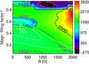 |
Fig. 9 ΔT-map for 59 Vir, cool case. Difference in K between T1 and T2 indicated by colors indicated in legend on right. Contours drawn for ΔT = T1 − T2 = 0 K (orange), 500 K (magenta), 1400 K (blue), 1600 K (purple), and 2000 K (black). White contours indicate 3 and 5σ CLs. The large white plus indicates the point of overall best fit. |
5. Discussion
To assess detectability of ZB for this kind of analysis, we first discuss the general uncertainties and sources of error before examining the impact of model assumptions.
Our analysis is prone to uncertainties from various sources, such as degeneracies among various line broadening agents and uncertainties in information used as input (atmospheres, line data, lines used, etc.). We attempted to avoid degeneracy among line broadening agents by allowing all fit parameters to vary freely for given average magnetic fields. This approach helped to nudge the non-linear χ2-minimization routine towards the global minimum. In addition, it provided a clear visualization (see Fig. 3) of the range of acceptable Bf values, thereby providing very solid upper limits on Bf of, say, a few hundred to 1.5 kG depending on the star.
More spectral lines could have provided more stringent constraints on model parameters. Unfortunately, our choice of lines was severely limited by the small wavelength coverage of the CES spectra. Temperature stratification would have been even better constrained by using lines from multiple ionization stages. In order to achieve the fit quality presented in this paper, however, we relied on lines from different excitation potentials. We had found that some combinations of lines yielded better fit agreement than others. The reasons for this empirical fact are likely related to blends; specifically, to blend abundances (often unconstrained), lack of literature on transition parameters needed for SPINOR, uncertainties in oscillator strengths or rest-wavelengths, and unidentified line blends or even relative displacements of blend wavelengths due to convection. For a literature comparison of the fit quality presented here, see Frutiger et al. (2005) who applied SPINOR in simultaneous inversions of 14 lines for α Cen A and B, including lines from different ionization stages. Their Figs. 2 and 3 clearly illustrate the larger discrepancy between model and data when a large number of lines is used.
Small systematic effects (best visible in the spectral difference between observed and computed lines profiles) complicated our analysis. The high quality of the data revealed these systematic shortcomings in reproducing real line profiles. The data for the Sun was both the highest quality spectrum (in terms of S/N) and one of the least rotationally broadened. The fact that the TC inversions for the Sun produced such implausible results may indicate that a limit was surpassed for an adequate representation of line profiles by simple broadening functions such as the radial-tangential macroturbulence profile. However, some of the difficulties in the solar TC inversion were also related to the lower Zeeman sensitivity of line set A3, in addition to the low level of solar magnetism and the data-related problems of line blends, etc. Further candidates for the origin of the systematic signatures at this level may be related to any of a number of sources, such as the implementation of limb-darkening and disk-integration, temperature stratification, neglect of stellar convection (granulation) and oscillations, differential rotation, neglect of non-LTE effects, depth-dependent magnetic field strength, scattered light in CES data, etc. In addition, the temperature gradients of active stars may differ significantly from those of inactive stars. Thus, the representation of magnetic regions by “quiet” atmospheres may also be too crude an approximation, since it neglects inhibition of convection and the influence of magnetic fields on temperature stratification. Thus, applicability of LTE Kurucz input atmospheres could be questioned. Non-LTE effects might also be seen, since the systematic residual signature appears to be enhanced in hotter stars. The analysis thus suffers from a multitude of highly degenerate effects originating in approximations. Most of these flaws cannot be easily resolved, however, and there are valid reasons for adopting at least some of these approximations.
Two kinds of fitting strategies were explored: one-component (OC) and two-component (TC) models, cf. Sect. 3.2 for details. OC models assume a homogeneous atmosphere with a single temperature stratification and an average magnetic field, Bf, covering the entire stellar surface. For the Sun and 61 Vir, both stars with low X-ray activity, our OC results excluded Bf exceeding a few hundred Gauss. OC inversions further yielded evidence of 500 G to 1 kG fields for two faster rotators with higher X-ray luminosity, namely 59 Vir and HD 68456. As could be expected from its larger maximum geff value and geff coverage, line set B3 was more sensitive to ZB than A3.
Two-component (TC, cf. Sect. 3.2.2) inversions were performed to distinguish between magnetic and non-magnetic surface regions. For our solar spectrum in line set A3, we present a case study that assumed the magnetic fields to be concentrated in spots, i.e. in significantly cooler regions. However, the solar TC model was driven by systematic effects (partly due to weak blends in the line wings) and yielded a result inconsistent with the OC result and the literature.
For 59 Vir, we explored three different cases of TC inversions: a) equal temperatures for both components; b) a cool magnetic; and c) a warm magnetic component. We find that the equal temperature TC case is consistent with the results from the OC inversions. Furthermore, the Bf determined is consistent with the only available literature value. However, no improvement in χ2 is seen over the OC model, while an additional fit parameter, f, was introduced. This is consistent with the well known result that the product Bf is much better constrained than B and f individually (Saar 1990a).
The picture changes, however, when the model takes into account two different temperatures in the two components, as was done for the cool (spots) and warm (plage and network regions) TC cases. In fact, a significant improvement of χ2 was seen for both of these more complex inversions. Independent of the input atmospheres used for the two components, these inversions converged towards a very similar photospheric model featuring similar coverage (f ≈ 50%) by hot and cool features with ΔT ≈ 1300 K. The difference in  between the warm and cool case is probably the result of the a priori choice of input atmospheres. Magnetic flux did not play a deciding role in the inversions’ ability to converge towards this common overall best-fit model. Note, however, that the improvement of the fit comes at the expense of additional free parameters (2 new parameters are introduced compared to the OC case).
For both the warm and the cool TC case, Bf was lower than in the OC or TC equal temperature case and consistent with no magnetic field at the 3σ CL (however, not at 2σ in the warm case). Thus, while some evidence for ZB was found in these cases, no detection can be claimed when allowing for two different temperature components, one magnetic, the other field free.
Given the significant improvement of , we find that model assumptions impact our ability to reproduce the observed line shape more strongly than the presence or absence of ZB in optical Stokes I, even for relatively high Landé factors. At the same time, the presence of ZB is not excluded, either.
As a next step, even more complex models might be invoked. However, this does not appear to be expedient at this point, given the limited number of lines used for analysis, the approximative treatment of line profiles (e.g. the radial-tangential macroturbulence and the height-independent microturbulence), the smallness of the Zeeman signature, and the fact that the TC inversions of 59 Vir already reached the noise limit.
A more prudent approach would be to increase sensitivity to ZB. This could be done by using high-resolution infrared spectra. In this way, the λ2 dependence of Eq. (1) could be exploited to provide stringent constraints that are in addition to the differential Bf-response that was at the base for this investigation. Furthermore, the IR contrast between cool and warm regions would be lower, thereby enhancing Zeeman signatures (e.g. Johns-Krull 2007). In M-dwarfs, successful measurements of strong magnetic fields have been reported using molecular lines, e.g. using FeH lines in the Wing-Ford bands (Reiners & Basri 2006, 2007). With the majority of their flux in the infrared and strong fields, these stars constitute prime candidates for direct Bf measurements using spectral line inversion as outlined in this work.
6. Summary
In this paper, we investigated detectability of ZB in optical Stokes I spectra of the Sun and three slowly rotating sun-like stars by performing spectral line inversion with SPINOR.
Thanks to the ability of SPINOR to perform spectral line inversion, different scenarios could be compared and model assumptions evaluated by scanning the χ2 plane for fixed Bf, or combinations of B and f, values. This approach enabled us to investigate the form of χ2 as a function of Bf as shown in Fig. 3 and therefrom determine formal errors on Bf.
Systematic uncertainties in our analysis are in part related to literature used as input, such as atomic line data and elemental abundances. Due to the small magnitude of the Zeeman broadening even weak line blends complicated the analysis. Approximations, such as the representation of turbulence in the stellar atmosphere by radial-tangential macroturbulence and height-independent microturbulence, also influenced our results.
OC inversions excluded the presence of significant magnetic flux (Bf < 150 G at the 3σ CL) for the Sun and 61 Vir. Our results for HD 68456 may be interpreted as first evidence for a magnetic field in a late F-type dwarf obtained by the ZB technique, with Bf ≈ 1 kG and formal 3σ errors of approximately 350 G. The OC result for 59 Vir is  G.
G.
The TC equal temperature case yielded Bf = 420 G for 59 Vir, a higher value than that reported by Li94, but consistent within the (large) formal 1σ error. TC inversions with components of different temperatures were consistent with Bf between 0 G and 450 G at the 3σ CL. The case of a warm magnetic component was inconsistent with an absence of magnetic field at 2σ. Previous investigations of this kind frequently used models similar to our equal temperature TC case. Our investigation of the different TC inversion cases demonstrates the strong influence of model assumptions. In fact, the freedom to freely and independently vary both atmospheric temperatures in TC models was shown to influence line shape more strongly than ZB for the lines used in this work, cf. Sect. 4.2.2. The improvement of χ2 due to a second component of different temperature was significantly larger than that due to a magnetic field, irrespective of whether the magnetic component was defined as warm, or cool. The present data quality exceeds that of previous studies, while our sensitivity to Zeeman broadening as expressed by the geff values in our line sets is comparable to that in the literature with the exception of studies in the infrared.
We conclude that measurements of ZB in optical Stokes I data of slowly rotating sun-like stars are subject to large uncertainties. These are mostly due to data related uncertainties, assumptions on atmospheric models, approximations in line broadening agents, and degeneracy between line broadening agents. However, the Zeeman sensitivity of every individual line (as expressed by its geff value) differs from line to line by a factor of up to 2.5. This provides a powerful discriminant for our analysis, since the other relevant broadening effects depend mostly on temperature or wavelength and are thus essentially the same for all lines used. It is this differential reaction of each spectral line to a given magnetic field that ensured the significance of the measurements presented in this work, despite the small magnitude of the ZB signature.
The most promising way to improve the present approach is to further exploit the λ2-dependence of ZB and use longer wavelength data. In the (near) infrared, Zeeman broadening clearly dominates over Doppler effects and Zeeman splitting can be seen directly, see e.g. Saar (1994); Johns-Krull & Valenti (1996); Valenti & Johns-Krull (2001). New high-resolution near infrared spectrographs have become available for these tasks.
Online material
Appendix A: Online figures
We present additional figures illustrating our OC results in this appendix.
A.1. Additional one-component fit results
Figure A.1 shows the OC fit results not presented in the main article body whose corresponding χ2-plots were included in Fig. 3. The best-fit models drawn are mentioned in the respective captions of the sub-figures.
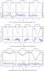 |
Fig. A.1 Additional comparison of overall best-fit results from one-component inversions with non-magnetic models and 3σ upper limits, respectively. |
A.2. Free fit parameters
Figure A.2 shows the behavior of the free fit parameters with Bf in the OC inversions. Red error bars indicate formal singular value decomposition (SVD) errors obtained from SPINOR. They also indicate the spacing of the Bf grid scanned, thereby illustrating the higher sampling close to  . Generally, fit parameters behave smoothly, apart from regions where small numerical jumps are visible, such as for vsini in Fig. A.2a. The center panel in each sub-figure labeled vturb contains both macro- and microturbulent velocities, with macroturbulence generally stronger than microturbulence. Degeneracy of fit parameters is evident from the combined reaction of the parameter set caused by the fixed values of Bf.
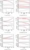 |
Fig. A.2 Behavior of best-fit parameters with Bf using one-component models. Plot organized the same way as Fig. 3. vturb indicates micro- and macroturbulent velocities, with macroturbulence usually larger than microturbulence. |
But note the work of Donati et al. (2008) on the changing magnetic field topology on τ Boo (F7 IV-V, Gray et al. 2001).
Acknowledgments
We thank the referee John D. Landstreet for his detailed report that resulted in a much clearer explanation of our analysis and a significantly better manuscript. Thanks are due to the following people: Christian Schröder for observing data set B; A. Lagg at MPS for SPINOR related support; S. H. Saar for very fruitful advice and discussion. R.I.A. and A.R. acknowledge research funding from the DFG under an Emmy Noether Fellowship (RE 1664/4-1). R.I.A. further acknowledges funding by the Fonds National Suisse de la Recherche Scientifique (FNRS). The work of S.K.S. has been partially supported by the WCU grant No. R31-10016 funded by the Korean Ministry of Education, Science and Technology. This research has made use of NASA’s Astrophysics Data System Bibliographic Services and the SIMBAD database, operated at CDS, Strasbourg, France.
References
- Anstee, S. D., & O’Mara, B. J. 1995, MNRAS, 276, 859 [NASA ADS] [CrossRef] [Google Scholar]
- Barklem, P. S., & O’Mara, B. J. 1997, MNRAS, 290, 102 [Google Scholar]
- Barklem, P. S., O’Mara, B. J., & Ross, J. E. 1998, MNRAS, 296, 1057 [Google Scholar]
- Basri, G., & Marcy, G. W. 1988, ApJ, 330, 274 [NASA ADS] [CrossRef] [Google Scholar]
- Beckers, J. M. 1969, A table of Zeeman Multiplets, AFCRL-69-0115, No. 371 [Google Scholar]
- Berdyugina, S. V. 2005, Liv. Rev. Sol. Phys., 2, 8 [Google Scholar]
- Cayrel de Strobel, G., Soubiran, C., Friel, E. D., Ralite, N., & Francois, P. 1997, A&AS, 124, 299 [NASA ADS] [CrossRef] [EDP Sciences] [Google Scholar]
- Donahue, R. A., Saar, S. H., & Baliunas, S. L. 1996, ApJ, 466, 384 [NASA ADS] [CrossRef] [Google Scholar]
- Donati, J. 2008, in 14th Cambridge Workshop on Cool Stars, Stellar Systems, and the Sun, ed. G. van Belle, ASP Conf. Ser., 384, 156 [NASA ADS] [Google Scholar]
- Donati, J., & Landstreet, J. D. 2009, ARA&A, 47, 333 [NASA ADS] [CrossRef] [MathSciNet] [Google Scholar]
- Donati, J., Moutou, C., Farès, R., et al. 2008, MNRAS, 385, 1179 [NASA ADS] [CrossRef] [Google Scholar]
- Favata, F., Reale, F., Micela, G., et al. 2000, A&A, 353, 987 [NASA ADS] [Google Scholar]
- Frutiger, C. 2000, Ph.D. Thesis, Institute of Astronomy, ETH Zürich [Google Scholar]
- Frutiger, C., Solanki, S. K., Fligge, M., & Bruls, J. H. M. J. 2000, A&A, 358, 1109 (Fru00) [NASA ADS] [Google Scholar]
- Frutiger, C., Solanki, S. K., & Mathys, G. 2005, A&A, 444, 549 (Fru05) [NASA ADS] [CrossRef] [EDP Sciences] [Google Scholar]
- Gray, D. F. 1975, ApJ, 202, 148 [NASA ADS] [CrossRef] [Google Scholar]
- Gray, D. F. 1984, ApJ, 277, 640 [NASA ADS] [CrossRef] [Google Scholar]
- Gray, D. F. 2008, The Observation and Analysis of Stellar Photospheres (Cambridge University Press) (Gr08) [Google Scholar]
- Gray, R. O., Napier, M. G., & Winkler, L. I. 2001, AJ, 121, 2148 [NASA ADS] [CrossRef] [Google Scholar]
- Grevesse, N., & Sauval, A. J. 1998, Space Sci. Rev., 85, 161 [NASA ADS] [CrossRef] [Google Scholar]
- Hall, J. C., & Lockwood, G. W. 2004, ApJ, 614, 942 [NASA ADS] [CrossRef] [Google Scholar]
- Hauck, B., & Mermilliod, M. 1998, A&AS, 129, 431 [NASA ADS] [CrossRef] [EDP Sciences] [Google Scholar]
- Johns-Krull, C. M. 2007, ApJ, 664, 975 [NASA ADS] [CrossRef] [Google Scholar]
- Johns-Krull, C. M., & Valenti, J. A. 1996, ApJ, 459, L95 [NASA ADS] [CrossRef] [Google Scholar]
- Johns-Krull, C. M., & Valenti, J. A. 2000, in Stellar Clusters and Associations: Convection, Rotation, and Dynamos, ed. R. Pallavicini, G. Micela, & S. Sciortino, ASP Conf. Ser., 198, 371 [Google Scholar]
- Kupka, F., Ryabchikova, T. A., Piskunov, N. E., Stempels, H. C., & Weiss, W. W. 2000, Vienna Atomic Line Database [Online], Baltic Astronomy, 9, 590, http://vald.astro.univie.ac.at [Google Scholar]
- Kurucz, R. L. 1992, in The Stellar Populations of Galaxies, ed. B. Barbuy, & A. Renzini, IAU Symp., 149, 225 [Google Scholar]
- Kurucz, R. L., & Bell, B. 1995, Atomic Line Data Kurucz CD-ROM No. 23, Smithsonian Astrophysical Observatory, http://cfa-www.harvard.edu/amp/ampdata/kurucz23/sekur.html [Google Scholar]
- Kurucz, R. L., Furenlid, I., Brault, J., & Testerman, L. 1984, National Solar Observatory Atlas No. 1 – Solar Flux Atlas From 296 to 1300 nm (University Publisher, Harvard University) [Google Scholar]
- Lachaume, R., Dominik, C., Lanz, T., & Habing, H. J. 1999, A&A, 348, 897 [NASA ADS] [Google Scholar]
- Linsky, J. L., Andrulis, C., Saar, S. H., Ayres, T. R., & Giampapa, M. S. 1994, in Cool Stars, Stellar Systems, and the Sun, ed. J.-P. Caillault, ASP Conf. Ser., 64, 438 [NASA ADS] [Google Scholar]
- Lites, B. W., Bida, T. A., Johannesson, A., & Scharmer, G. B. 1991, ApJ, 373, 683 [NASA ADS] [CrossRef] [Google Scholar]
- Maggio, A., Pallavicini, R., Reale, F., & Tagliaferri, G. 2000, A&A, 356, 627 [NASA ADS] [Google Scholar]
- Marcy, G. W. 1982, PASP, 94, 989 [NASA ADS] [CrossRef] [Google Scholar]
- Mathys, G. 1990, A&A, 232, 151 [NASA ADS] [Google Scholar]
- Mathys, G., Hubrig, S., Landstreet, J. D., Lanz, T., & Manfroid, J. 1997, A&AS, 123, 353 [Google Scholar]
- Pevtsov, A. A., Fisher, G. H., Acton, L. W., et al. 2003, ApJ, 598, 1387 [NASA ADS] [CrossRef] [Google Scholar]
- Pizzolato, N., Maggio, A., Micela, G., Sciortino, S., & Ventura, P. 2003, A&A, 397, 147 [NASA ADS] [CrossRef] [EDP Sciences] [Google Scholar]
- Press, W. H., Teukolsky, S. A., Vetterling, W. T., & Flannery, B. P. 1999, Numerical recipes in C., The art of scientific computing (Cambridge: University Press), 2nd edn. reprinted with corrections [Google Scholar]
- Preston, G. W. 1971, ApJ, 164, 309 [NASA ADS] [CrossRef] [Google Scholar]
- Reiners, A., & Basri, G. 2006, ApJ, 644, 497 [NASA ADS] [CrossRef] [Google Scholar]
- Reiners, A., & Basri, G. 2007, ApJ, 656, 1121 [NASA ADS] [CrossRef] [Google Scholar]
- Reiners, A., & Basri, G. 2009, A&A, 496, 787 [NASA ADS] [CrossRef] [EDP Sciences] [Google Scholar]
- Reiners, A., & Schmitt, J. H. M. M. 2003, A&A, 398, 647 (R&S03) [NASA ADS] [CrossRef] [EDP Sciences] [Google Scholar]
- Robinson, R. D., Worden, S. P., & Harvey, J. W. 1980, ApJ, 236, L155 [NASA ADS] [CrossRef] [Google Scholar]
- Robinson, Jr., R. D. 1980, ApJ, 239, 961 [NASA ADS] [CrossRef] [Google Scholar]
- Rüedi, I., Solanki, S. K., Mathys, G., & Saar, S. H. 1997, A&A, 318, 429 [NASA ADS] [Google Scholar]
- Saar, S. H. 1988, ApJ, 324, 441 [NASA ADS] [CrossRef] [Google Scholar]
- Saar, S. H. 1990a, in Solar Photosphere: Structure, Convection, and Magnetic Fields, ed. J. O. Stenflo, IAU Symp., 138, 427 [NASA ADS] [Google Scholar]
- Saar, S. H. 1990b, Mem. Soc. Astron. Ital., 61, 559 [NASA ADS] [Google Scholar]
- Saar, S. H. 1994, in Infrared Solar Physics, ed. D. M. Rabin, J. T. Jefferies, & C. Lindsey, IAU Symp., 154, 437 [Google Scholar]
- Saar, S. H. 1996, in Magnetodynamic Phenomena in the Solar Atmosphere – Prototypes of Stellar Magnetic Activity, ed. Y. Uchida, T. Kosugi, & H. S. Hudson, IAU Colloq., 153, 367 [Google Scholar]
- Schmitt, J. H. M. M. 2001, in Recent Insights into the Physics of the Sun and Heliosphere: Highlights from SOHO and Other Space Missions, ed. P. Brekke, B. Fleck, & J. B. Gurman, IAU Symp., 203, 475 [Google Scholar]
- Schmitt, J. H. M. M., & Liefke, C. 2004, A&A, 417, 651 [NASA ADS] [CrossRef] [EDP Sciences] [Google Scholar]
- Semel, M. 1989, A&A, 225, 456 [NASA ADS] [Google Scholar]
- Solanki, S. K. 1993, Space Sci. Rev., 63, 1 [NASA ADS] [CrossRef] [Google Scholar]
- Solanki, S. K. 2009, in ASP Conf. Ser., ed. S. V. Berdyugina, K. N. Nagendra, & R. Ramelli, 405, 135 [Google Scholar]
- Solanki, S. K., & Schmidt, H. U. 1993, A&A, 267, 287 [NASA ADS] [Google Scholar]
- Solanki, S. K., & Stenflo, J. O. 1985, A&A, 148, 123 [NASA ADS] [Google Scholar]
- Sousa, S. G., Santos, N. C., Mayor, M., et al. 2008, A&A, 487, 373 [NASA ADS] [CrossRef] [EDP Sciences] [MathSciNet] [Google Scholar]
- Spruit, H. C. 1976, Sol. Phys., 50, 269 [NASA ADS] [CrossRef] [Google Scholar]
- Stenflo, J. O. 1973, Sol. Phys., 32, 41 [NASA ADS] [CrossRef] [Google Scholar]
- Stenflo, J. O., & Lindegren, L. 1977, A&A, 59, 367 [NASA ADS] [Google Scholar]
- Takeda, Y., Ohkubo, M., Sato, B., Kambe, E., & Sadakane, K. 2005, PASJ, 57, 27 [NASA ADS] [CrossRef] [Google Scholar]
- Trujillo Bueno, J., Shchukina, N., & Asensio Ramos, A. 2004, Nature, 430, 326 [Google Scholar]
- Valenti, J. A., & Fischer, D. A. 2005, ApJS, 159, 141 (V&F05) [NASA ADS] [CrossRef] [MathSciNet] [Google Scholar]
- Valenti, J. A., & Johns-Krull, C. 2001, in Magnetic Fields Across the Hertzsprung-Russell Diagram, ed. G. Mathys, S. K. Solanki, & D. T. Wickramasinghe, ASP Conf. Ser., 248, 179 [Google Scholar]
- Wilson, P. R. 1994, Solar and stellar activity cycles, Cambridge Astrophysics Series (Cambridge, MA: Cambridge University Press) [Google Scholar]
- Wittmann, A. 1974, Sol. Phys., 35, 11 [NASA ADS] [CrossRef] [EDP Sciences] [Google Scholar]
All Tables
All Figures
|
Fig. 1 Sample CES spectra illustrating data quality. Continua are shifted by ±0.3 from unity for visibility. Blue dash-dotted vertical lines indicate spectral lines used for analysis. Upper panel: data set A. Upper black spectrum: sunlight reflected from Jupiter’s moon Ganymede; lower red spectrum: HD 68456 (F6V, vsini ≈ 10 km s-1). Lower panel: data set B. Upper black spectrum: inactive and slow rotator 61 Vir (G6V); lower red spectrum: active and faster rotator 59 Vir (G0V, vsini ≈ 6.5 km s-1). |
| In the text | |
|
Fig. 2 Sun, line set A3, one-component model: Data and best-fits with Bf = 0 G (solid blue) and Bf = 225 G (dash-dotted red). |
| In the text | |
|
Fig. 3 χ2-plots obtained from one-component inversions. Object names are given inside the respective panels, and line sets used are mentioned in parentheses. 3σ confidence level on Bf indicated by dashed red horizontal lines. |
| In the text | |
|
Fig. 4 59 Vir, line set B3, one-component model: data and best-fit with Bf = 500 G (solid blue) and Bf = 0 G (dash-dotted red). |
| In the text | |
|
Fig. 5 χ2-map for the Sun, line set A3, TC model with cool magnetic regions. |
| In the text | |
|
Fig. 6 Sun, line set A3, comparison of overall best-fit TC (B = 4900 G, f = 0.05, blue solid) and OC (Bf = 0 G, red dash-dotted) results. |
| In the text | |
|
Fig. 7 Results obtained from TC inversions of 59 Vir, line set B3. |
| In the text | |
|
Fig. 8 59 Vir, line set B3: Comparing Bf = 120 G TC (blue solid) to Bf = 500 G OC (red dash-dotted) best-fit results. |
| In the text | |
|
Fig. 9 ΔT-map for 59 Vir, cool case. Difference in K between T1 and T2 indicated by colors indicated in legend on right. Contours drawn for ΔT = T1 − T2 = 0 K (orange), 500 K (magenta), 1400 K (blue), 1600 K (purple), and 2000 K (black). White contours indicate 3 and 5σ CLs. The large white plus indicates the point of overall best fit. |
| In the text | |
|
Fig. A.1 Additional comparison of overall best-fit results from one-component inversions with non-magnetic models and 3σ upper limits, respectively. |
| In the text | |
|
Fig. A.2 Behavior of best-fit parameters with Bf using one-component models. Plot organized the same way as Fig. 3. vturb indicates micro- and macroturbulent velocities, with macroturbulence usually larger than microturbulence. |
| In the text | |
Current usage metrics show cumulative count of Article Views (full-text article views including HTML views, PDF and ePub downloads, according to the available data) and Abstracts Views on Vision4Press platform.
Data correspond to usage on the plateform after 2015. The current usage metrics is available 48-96 hours after online publication and is updated daily on week days.
Initial download of the metrics may take a while.