| Issue |
A&A
Volume 522, November 2010
|
|
|---|---|---|
| Article Number | A7 | |
| Number of page(s) | 28 | |
| Section | Extragalactic astronomy | |
| DOI | https://doi.org/10.1051/0004-6361/201014746 | |
| Published online | 26 October 2010 | |
PMAS optical integral field spectroscopy of luminous infrared galaxies
II. Spatially resolved stellar populations and excitation conditions*,,**
1
Departamento de Astrofísica Molecular e InfrarrojaInstituto de Estructura
de la Materia, CSIC, 28006
Madrid, Spain
e-mail: This email address is being protected from spambots. You need JavaScript enabled to view it.
2
I. Physikalisches Institut, Universität zu Köln,
50937
Köln,
Germany
3
European Organisation for Astronomical Research in the Southern
Hemisphere, Karl-Schwarzschild-Strasse 2, 85748
Garching bei München,
Germany
Received:
7
April
2010
Accepted:
1
June
2010
Abstract
Context. The general properties (e.g., activity class, star formation rates, metallicities, extinctions, average ages, etc.) of luminous (LIRGs) and ultraluminous infrared galaxies (ULIRGs) in the local universe are well known because large samples of these objects have been the subject of numerous spectroscopic works over the past three decades. There are, however, relatively few studies of the spatially-resolved spectroscopic properties of large samples of LIRGs and ULIRGs using integral field spectroscopy (IFS).
Aims. We are carrying out an IFS survey of local (z < 0.26) samples of LIRGs and ULIRGs to characterize their two-dimensional spectroscopic properties. The main goal of this paper is to study the spatially resolved properties of the stellar populations and the excitation conditions in a sample of LIRGs.
Methods. We analyze optical (3800–7200 Å) IFS data taken with the Potsdam Multi-Aperture Spectrophotometer (PMAS) of the central few kiloparsecs of eleven LIRGs. To study these stellar populations, we fit the optical stellar continuum and the hydrogen recombination lines of selected regions in the galaxies. We analyzed the excitation conditions of the gas using the spatially resolved properties of the brightest optical emission lines. We complemented the PMAS observations with existing HST/NICMOS near-infrared continuum and Paα imaging.
Results. The optical continua of selected regions in our LIRGs are well fitted with a combination of an evolved (~0.7−10 Gyr) stellar population with an ionizing stellar population (1−20 Myr). The latter population is more obscured than the evolved population, and has visual extinctions in good agreement with those obtained from the Balmer decrement. Except for NGC 7771, we find no clear that there is an important contribution to the optical light from an intermediate-aged stellar population (~100−500 Myr). Even after correcting for the presence of stellar absorption, a large number of spaxels with low observed equivalent widths of Hα in emission still show enhanced [N ii]λ6584/Hα and [S ii]λλ6717, 6731/Hα ratios. These ratios are likely to be produced by a combination of photoionization in H ii regions and diffuse emission. These regions of enhanced line ratios are generally coincident with low surface-brightness H ii regions and diffuse emission detected in the Hα and Paα images. We used the PMAS spatially resolved line ratios and the NICMOS Paα photometry of H ii regions to derive the fraction of diffuse emission in LIRGs. We find that this fraction varies from galaxy to galaxy, and it is generally less than 60%, as found in other starburst galaxies.
Key words: galaxies: evolution / galaxies: nuclei / galaxies: star formation / galaxies: structure / infrared: galaxies
Based on observations collected at the German-Spanish Astronomical Center, Calar Alto, jointly operated by the Max-Planck-Institut für Astronomie Heidelberg and the Instituto de Astrofísica de Andalucía (CSIC).
Figures 1b–1j and 2b–2j are only available in electronic form at http://www.aanda.org
© ESO, 2010
1. Introduction
Luminous and ultraluminous infrared galaxies (LIRGs and ULIRGs) with infrared 8−1000 μm luminosities LIR = 1011−1012 L⊙ and LIR = 1012−1013 L⊙, respectively (see Sanders & Mirabel 1996) are among the most luminous objects in the local universe, and are believed to be powered by strong star formation and/or AGN activity. The main properties of local LIRGs and ULIRGs are well known because these two classes of galaxies have been extensively studied using imaging and spectroscopy over the last three decades. These properties include, among others, morphologies (e.g., Veilleux et al. 2002; Sanders & Ishida 2004; Scoville et al. 2000; Bushouse et al. 2002; Alonso-Herrero et al. 2006), the nuclear activity class, star formation rates, and extinctions (e.g., Heckman et al. 1987, 2000; Armus et al. 1989; Kim et al. 1995, 1998; Veilleux et al. 1995, 1999; Goldader et al. 1995; Wu et al. 1998; Rigopoulou et al. 1999; Yuan et al. 2010), stellar populations (e.g., Poggianti & Wu 2000; Chen et al. 2009; Rodríguez Zaurín et al. 2009, 2010a), metallicities (e.g., Rupke et al. 2008), and molecular gas content (e.g., Sanders et al. 1991; Gao & Solomon 2004; Graciá-Carpio et al. 2006, 2008).
There are, however, relatively few studies of the spatially-resolved spectroscopic properties of LIRGs and ULIRGs using integral field spectroscopy (IFS). Most works have focused on individual famous objects or small samples (e.g., Colina et al. 1999; Arribas et al. 2001; Murphy et al. 2001; Lípari et al. 2004a,b; Colina et al. 2005; Monreal-Ibero et al. 2006; García-Marín et al. 2006; Reunanen, et al. 2007; Bedregal et al. 2009). IFS instruments working in the optical and infrared spectral ranges on 4 and 8 m-class telescopes are now ubiquitous, and thus this situation is changing rapidly. Our group is involved in an ambitious project intended to characterize the detailed optical and infrared spectroscopic properties of local samples of LIRGs and ULIRGs using a variety of IFS facilities.
This is the second paper in a series presenting observations with the Potsdam Multi-Aperture Spectrophotometer (PMAS, Roth et al. 2005) of the northern portion of a sample of local LIRGs defined by Alonso-Herrero et al. (2006). The PMAS sample is in turn part of the larger IFS survey of nearby (z < 0.26) LIRGs and ULIRGs in the northern and the southern hemispheres using different IFS instruments. The optical ones include, apart from the PMAS instrument, the VIMOS instrument (Le Fèvre et al. 2003) on the VLT, and the INTEGRAL+WYFFOS system (Arribas et al. 1998; Bingham et al. 1994) on the William Herschel Telescope (WHT). The first results of this project can be found in Alonso-Herrero et al. (2009, hereafter Paper I) for the PMAS atlas of LIRGs, García-Marín et al. (2009a,b) for the INTEGRAL results of ULIRGs, and Arribas et al. (2008), Monreal-Ibero et al. (2010a) and Rodríguez Zaurín et al. (2010b) for the VIMOS results. Additionally, Pereira-Santaella et al. (2010) studied the spatially resolved mid-infrared properties of LIRGs using the spectral mapping capability of IRS on Spitzer, and Bedregal et al. (2009) presented a detailed near-IR IFS study of a local LIRG using SINFONI on the VLT.
In this paper we study in detail the stellar populations, excitation conditions, and diffuse emission in the central regions (a few kiloparsecs) of a sample of 11 LIRGs using the PMAS data. The paper is organized as follows. We present the observations and data analysis in Sect. 2. In Sect. 3 we describe the modeling of the stellar populations. The results regarding the morphology, stellar populations, excitation conditions, and diffuse emission are presented in Sects. 4–6. We give our conclusions in Sect. 7.
2. Observations and data analysis
2.1. Sample, observations and data reduction
The observations and data reduction of the PMAS data are described in detail in Paper I. Briefly, we used PMAS on the 3.5 m telescope at the German-Spanish Observatory of Calar Alto (Spain) to observe a sample of 11 local LIRGs. These comprise the majority of the northern hemisphere portion of the volume-limited (v = 2750−5200 kms-1) sample of LIRGs of Alonso-Herrero et al. (2006). This volume-limited sample was originally drawn from the IRAS Revised Bright Galaxy Sample (RBGS, Sanders et al. 2003). The range of IR luminosities of the PMAS sample is log (LIR/L⊙) = 11.05−11.59, and the galaxies are at an average distance of 61 Mpc (for the assumed cosmology H0 = 75 kms-1Mpc-1). As the sample is flux-limited, it is composed mostly by moderate IR luminosity systems, with an average log (LIR/L⊙) = 11.32 for the full sample of Alonso-Herrero et al. (2006).
The PMAS observations were taken with the Lens Array Mode configuration, which is made of a 16 × 16 array of microlenses coupled with fibers called hereafter spaxels. We used the 1″ magnification that provides a field of view (FoV) of 16″ × 16″. All the galaxies were observed with a single pointing, except NGC 7771 for which we obtained two pointings to construct a mosaic with a 28″ × 16″ FoV. We covered the wavelength range of 3800−7200 Å, using the V300 grating with a spectral resolution of 6.8 Å full width half maximum (FWHM). The full description of the data reduction procedure can be found in Paper I.
In addition to the PMAS data, in this paper we make use of the HST/NICMOS F110W (λc = 1.1 μm) and F160W (λc = 1.6 μm) continuum observations to construct continuum near-IR color maps, as discussed by Alonso-Herrero et al. (2006). The only additional step needed for the reduced NICMOS images was to rotate and trim them to match the orientation and FoV, respectively, of the PMAS images.
2.2. PMAS spatially resolved emission line ratios and equivalent widths
We constructed spectral maps of the brightest emission lines in an automated fashion using our own IDL routines as well as the IDL-based MPFITEXPR algorithm1. We fitted the lines to Gaussian functions and the adjacent continuum to a straight line, on a spaxel-by-spaxel basis, as described in more detail Paper I. These fits provided the flux, equivalent width (EW), and full width half maximum of the emission lines. In this paper, we generated spectral maps of the following optical line ratios: [O iii]λ5007/Hβ, [O i]λ6300/Hα, [N ii]λ6584/Hα, and [S ii]λλ6717, 6731/Hα. We also generated maps of the EW of the Hα line in emission (EW(Hα)em), which are thus measured as positive numbers. The maps of the line ratios and EW are not corrected for the presence of Hα and Hβ in absorption. The spectral maps of the observed line ratios together with those of the observed flux of Hα and EW(Hα)em are shown in Fig. 1, except for IC 860, for which the line emission is compact (see Paper I). In Table 1 we list for each of the emission line ratios the number of spaxels where it was possible to obtain a measurement, the median, the average value and the standard deviation, for each galaxy and the full PMAS sample. The statistics are done using the values of the individual spaxels so are not light weighted; that is, the average value of a given line ratio is not necessarily equal to the one measured from the integrated spectra of the galaxy. In this table the line ratios are not corrected for extinction or stellar absorption.
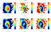 |
Fig. 1 a) NGC 23: PMAS observed (not corrected for extinction or underlying stellar absoption) maps of emission line ratios: [O iii]λ5007/Hβ (top middle), [O i]λ6300/Hα (top right), [N ii]λ6584/Hα (bottom middle) and [S ii]λλ6717, 6731/Hα (bottom right). Also shown are the maps of the observed Hα flux (top left) and EW(Hα)em (bottom left) of the line in emission. The FoV of the PMAS maps is 16″ × 16″, and the orientation is North up, East to the left. The crosses on the maps mark the peak of the PMAS optical continuum emission at ~6200 Å (see Paper I for details). The Hα maps are shown in a square root scale to emphasize the low surface-brightness regions. |
Statistical properties of the spatially resolved of line emission.
We also produced standard optical diagnostic diagrams using the brightest emission lines (Baldwin et al. 1981; Veilleux & Osterbrock 1987) on a spaxel-by-spaxel basis for the galaxies in our sample. These diagrams provide useful information on the excitation conditions of different regions in galaxies, such as, photoionization by young stars, shocks, and AGN photoionization. In Paper I we presented such diagrams for the nuclear and integrated measurements of our sample. The spatially-resolved diagnostic diagrams for each of the galaxies in our sample are shown in Fig. 2. We also produced [N ii]λ6584/Hα vs. [S ii]λλ6717, 6731/Hα diagrams (Fig. 3) for each of the galaxies in our sample. These diagrams have an advantage over the Veilleux & Osterbrock (1987) diagrams in that they contain more data points, as the [O iii]λ5007/Hβ line ratio can be strongly affected by both the presence of an underlying stellar absorption and extinction. As we shall see in Sects. 5 and 6, the effects of the Balmer absorption stellar features on the observed line ratios are not negligible in regions with low values of EW(Hα)em or EW(Hβ)em. For this reason, the individual measurements in diagrams of Figs. 2 and 3 are color-coded according to arbitrarily chosen ranges of EW(Hα)em. All these diagrams and the effects of the correction for stellar absorption features will be discussed in Sect. 6.
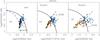 |
Fig. 2 a) Observed diagnostic diagrams for the spatially resolved measurements of NGC 23. The line ratios are not corrected for extinction or underlying stellar absorption. The star symbols are the nuclear region measurements given in Paper I. The line ratios for individual spaxels are color coded according to the value of the EW(Hα)em of the line in emission: green dots EW(Hα)em > 60 Å, orange dots 20 Å < EW(Hα)em ≤ 60 Å, blue dots 5 Å < EW(Hα)em ≤ 20 Å, and red dots EW(Hα)em ≤ 5 Å. The solid lines are the “maximum starburst lines” defined by Kewley et al. (2001) from theoretical modeling, and the thick dashed lines are the empirical separation between AGN and H ii regions of Kauffmann et al. (2003), and between Seyfert and LINERs of Kewley et al. (2006). |
The errors of the line ratios depend on the observed values of EW(Hα)em and the S/N of the spectra. We estimated the typical uncertainties by comparing the line ratios measured automatically with our IDL routines with those fitted manually with the splot routine within IRAF for selected spaxels in each galaxy. For each galaxy, the comparison was made for spaxels within the smallest observed range of EW(Hα)em where the uncertainties are the highest. By choosing spaxels with low values of EW(Hα)em, we basically estimated an upper limit to the uncertainties of the observed line ratios. As can be seen from Fig. 3 the largest uncertainties in the [N ii]λ6584/Hα and [S ii]λλ6717, 6731/Hα ratios are 10−25%, and 15−40%, respectively, depending on the range of EW(Hα)em and the galaxy.
 |
Fig. 3 Spatially resolved observed [N ii]λ6584/Hα vs. [S ii]λλ6717, 6731/Hα diagrams for each of the galaxies in our sample. The individual spaxel measurements are color coded according to EW(Hα)em as in Fig. 2. The spaxels corresponding to the nuclear region are shown as a star-like symbol. The line ratios are not corrected for underlying stellar absorption or extinction. The error bars are the typical uncertainties in the measured line ratios for the smallest range of EW(Hα)em, color-coded as the data points, measured for each galaxy. The uncertainties in the line ratios of spaxels with EW(Hα)em greater than the plotted range are always lower. The solid lines are the Dopita et al. (2006) models for evolving H ii regions for instantaneous star formation and 2 Z⊙ metallicity in all cases except for the MCG +12-02-001, UGC 1845 and MCG +02-20-003 plots where we show the Z⊙ models (see Table 7 for the estimated abundances). The pink, dark blue and light blue lines correspond to log ℛ parameters of −2, −4, and −6. The dashed lines are isochrones for ages 0.1, 0.5, 1, 2 and 3 Myr from top to bottom. The ℛ parameter is defined as the ratio of the mass of the ionizing cluster to the pressure of the interstellar medium. |
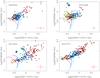 |
Fig. 3 continued. For NGC 7469 and NGC 7591 we identified the nuclear regions as the 4 central brightest spaxels at 6200 Å, as these two galaxies contain an active nucleus and the seeing (FWHM) was larger than the spaxel size. |
2.3. Extraction and analysis of the 1D spectra of selected regions
For each galaxy we extracted the nuclear and integrated spectra as done in Paper I. Briefly, we identified the position of the optical nucleus as the peak of the 6200 Å continuum emission, and extracted the nuclear spectrum using the corresponding spaxel. The physical size covered by the nuclear spectrum for each galaxy was given in Paper I, and it is typically the approximate central 300 pc. The integrated spectrum of each galaxy was extracted by defining ~6200 Å continuum isophotes and then summing up all the spaxels contained within the chosen external continuum isophote to include as much as possible of the PMAS FoV. The area covered by the integrated spectrum can be seen in Fig. 1 in Paper I, and it is generally the central 5−8 kpc, depending on the galaxy.
For the three galaxies observed under photometric conditions: NGC 23, NGC 2388, and NGC 7771, we extracted spectra of a number of bright H ii regions. The locations of the selected regions are shown in the lower panels of Fig. 4. These regions were chosen to probe, for each galaxy, a range of EW(Hα)em and continuum slopes as can be seen from Fig. 5. Veilleux et al. (1995) found that the extinction in (U)LIRGs powered by star formation is correlated with the shape of the optical continuum. We estimated the shape of the optical continuum by measuring the ratio (C6500/C4800) between the continuum fluxes (see Fig. 4) near Hβ and Hα at 4800 and 6500 Å, respectively. The definition of this ratio is given in Table 2. Similarly the gas extinctions are related to the HST/NICMOS F160W−F110W colors (see Alonso-Herrero et al. 2006). Figure 4 shows how the selected H ii regions in these galaxies span a range in F160W to F110W flux ratios, and there is a good correspondence between red near-IR colors and steep optical continua. Table 3 gives details of the observed properties of these regions. Given the good quality of the spectra for these three galaxies, we will use them to do a detailed modeling of the stellar populations in these galaxies (Sect. 3.1).
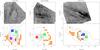 |
Fig. 4 Upper panels: HST/NICMOS 1.6 μm to 1.1μm flux ratio maps. Dark regions show a deficit of 1.1 μm flux, that is, a redder F160W−F110W color. All three galaxies are shown on the same flux ratio scale. Lower panels: the contours are the observed Hα fluxes of the three galaxies for which extracted spectra of circumnuclear H ii regions. For each galaxy we show the regions of interest: the nucleus (defined as the peak of the 6200 Å continuum emission, light blue dots), bright H ii regions (red, blue, purple, and green dots). The orange dots are the spaxels used to produce the average spectrum of regions with relatively low EW of Hα (see Sect. 2.3). For NGC 7771 we additionally extracted a spectrum of the possible location of the true nucleus (shown as a black dot), based on the Hα velocity field (see Paper I for details). |
As we will explain in Sect. 5.1, we can use the 4000 Å-break and the Balmer lines in absorption, and in particular the Hδ line, to infer an estimate of the average age of the stellar populations. Although the Hδ nebular emission line is much weaker than Hα and Hβ, it can also be observed in emission in bright/young H ii regions (see for instance the HII-1 region in NGC 23, Figs. 4 and 5). To minimize the contamination from the Balmer lines in emission, for each galaxy we selected regions with low values of EW(Hα)em so we could attempt to measure the Hδ feature in absorption. We produced the average spectrum of this low EW emission by summing up the spaxels with the specified range of EW(Hα)em for each galaxy. The individual spaxels had typically 20 Å < EW(Hα)em < 6 Å, but the specific range depended on the galaxy and the S/N of the data. From the comparison between the maps of the observed EW(Hα)em in Fig. 1 and the HST/NICMOS Paα maps shown in Paper I, it is clear that the low EW(Hα)em values are associated with regions of diffuse emission or low surface-brightness H ii regions. Table 4 lists the values of EW(Hα)em as measured from the average spectrum of regions of low EW of Hα of each galaxy. All the extracted spectra were shifted to rest-frame wavelengths prior to the analysis and fitting the stellar populations.
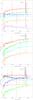 |
Fig. 5 PMAS spectra of selected regions (see Fig. 3 and Table 3), arbitrarily scaled, of the three galaxies observed under photometric conditions: NGC 23, NGC 2388, and NGC 7771. The color used for plotting the spectra corresponds to those of Fig. 4 (lower panel). |
In Sect. 5 we will study the stellar populations of LIRGs using the 4000 Å-break and the Hδ stellar feature. We adopted the definition of Balogh et al. (1999) for the Dn(4000) index and that of Worthey & Ottaviani (1997) for the HδA index2. We measured these indices for the nuclear and integrated spectra, as well as the average spectra of regions of low EW(Hα)em. The pseudo-continuum bands of these two indices, as well as the line window for the HδA index are listed in Table 2. For the majority of the selected H ii regions (see Table 3), as well as the nuclei and integrated emission (Table 4), the measured values HδA are only lower limits as the observed values of EW(Hα)em in emission imply a contribution from nebular Hδ emission to the index. In Tables 3 and 4 we marked those regions where we clearly detected the nebular Hδ line in emission within the stellar absorption. We also measured the Hα flux and the EW(Hα)em of the line in emission in all the extracted spectra.
3. Modeling of the stellar populations
As discussed in Paper I the nuclear and integrated spectra of our sample of LIRGs show evidence of the presence of an ionizing stellar population, plus a more evolved stellar population as indicated by the presence of strong absorption stellar features in the blue part of the spectrum. This is also apparent for the H ii regions in our sample of LIRGs, including those with the highest values of EW(Hα)em (see Fig. 5). These strong absorption stellar features appear to be a general property of local LIRGs and ULIRGs (see e.g., Armus et al. 1989; Veilleux et al. 1995; Kim et al. 1995, 1998; Marcillac et al. 2006; Chen et al. 2009; Rodríguez Zaurín et al. 2009), as well as intermediate-redshift LIRGs (see e.g., Hammer et al. 2005; Marcillac et al. 2006; Caputi et al. 2008). Moreover, it has been suggested that LIRGs represent phases in the life of galaxies with episodic and extremely efficient star formation (Hammer et al. 2005). This suggests that using one single stellar population (SSP) may not be appropriate for modeling individual regions and the integrated emission of LIRGs.
3.1. Modeling of the stellar continuum
For the modeling of the stellar continuum we used the Bruzual & Charlot (2003, BC03 hereafter) models with solar metallicity, instantaneous star formation, and a Salpeter (Salpeter 1955) initial mass function (IMF) with lower and upper mass cutoffs of ml = 0.1 M⊙ and mu = 100 M⊙, respectively. These models have a spectral resolution of 3 Å across the whole wavelength range from 3200 to 9500 Å. Using these assumptions we generated template spectra covering ages of between 1 Myr and 10 Gyr. The outputs of these models are normalized to a total mass of 1 M⊙ formed in the burst of star formation. The dust attenuation was modeled using the Calzetti et al. (2000) extinction law, which is appropriate for starburst galaxies.
To fit the optical spectra of the selected regions (see Sect. 2.3) we used the CONFIT code (Robinson et al. 2000), which assumes two stellar populations plus a power law in some cases. Briefly, CONFIT fits the continuum shape of the extracted spectra using a minimum χ2 technique. For each spectrum, CONFIT measures the flux in ~50−70 wavelength bins, chosen to be as evenly distributed in wavelength as possible, and to avoid strong emission lines and atmospheric absorption features (see Rodríguez Zaurín et al. 2009, for details). The relative flux calibration error of 10% measured was assumed during the modeling.
For this work we used a large number of combinations of two stellar populations to determine which stellar populations dominate the optical emission of our galaxies. We divided the two stellar populations into an ionizing stellar population (<20 Myr, in intervals of 1, 2, ... 10, 20 Myr) with a varying reddening (E(B − V)young ≤ 2.0 in increasing steps of 0.1) and an evolved stellar population with ages between 100 Myr and 10 Gyr (100, 300, 500, 700 Myr; 1, 2, ... 5 Gyr and 10 Gyr) with moderate reddening (E(B − V)evolved = 0,0.2,0.4). This preferential dust extinction is based on the scenario where the youngest stellar populations are still partially embedded in their dusty birth places, whereas the more evolved stellar populations have already moved away from their natal clouds (Calzetti et al. 1994). Poggianti & Wu (2000) demonstrated that this scenario was compatible with the observed optical spectra of infrared bright galaxies.
The choice of an ionizing population is driven by the fact that all the spectra modeled in this paper show Hα in emission with EW(Hα)em > 7 Å (except for the nuclear region of IC 860, see Tables 3 and 4), which sets an upper limit to the age of approximately 10−20 Myr for an instantaneous burst (see e.g., Leitherer et al. 1999, and below). We did not include very old stellar populations ( > 10 Gyr) because these do not appear to have a strong contribution to the optical light of local LIRGs and ULIRGs (see e.g., Chen et al. 2009; Rodríguez Zaurín et al. 2009). We assumed that both stellar populations were formed in instantaneous bursts, which seems an appropriate assumption because the physical scales of the selected regions are a few hundred parsecs (see Table 3) and contain, at most, a few H ii regions, as shown in Paper I.
A priori, fits with  should be considered acceptable fits to the overall shape of the continuum (see discussion in Tadhunter et al. 2005). However, the absolute value of
  is strongly dependent on the estimated errors. We found that combinations with
  produced poor fits to the overall shape of the continuum. Moreover, for most regions we found acceptable solutions for
  , where
  was the minimum value of for a given region. Out of these solutions, we selected the best fitting models based on a visual inspection of the fits to those absorption features with relatively little emission line contamination. These include high order Balmer lines, the CaII K λ3934 line, the G-band λ4305, and the MgIb λ5173 band. Finally, we rejected solutions with ages of the young ionizing stellar populations older than the upper limits (that is, before subtracting the stellar continuum produced by the evolved stars) set by the EW(Hα)em values (see Sect. 3.2).
3.2. Modeling of the hydrogen recombination emission lines
To model the properties of the hydrogen recombination emission lines, we used the Starburst99 model (Leitherer et al. 1999) with the same IMF and metallicity assumptions as above to generate the time evolution of EW(Hα)em (and also for Hβ) for an instantaneous burst of star formation. This model is better qualified for the modeling of populations containing hot massive stars (see Vázquez & Leitherer 2005, for details). The EW of the Hα emission line resulting from subtracting the modeled continuum arising from the non-ionizing stellar population from the observed spectra can be used to put further constraints on the age (tneb) of the ionizing stellar populations. Additionally, we used the Hα/Hβ emission line ratio measured after subtracting the stellar continuum (from both the ionizing and non-ionizing stellar populations) to provide an independent estimate of the extinction to the gas (E(B − V)neb). This gas is ionized by the young stellar population assumed in the previous section.
4. The maps of the EW(Hα)em and optical line ratios
The maps of EW(Hα)em for our sample of LIRGs, covering on average the central ~4.7 kpc are shown in Fig. 1. The map of NGC 7771 covers the central ~7.7 kpc × 4.4 kpc. To first order the EW of the nebular Balmer emission lines can be used as indicators of the age of the ionizing stellar populations. The values of EW(Hα)em in our sample of LIRGs (see Fig. 1), except for the nuclear region of IC 860 (Table 4), indicate ages of the young stellar populations of between 5 and ~10−20 Myr (see e.g., Leitherer et al. 1999, and Sect. 3.1). For the majority of the LIRGs in this sample, as well as for our VLT/VIMOS LIRGs of Rodríguez Zaurín et al. (2010b), the highest values of the EW of Hα are not coincident with the peak of the optical continuum (the nucleus). However, it is important to note that the EW of the Balmer nebular emission lines are also sensitive to the mass of the underlying non-ionizing population. In this sense, the EW of the Balmer emission lines also provide an estimate of the ratio of the current star formation rate compared with the averaged past star formation, that is, the burst strength (see e.g., Kennicutt et al. 1987; Alonso-Herrero et al. 1996), whether this refers to the integrated emission of a galaxy or to individual regions within galaxies. In cases of low burst strengths, the observed values of the EW only provide upper limits to the age of the current star formation burst. Thus, the most likely explanation for the lower nuclear EW(Hα)em, when compared to those of circumnuclear H ii regions observed in some galaxies, is a larger contribution from the underlying (more evolved) stellar population (see Kennicutt et al. 1989) and/or a slightly more evolved stellar population.
The regions with the highest values of EW(Hα)em show values of the [N ii]λ6584/Hα and [S ii]λλ6717, 6731/Hα line ratios (see Fig. 1) typical of H ii regions in normal star-forming galaxies. In contrast, most nuclear regions in our LIRGs tend to show slightly greater lines ratios than the H ii regions of the same galaxy. This is clearly seen in the diagnostic diagrams of Fig. 2 where for each galaxy we plot the spatially resolved (on a spaxel by spaxel basis) line ratios as a function of the observed value of EW(Hα)em in emission. This is in line with findings for the nuclei and H ii regions in normal star forming galaxies (see e.g., Kennicutt et al. 1989). We note, however, that the line ratios of regions with low EW(Hα)em will have the largest corrections for the presence of stellar Balmer absorption lines as we shall see in Sect. 6.2.
The presence of extra-nuclear regions with enhanced values of the [N ii]λ6584/Hα and [S ii]λλ6717, 6731/Hα ratios relative to those of H ii regions is again a common property not only of the LIRGs studied here, but also of our VLT/VIMOS sample of LIRGs (see Monreal-Ibero et al. 2010a) and our WHT/INTEGRAL sample of ULIRGs (see García-Marín et al., in prep.). In our sample of LIRGs these regions tend to be associated with diffuse emission rather than with high surface-brightness H ii regions, as is also the case for normal and starburst galaxies (Wang et al. 1998). Moreover, for our VLT/VIMOS sample of LIRGs Monreal-Ibero et al. (2010a) found a correlation between the enhanced optical ratios and increasing gas velocity dispersion in interacting and merger LIRGs, and this correlation is attributed to the presence of shocks associated with the interaction processes. Our PMAS sample is mostly composed of isolated galaxies and weakly interacting galaxies (see Paper I), and thus it is unlikely these processes are responsible for the enhanced line ratios. However, because the majority of the regions with enhanced [N ii]λ6584/Hα and [S ii]λλ6717, 6731/Hα ratios in our sample are observed in regions of relatively low EW(Hα)em, we will postpone the discussion of this issue after the line ratios are corrected for the presence of underlying Balmer stellar absorption features (see Sect. 6.2).
Definition of indices of the stellar absorption features.
5. The stellar populations of local LIRGs
5.1. Results using the 4000 Å break and Balmer line absorption features
Kauffmann et al. (2003) used a method based on the 4000 Å-break and the Balmer Hδ feature in absorption to constrain the mean (light-weighted) age of the stellar population of a galaxy and the mass fraction formed in recent bursts of star formation. Therefore, this method provides information about the light-averaged properties of the stellar populations. From the stellar continuum spectra generated with BC03, we measured the Dn(4000) and the HδA indices (see Sect. 2.3, and Table 2 for definitions of the indices). For an instantaneous burst of star formation the Dn(4000) index increases monotonically with the age of the stellar population, while the depth of the Hδ line absorption feature increases until about 300−400 Myr after the burst, and then decreases again (black line in Fig. 6). Thus the presence of high order Balmer lines in absorption is usually interpreted as the signature of an intermediate age (100 Myr−1Gyr) stellar population. The evolution of these two indices is shown in Fig. 6 using the BC03 models and is similar to the results of Kauffmann et al. (2003a) and González-Delgado et al. (2005).
As discussed in Sect. 3, we need a combination of (at least) two stellar populations to reproduce the observed properties of LIRGs, including the Dn(4000) and HδA indices. This is clear from Fig. 6, where a single stellar population formed in an instantaneous burst (black line) does not reproduce the observed indices of the nuclei and regions of low-EW(Hα)em in our sample of LIRGs. A model with a constant star formation rate predicts Dn(4000) < 1.2 for all ages (see Fig. 21 of Caputi et al. 2008), and thus it is not appropriate for our galaxies either.
Figure 6 shows the result of combining two stellar populations. In this diagram, the choice of the age of the ionizing stellar population is not critical because Dn(4000) and HδA do not vary much during approximately the first ~10−20 Myr of the evolution of a single stellar population formed in an instantaneous burst (see e.g., González-Delgado et al. 2005). Thus with this kind of diagrams we cannot constrain the age of the youngest stellar populations in LIRGs. As we shall see in Sect. 5.2, the combined modeling of the stellar continuum and the nebular emission lines puts strong constraints on the properties of the ionizing stellar population. In Fig. 6 we then combined a 10 Myr population with evolved stellar populations with ages of 700 Myr, 1 Gyr, 2 Gyr, 3 Gyr, and 5 Gyr. The ages of the evolved stellar population are based on the location in this diagram of the observed values for the nuclei and regions of low-EW(Hα)em in our sample of LIRGs. A scenario where the evolved stellar population was formed in an instantaneous burst and the current star formation is taking place at a constant rate (see Sarzi et al. 2007, for Dn(4000) vs. HδA diagrams generated under this assumption) would underpredict the strength of the Hδ absorption feature for most of the selected regions in our LIRGs, as was the case for the star-forming regions in nuclear rings in the sample of Sarzi et al. (2007).
From Fig. 6 it is clear that the main effect of combining a young population and an evolved 1−2 Gyr stellar population is the change in the observed value of the Dn(4000) index, which becomes smaller as the fraction in mass of the young stellar population increases. For a combination with a younger evolved stellar population (~700 Myr) the effect is observed in both indices, as is the case for older evolved populations (> 2 Gyr). Based on this figure and taking into account that the measured HδA are lower limits, the age of the evolved stellar population is between 1 and 3 Gyr for most of the galaxies in our sample. The only exception is NGC 7771 that appears to show the presence of an intermediate age (700 Myr–1 Gyr) stellar population. We also show in Fig. 6 a range of mass fractions for the young stellar population, which in general are relatively low for the nuclei and regions of low-EW(Hα)em.
In Fig. 7 we show the effects on the Dn(4000) vs. HδA diagram from the combination of a reddened young stellar population and an unreddened evolved population. Figure 7 clearly demonstrates that not accounting for the extinction to the young stellar population would make us underestimate its mass fraction as well as underestimate the age of the evolved stellar population. However, it is also apparent from Figs. 6 and 7, that it is not possible to disentangle the effects of extinction, ages of the stellar populations, and mass contributions from this kind of diagrams alone.
Observed properties of selected star-forming regions.
Observed properties for the nuclei, average of regions with low EW(Hα)em and integrated emission.
5.2. Results of the modeling of the stellar continuum and nebular emission
As explained in Sect. 2.3, we selected a number of regions in our sample of LIRGs for the study of their stellar populations. These include the nuclear regions, the average spectra of regions of low-EW(Hα)em, as well as a number of bright H ii regions in NGC 23, NGC 2388, and NGC 7771. We excluded from this analysis three galaxies for various reasons. The nuclear optical spectra of MCG +12-02-001 appears to be completely dominated by a young ionizing stellar population (that is, we do not see absorption features), and thus it was not possible to constrain the evolved stellar population. The signal-to-noise ratio of the nuclear spectrum of UGC 1845 did not allow us to constrain the properties of the stellar populations. Finally we excluded NGC 7469 because of the possible contamination of the optical spectra from the AGN non-stellar continuum. We refer the reader to Díaz-Santos et al. (2007) for a detailed study of the stellar populations of the ring of star formation of NGC 7469 using high angular resolution HST photometric data.
Table 5 summarizes for each galaxy and region the acceptable ranges of ages and extinctions for the evolved (tevolved and E(B − V)evolved) and ionizing (tyoung and E(B − V)young) stellar populations derived from the stellar continuum fit as explained in Sect. 3.1. We also list in this table the fraction of the light in the normalising bin emitted by the ionizing (young) stellar component (fNB), for the models that produce adequate fits. Because of the different shapes of the extracted spectra it was not always possible to select the same normalizing bin. However, the normalizing bin was always selected to be located within the wavelength range of 4400−4800 Å and usually spanning ~100 Å. Fig. 8 presents a few examples of fits to the stellar continuum for a number of regions in our sample.
For the majority of the regions studied here except for the optical nucleus of NGC 7771 (see Sect. 5.2.1), we find that stellar populations with ages between 100 Myr and 500 Myr do not make a strong contribution to the optical light. Ages for the evolved stellar populations of between 0.7 and 5 Gyr (or even 10 Gyr in some cases) provided reasonable fits to the optical continua. These ages are within the range of ages derived for massive spiral galaxies (Gallazzi et al. 2005, and references therein). Another noteworthy result is that the regions with low-EW(Hα)em in the galaxies tend to have slightly older ionizing stellar populations and less extinction than other regions for the same galaxy. The ages of the evolved stellar populations agree with our findings in the previous section using the Dn(4000) and HδA diagram, keeping in mind that HδA may only provide a lower limit to the age of the evolved stars for some of the regions. We finally note that for models including evolved plus young stellar components it is particularly hard to distinguish between ages in the range 2−10 Gyr. Therefore, in some cases we are not able to put strong constraints on the age of the stellar populations for ages older than ~1−2 Gyr.
As can be seen from Table 5 the ionizing stellar populations always contribute a minimum of fNB ≥ 15% to the optical emission in all the modeled spectra, and they dominate the emission (fNB ≥ 50%) in, at least, 7 of the 23 spectra modeled. On the other hand, in the nuclear regions of NGC 23 and IC 860, and NGC 7771, the evolved stellar populations may be the main contributors to the optical light (see also Table 6). Our spectra do not sample the near-UV spectral region, which is important for constraining the properties of the ionizing stellar populations. Therefore, the ages of such stellar populations are not well constrained when fitting the stellar continuum alone.
We were able to put tighter constraints on the young stellar populations when we included the nebular fitting. Table 6 gives the parameters of the stellar continuum and nebular fits for those regions shown in Fig. 8. The nebular ages and extinctions (tneb and E(B − V)neb) were derived as explained in Sect. 3.2, for an acceptable combination of stellar populations close or at the minimum value of . We find ages of the ionizing stellar populations from the EW of Hα of between 5.6 and 8.8 Myr. The extinctions to the ionizing stellar stars range between E(B − V) = 0.2 and E(B − V) = 1.8 (Tables 5 and 6). The extinctions to the ionizing stellar populations are always significantly greater than those to the evolved stars, and generally consistent with those derived to the young stars from the stellar continuum modeling.
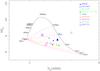 |
Fig. 6 Dn(4000) vs. HδA diagram. The small symbols are the measurements from the average spectrum of the regions with low EW(Hα)em of each LIRG, whereas the large symbols are the measurements corresponding to the nuclear regions (see Table 4). For NGC 7591 we plot the values corresponding to the integrated spectrum. Note that in the majority of nuclei the HδA indices are lower limits due to possible contamination from the nebular Hδ emission line. The black solid line is the time evolution (from 1 Myr to 5 Gyr) as predicted by the BC03 models using solar metallicity, a Salpeter IMF, and an instantaneous burst of star formation. The dashed lines are combinations of different evolved populations (ages 700 Myr, 1 Gyr, 2 Gyr, 3 Gyr, and 5 Gyr) and a young stellar population of 10 Myr. The dotted lines represent the fraction in mass of young stars with values of 0.001, 0.002, 0.005, 0.008, 0.01, 0.02, 0.05, 0.08, 0.1, 0.2, 0.5, and 0.8, from right to left. |
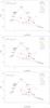 |
Fig. 7 Same as Fig. 6, but showing the effects of reddening the young stellar population with E(B − V)young = 0.2 (upper panel), E(B − V)young = 0.5 (middle panel), and E(B − V)young = 1 (bottom panel), and using the Calzetti et al. (2000) extinction law. |
Ranges of ages, extinctions and light fractions from young stars as derived from the stellar continuum modeling.
Our results are, in a broad brush sense, consistent with those of Rodríguez Zaurín et al. (2009) for their sample of ULIRGs. That is, the optical spectra can be modeled using a combination of an evolved plus a young stellar population. However, the extracted spectra of our LIRGs show, in most cases, deeper G and Mg ib bands than those of the ULIRGs of the Rodríguez Zaurín et al. (2009) sample. This suggests that the evolved stellar populations are somewhat older for the LIRGs in our sample. In fact, Rodríguez Zaurín et al. (2009) found adequate fits for their ULIRGs which included evolved stellar populations of 0.3−0.5 Gyr, while this was rarely the case for our sample of LIRGs. The stellar populations dominating the optical light of ULIRGs could be the result of enhanced star formation coinciding with the first pass of the merging nuclei, along with a further, more intense, episode of star formation occurring as the nuclei finally merge together (Rodríguez Zaurín et al. 2010a). Our sample of LIRGs on the other hand, is mostly composed of relatively isolated spiral galaxies and weakly interacting galaxies (see Paper I), with moderate IR luminosities (see Sect. 2.1). Given the relatively low fraction of strongly interacting/merger systems in our sample compared to the Rodríguez Zaurín et al. (2009) ULIRG sample, it may not be unexpected that intermediate-age (~100−500 Myr) stellar populations do not dominate the optical light of our LIRGs. The only exception in our sample are the central regions of NGC 7771 (see discussion in Sect. 5.2.2). Moderate luminosity spiral-like LIRGs may be constantly forming stars and may have not undergone a major burst of star formation in the last 1−2 Gyr, as is the case of normal spiral galaxies (Kauffmann et al. 2003b). Our results are also in accord with the observational findings of Poggianti & Wu (2000) that most isolated systems in their sample of IR-bright galaxies showed on average more moderate Balmer absorption features than the interacting systems. The effects of possible minor mergers are likely to be difficult to evaluate using the stellar populations as models and observations suggest that it is the satellite galaxy rather than the primary galaxy that is more susceptible to enhanced star formation (Woods & Geller 2007; Cox et al. 2008).
5.2.1. The central regions of NGC 7771
There is dynamical evidence that NGC 7771 is weakly interacting with NGC 7770 (Keel 1993) and is located in a group of galaxies. It is then possible that the interaction process resulted in a strong burst of star formation in the past. For instance, the ring in this galaxy, clearly detected in our Paα images (see Paper I), appears to have a complex star formation history with evidence of multiple generations of stars (Davies et al. 1997; Smith et al. 1999; Reunanen et al. 2000).
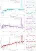 |
Fig. 8 a) Examples of fits to the stellar continuum of regions in our sample of galaxies. The bluest rest-frame wavelength used for the modeling is 3800 Å. For each region, the left panel shows the observed spectrum (thick color line) and the model spectrum (thin black line) in arbitrary units. The spectra are normalized to unity at a wavelength within the normalizing bin (4400−4800 Å). The model parameters for each region are given at the top right of each plot. The right panels are blow-ups of some spectral regions of interest. We mark the high order Balmer lines as well as Hδ, Hγ, and, Hβ as dotted lines. The Ca ii H and Ca ii K lines (lower right panel), the G-band (middle right panel), and the Mg ib band (upper right panel) are marked as thick solid lines. The spectral resolution of the BC03 models has been slightly degraded to match approximately that of our PMAS spectra. |
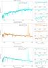 |
Fig. 8 b) Same as Fig. 8a. For the nuclear region of NGC 7771 we also show the positions of the He i features at 3820, 4026, 4388, and 4471 Å. |
The optical nucleus of NGC 7771 is the only region in our sample of LIRGs for which adequate fits were obtained with a large contribution to the optical light from an intermediate-age (300−500 Myr) stellar population (see Table 5 and Fig. 8). The fit to the average spectrum of regions with low EW(Hα)em also required an evolved stellar population of 500−700 Myr. In the case of the nuclear spectrum there is the need for an additional stellar population based on the presence of He i absorption features at various wavelengths, which are indicated in Fig. 8b. These absorption lines are strongest for stellar populations with ages in the range 20−50 Myr (González-Delgado et al. 1999, 2005), and are not observed in stellar populations older than 100 Myr (the lifetime of B stars). The presence of this important population of non-ionizing stars dominated by B stars was already infered by Davies et al. (1997). Given that there is evidence that B stars are present, for this region we also tried combinations including stellar populations of 30−80 Myr for the young component. We found that a combination with a dominant (fNB = 70−80%), low reddening (E(B − V)young ~ 0.2) stellar population of 40−50 Myr plus an unreddened evolved stellar population of few Gyr provided an acceptable fit. We note that with this combination the stellar population responsible for ionizing the gas is not accounted for. Therefore, in this particular case, it is likely that models including a larger number of stellar components (at least three) would be more adequate. We again emphasize that the nuclear region of NGC 7771 is the only region where we find a clear evidence of these He i features. In this respect, it is not clear if the optical nucleus of this galaxy may be a special region in this galaxy (see Davies et al. 1997, for a discussion of this issue). It is important to recall at this point that the optical nucleus of NGC 7771 is probably not the true nucleus of the galaxy, as it does not coincide with the center of the bright ring of star formation, the peak of near-IR emission (see Paper I), or even with the region with the highest value of EW(Hα)em (see Fig. 1j).
Examples of stellar continuum and nebular modeling.
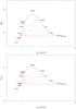 |
Fig. 9 Theoretical Dn(4000) vs. HβA (upper panel) and Dn(4000) vs. HαA (lower panel) diagrams. The black solid line is the time evolution (from 1 Myr to 5 Gyr) as predicted by the BC03 models using solar metallicity, a Salpeter IMF, and an instantaneous burst of star formation. The dashed lines are combinations of different evolved populations (ages 700 Myr, 1 Gyr, 2 Gyr, 3 Gyr, and 5 Gyr) and a young ionizing stellar population of 6 Myr. The dotted lines represent the contribution in mass of the two stellar populations, as in Fig. 6. |
5.3. Predictions for the Hβ and Hα stellar absorption features
To study in detail the optical line ratios and in particular those of the diffuse regions, we need to correct for the presence of Hβ and Hα stellar absorption features. However, given the strong star formation activity in our sample, it is difficult to measure reliably these absorption features because of the strong contamination produced by the Balmer recombination lines in emission. An alternative approach is to generate theoretical diagrams of Dn(4000) vs. HαA and Dn(4000) vs. HβA measured from the spectra generated from the combination of the BC03 young and evolved stellar populations as explained in Sect. 3.1. The HβA and HαA indices for the stellar absorption features are defined in a similar way to that used for the Hδ absorption feature (see Sect. 2.3), and thus have a positive value. The line windows, and the blue and red pseudo-continuum windows defined by González Delgado et al. (2005) are given in Table 1. For the ages of the evolved stellar population we used those derived in Sect. 5.2. For the ionizing stellar population we chose an age of 6 Myr, which is representative of our sample of LIRGs (Tables 5 and 6), although the results are not strongly dependent of chosen age of this population. For the mass fractions we used the same values as those shown in Fig. 6.
From the Dn(4000) vs. HβA diagram (Fig. 9, upper panel), we can see that for ages of the evolved stellar population of between 1 and 5 Gyr, the predicted average value of the HβA index is ~5 ± 1 Å. This value is almost independent of the mass fraction in young stars, except for cases where the stellar mass is dominated by the contribution from ionizing stars. For NGC 7771, which is the clearest case in our sample for the presence of an intermediate age stellar population, the predicted value would be HβA ~ 7 ± 1 Å. In this case, the predicted value is more sensitive to the mass in young stars and the age of the evolved stellar population. For comparison, the measurements of HβA reported by Kim et al. (1995) for the central 2 kpc of the galaxies in common with our sample are 3 and 6 Å, although Kim et al. (1995) pointed out these values were admittedly subjective because of the method they used for fitting their data.
Figure 9 (lower panel) shows the predictions for the Dn(4000) vs. HαA diagram. In the case of HαA there is little dependence of the predicted value with the mass fraction in young stars. For the majority of our LIRGs with ages of the stellar population 1−5Gyr the average predicted value for the index would be HαA ~ 3 ± 0.5 Å, whereas for NGC 7771 we would predict HαA ~ 4 ± 0.5 Å. For comparison, Moustakas & Kennicutt (2006b) found an average Hα stellar absorption correction of 2.8 ± 0.4 Å for the integrated spectra of a sample of nearby star forming galaxies.
6. Excitation conditions in local LIRGs
6.1. Spatially resolved diagnostic diagrams
Diagnostic diagrams using bright optical emission lines (Balwin et al. 1981; Veilleux & Osterbrock 1987) are useful for differentiating between the various sources of excitation of the gas in the nuclei of galaxies and their integrated emission. With optical IFS data we can additionally study the distribution of the ionization structure of spatially resolved regions (that is, on a spaxel-by-spaxel basis) of nearby galaxies (e.g., García-Marín et al. 2006, in prep.; García-Lorenzo et al. 2008; Blanc et al. 2009; Stoklasová et al. 2009; Monreal-Ibero et al. 2010b), as well as of H ii regions in nearby galaxies (e.g., Relaño et al. 2010). The diagnostic diagrams for the spatially resolved measurements for each of the LIRGs in our sample are shown in Fig. 2. The measurements for the individual spaxels are color coded according to the observed value of the EW(Hα)em in emission. In these diagrams we plotted the empirical and theoretical boundaries derived by Kauffmann et al. (2003c) and Kewley et al. (2001). These boundaries are shown for reference as they may provide clues about the dominant excitation mechanism: ionization by young stars, shocks, or AGN ionization.
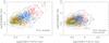 |
Fig. 10 Spatially resolved [N ii]λ6584/Hα vs. [S ii]λλ6717, 6731/Hα diagrams for the full PMAS sample. The individual measurements (a total of 1852 spaxels) in both panels are color coded according to the observed EW(Hα)em in emission as in Fig. 2. The left panel shows the ratios not corrected for underlying Hα stellar absorption, whereas the right panel are the line ratios corrected for underlying Hα stellar absorption as described in Sect. 5.3. The contours are plotted to help assess the data point density in bins of 0.1 dex in both emission line ratios. |
The first result worth noticing is that a large number of the spatially resolved measurements in the [O iii]λ5007/Hβ vs. [N ii]λ6584/Hα diagram (Fig. 2, left panels) fall in the composite region, and in particular a large number of those spaxels with EW(Hα)em < 20 Å. A similar result is found for ULIRGs (García-Marín et al., in prep.). On the other hand, most of the spaxels with EW(Hα)em > 60Å are located in the H ii region of the diagram, with the only exception of some regions in NGC 7469. There are also differences from galaxy to galaxy. For instance the majority of the spaxels of MCG +12-02-001 and NGC 5936 are located in the H ii region of the diagram, while other cases such as UGC 1845 most spaxels are in the composite region. The composite region on this diagram lies between the observational AGN/H ii boundary and the “maximum starburst line” of Kewley et al. (2001), above which the observed line ratios cannot be explained by star formation alone. Kewley et al. (2006) interpreted the observed ratios in the composite region as produced by a metal-rich stellar population and an AGN (but see Cid Fernandes et al. 2010 and references therein, for an opposing point of view). While the Kewley et al. argument is valid for nuclear and even integrated spectra of galaxies, in our sample a large number of spaxels with enhanced line ratios are detected in the extra-nuclear regions of galaxies without an AGN.
The number of spatially resolved measurements located in the LINER region of the diagrams of the other two diagnostic diagrams (Fig. 2, middle and right panels), is lower than in the diagram with the [N ii]λ6584/Hα ratio (see also Veilleux et al. 1995). This is in part a sensitivity issue, especially for the relatively faint [O i]λ6300 line, which is, on the other hand, a very good shock tracer. Still, a large number of spaxels with EW(Hα)em < 20Å, mostly in NGC 23, MCG+02-20-003, and NGC 7771, are in the LINER region of these two diagnostic diagrams. The presence of extra-nuclear regions in LIRGs and ULIRGs with LINER-like excitation has often been interpreted as an indication for the presence of large scale shocks where interactions are playing a major role (Monreal-Ibero et al. 2006, 2010a) or to shocks due to the presence of outflowing nuclear gas (see e.g., Armus et al. 1989). Calzetti et al. (2004) using a [O iii]λ5007/Hβ vs. [S ii]λλ6717, 6731/Hα diagram with spatially resolved measurements of four nearby starburst galaxies, found evidence that there is non-photoionized gas. These authors also demonstrated that shocks from supernovae and stellar winds are able to provide sufficient mechanical energy to account for the non-photoionized gas in their galaxies. In the case of this sample of LIRGs, most galaxies do not show evidence strong interactions either from their morphologies or from the observed Hα velocity fields (see Paper I). Our LIRGs, however present very high central Hα surface brightnesses and thus star formation rates per surface area (see Alonso-Herrero et al. 2006), which would imply a contribution from supernovae. One important caveat to keep in mind is that the observed line ratios in the diagnostic diagrams of Fig. 2 have not been corrected for the presence of stellar absorption. These corrections will be most relevant for those spaxels with the lowest equivalent widths of the hydrogen recombination emission lines, as we shall see in the following section.
6.2. Spatially resolved [N II]λ6584 /Hα vs. [S II]λλ6717, 6731/Hα diagrams
In our own Galaxy and other galaxies enhanced [N ii]λ6584/Hα and [S ii]λλ6717, 6731/Hα line ratios appear to be associated with the presence of diffuse ionized gas (DIG3, see the recent review by Haffner et al. 2009, and references therein). The presence of DIG emission has been detected spectroscopically in the extra-planar emission of edge-on galaxies (Rand 1996; Miller & Veilleux 2003). A similar result was infered based on the enhanced low-ionization emission relative to that of H ii regions of the integrated emission of galaxies (see e.g., Lehnert & Heckman 1994; Wang et al. 1997; Moustakas & Kennicutt 2006a) as well as on spatially resolved measurements (see e.g., Calzetti et al. 2004). In Paper I we already discussed the possibility of the presence of this diffuse emission in our sample of LIRGs, as in general the integrated line ratios of the galaxies are greater than the typical values observed in disk H ii regions (see Kennicutt et al. 1989). Moreover, the regions of enhanced line ratios in our LIRGs are generally not associated with regions of high Paα surface brightness, that is, bright H ii regions. Clear examples of this are NGC 23, NGC 7591 and NGC 7771 (see Fig. 1 and Paper I). Regions of enhanced low ionization emission can also be associated to the presence of an AGN in the form of an ionization cone, as is the case of one of the nuclei of the interacting LIRG Arp 299 (García-Marín et al. 2006).
To study in more detail the excitation conditions in our sample of LIRGs, we produced spatially resolved [S ii]λλ6717, 6731/Hα vs. [N ii]λ6584/Hα diagrams for each of the galaxies (see Fig. 3). The advantages of these diagrams over the standard diagnostic diagrams are twofold. First they contain more data points than the diagnostic diagrams (see the statistics in Table 1 for the number of spaxels with measurements for each line ratio) because Hβ in LIRGs is heavily affected by extinction and stellar absorption. Second, as we showed in Sect. 5.3, the corrections for the presence of stellar absorption in Hα are less dependent on the results of the stellar population models than those for Hβ.
A comparison between the observed [S ii]λλ6717, 6731/Hα vs. [N ii]λ6584/Hα ratios and predictions from different models (ionization by young stars, shocks, AGN photoionization) can shed some light on the dominant excitation conditions in our sample of LIRGs. In Fig. 3 we show the Dopita et al. (2006) models for evolving H ii regions. In these models the ionization parameter is replaced by the ℛ parameter, which is defined as the ratio of the mass of the ionizing cluster to the pressure of the interstellar medium. We chose models with solar and twice solar metallicity based on the derived abundances of our galaxies from the integrated line ratios over the central few kpc (Paper I) corrected for stellar absorption (see Sect. 5.3). To estimate the abundances, we used the Pettini & Pagel (2004) empirical calibration based on the [O iii]λ5007/Hβ and [N ii]λ6584/Hα ratios, also known as the O3N2 index (see Alloin et al. 1979). All the LIRGs in our sample have near solar or super-solar abundances (see Table 7), for a solar abundance of 12 + log (O/H) = 8.66 (Asplund et al. 2004), and are within the derived abundances of the large sample of LIRGs studied by Rupke et al. (2008).
Although we do not intend to use the Dopita et al. models for dating the H ii regions, it is clear that line ratios of [S ii]λλ6717, 6731/Hα ~ 0.6−1 could be produced by evolved and metal rich H ii regions (see details in Dopita et al. 2006). As can be seen from Fig. 3, the [S ii]λλ6717, 6731/Hα vs. [N ii]λ6584/Hα diagrams of the central regions of some galaxies (e.g., MCG+12-02-001 and NGC 5936) could be mostly explained as emission coming from H ii regions, although it has to be noted that there are no spaxels with EW(Hα)em < 5Å in the central regions of these galaxies. On the other hand, galaxies like NGC 23, NGC 7591 and NGC 7771 show a significant numbers of spaxels with EW(Hα)em < 20 Å whose line ratios (not corrected for stellar absorption) cannot be explained by the Dopita et al. (2006) H ii region models. Shock models such as those of Allen et al. (2008) could explain line ratios log ([N ii]λ6584/Hα) > −0.7 and log ([S ii]λλ6717, 6731/Hα) > −0.7. These models are not plotted in Fig. 3, but see Fig. 8 of Monreal-Ibero et al. (2010a) and a discussion by Miller & Veilleux (2003).
To get a more global picture of the excitation conditions in LIRGs, in Fig. 10 (left panel) we plot a [N ii]λ6584/Hα vs. [S ii]λλ6717, 6731/Hα diagram for the full PMAS sample, showing a total number of 1852 spaxels again color coded in terms of EW(Hα)em in emission. It is clear from this figure that those spaxels with the lowest EW(Hα)em tend to show the highest values of the line ratios, indicating that in part the enhanced values are due to the presence of Hα stellar absorption. The right panel of Fig. 10 shows the same diagram after correcting statistically each spaxel for the presence of Hα in absorption, with the average values of HαA derived in Sect. 5.3. The effect of correcting the emission line ratios for stellar absorption in our sample is evident, especially for spaxels with EW(Hα)em < 20Å. However, as can be seen from the histograms in Fig. 11, even after the correction for stellar absorption there is still a significant number of spaxels with enhanced line ratios. For example, after correction for stellar absorption approximately 25% of the spaxels show log ([S ii]λλ6717, 6731/Hα) > −0.2, which is the highest line ratio allowed by the 2 Z⊙ Dopita et al. (2006) models. This suggests that there are other mechanisms apart from young stars ionizing the gas in our sample of LIRGs.
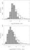 |
Fig. 11 Histograms showing the distributions of the spatially resolved [N ii]λ6584/Hα (upper panel) and [S ii]λλ6717, 6731/Hα (lower panel) line ratios for the full PMAS sample, for a total of 1852 spaxels. The thick line empty histograms are the observed line ratios, while the thin line filled histograms are the line ratios corrected for stellar absorption. |
We can now compare our observations with those of Monreal-Ibero et al. (2010a) for the VLT/VIMOS sample of LIRGs. The VIMOS sample was observed with a mean spatial sampling of 270 pc per spaxel, which is similar to that of the PMAS data. The Monreal-Ibero et al. (2010a) sample contains galaxies chosen to probe the different morphologies observed in LIRGs from relatively isolated galaxies, to interacting galaxies to mergers. In that study we found that the median value of the [N ii]λ6584/Hα ratios measured on a spaxel-by-spaxel basis has a very weak dependence with the morphology of the system. The distributions of the [S ii]λλ6717, 6731/Hα and the [O i]λ6300/Hα ratios, on the other hand, tend to be more enhanced for galaxies classified as interacting and mergers. Our PMAS sample is smaller than the VIMOS sample, but it is representative of the LIRG class, in the sense that it comprises the majority of the IRAS RBGS LIRGs at d < 75 Mpc that can be observed from Calar Alto. As such, the PMAS sample is mostly composed of LIRGs with relatively low IR luminosities, and thus dominated by isolated spiral galaxies or systems in weak interaction (see also Sanders & Ishida 2004). The median values of the line ratios (on a spaxel-by-spaxel basis) in the PMAS sample corrected for stellar absorption are [N ii]λ6584/Hα = 0.45 and [S ii]λλ6717, 6731/Hα = 0.44 (see also Fig. 11). For the statistics we used only spaxels with measurements of both line ratios. These ratios are comparable to, although slightly greater than, those measured by Monreal-Ibero et al. (2010a) for the VLT/VIMOS sample of LIRGs. The slight difference may be due to the fact that the PMAS data probe more regions (spaxels) with low EW(Hα)em than in the VLT/VIMOS sample (see Rodríguez Zaurín et al. 2010b). This in turn results in the PMAS data being more sensitive to diffuse emission.
6.3. Diffuse emission
Regardless of the main mechanism responsible for exciting the diffuse gas in galaxies (e.g., massive stars, escaping photons from H ii regions, shocks), it is clear that quantifying the fraction of diffuse emission in galaxies is important for understanding issues such as the early reionization of the universe. Traditionally the fraction of diffuse emission in galaxies was obtained by identifying and doing photometry of H ii regions, to separate the emission coming from H ii regions from that of the DIG (see e.g., Zurita et al. 2000; Oey et al. 2007, see review by Haffner et al. 2009). The main results from this method were that the mean fraction of diffuse emission in galaxies was 50−60% with no correlation with the Hubble morphological type (Thilker et al. 2002; Oey et al. 2007). However, Oey et al. (2007) found that starburst galaxies showed lower fractions of diffuse Hα emission when compared to other galaxies.
Abundances and fraction of diffuse ionized emission in the central regions of LIRGs.
In Alonso-Herrero et al. (2006) we measured the Paα fluxes of H ii regions, and estimated the total Paα fluxes using HST/NICMOS narrow band images, for similar FoVs to those of the PMAS data. Due to the relatively small FoV of the Paα NICMOS images (NIC2 camera 19″ × 19″) the main uncertainty in measuring Paα fluxes, both in H ii regions and the total (H ii + DIG) emission is the background removal. On the other hand, narrow-band Paα imaging does not suffer from problems associated with contamination by the [N ii] doublet associated with using narrow-band Hα imaging (see Blanc et al. 2009, for a discussion of the issue). For each galaxy we measured the total Paα luminosity over the NICMOS FoV, and converted it to Hα flux assuming case B recombination (Hα/Paα = 8.6, Hummer & Storey 1987). Using the total Hα luminosity and the Hα luminosity in H ii regions given in Table 3 of Alonso-Herrero et al. (2006), we computed the DIG fraction for each galaxy. The DIG fractions are between 8 to 76% (Table 7). The range given for each galaxy takes into account the uncertainties in calculating the total Paα emission from the HST/NICMOS narrow-band imaging (see Alonso-Herrero et al. 2006, for details). The DIG fractions given in this table for each LIRG correspond only to the central few kiloparsecs, as neither the NICMOS nor the PMAS observations cover the full extent of the galaxies.
Alternatively Blanc et al. (2009) computed the DIG fraction in M 51 from optical IFS by comparing the observed [S ii]λ6717/Hα line ratios with the typical values measured for H ii regions and the DIG in the Milky Way (MW) by Madsen et al. (2006), and taking into account the difference in metallicity between M 51 and the MW. The PMAS 1″ spaxel covers approximately 300 pc for the typical distances of our galaxies (Sect. 2.1). Defining the sizes of H ii regions, even at HST resolutions, is not straightforward, but results for LIRGs at distances similar to those of the PMAS sample, indicate typical sizes of ~150−200pc (Alonso-Herrero et al. 2002). We thus expect that each measurement of a given line ratio contains both H ii region and DIG emission, as assumed by the Blanc et al. (2009) method. In the MW the average [S ii]λ6717/Hα line ratios of H ii regions and the diffuse emission are 0.11 ± 0.03 and 0.34 ± 0.13, respectively (Madsen et al. 2006; Blanc et al. 2009). In Table 7 we list the DIG fractions we obtained with the line [S ii]λ6717/Hα ratios corrected for stellar absorption and the Blanc et al. (2009) method. For each galaxy we give a range, with the lowest value corresponding to scaling the MW H ii and DIG ratios to ~1.7 times solar, and the highest ratio for solar metallicity.
Table 7 shows that the fraction of diffuse emission in the central few kpc of our LIRGs varies significantly from galaxy to galaxy. Oey et al. (2007) found that starburst galaxies, defined as galaxies having Hα surface brightnesses above 2.5 × 1039 ergs-1kpc-2 within the Hα half radius, have relatively low DIG fractions (<60%), when compared to non-starburst galaxies. According to this definition all our galaxies are starbursts (see Alonso-Herrero et al. 2006), and thus in most cases our DIG fractions are below 60%. The high DIG fraction inferred for NGC 7591 may be explained if some of enhanced line ratios are produced in a narrow line region associated with the AGN in this galaxy. We also find that the fractions of DIG emission in the central few kpc obtained with the two methods described above mostly agree with each other, within the uncertainties (Table 7). We note however, that the line ratio method always tends to provide a lower DIG fraction than the H ii region photometry method (see also Blanc et al. 2009, for M 51). The two LIRGs with the most discrepant fractions using the two methods are NGC 5936 and NGC 7771. In the case of NGC 5936 we attribute the discrepancy to the fact that, except for the very nuclear regions, the other H ii regions in the FoV of the NICMOS images appear quite diffuse (see Alonso-Herrero et al. 2006, and Paper I), and thus the DIG fraction estimated from the NICMOS Paα images is clearly just an upper limit. In the case of NGC 7771, even if we applied the lower correction for the Hα absorption feature (that is, if the evolved stellar population had an age of a few Gyr), the DIG fraction from the [S ii]λ6717/Hα line ratios would be in the range of 3 to 13%. The most likely explanation is that the faintest H ii regions just outside the bright ring of star formation were not identified in the NICMOS Paα images, and this resulted in an overestimate of the diffuse emission.
7. Summary
This is the second paper of a series presenting a PMAS IFS study of 11 local (average distance of 61 Mpc) LIRGs covering the central few kiloparsecs of the galaxies. We selected the galaxies from the complete volume-limited sample of LIRG of Alonso-Herrero et al. (2006), which has an average IR luminosity of log (LIR/L⊙) = 11.32. As such, our sample of LIRGs is mostly composed of isolated spiral galaxies, galaxies with companions, and weakly interacting galaxies. The PMAS observations covered a spectral range of 3700−7200 Å, with a spectral resolution of 6.8 Å (FWHM). We used a 1″-size spaxel that provides a typical physical sampling of approximately 300 pc. The PMAS observations were complemented with our own existing HST/NICMOS observations of the near-infrared continuum and the Paα emission line. We combined the spectral information provided by the PMAS IFS and the spatial information provided by the HST/NICMOS observations to study in detail the stellar populations, the excitation conditions of the gas, and diffuse emission in local LIRGs.
To study the stellar populations we selected the nuclear regions of each galaxy, as well as a number of bright H ii regions in NGC 23, NGC 2388, and NGC 7771. We also extracted for each galaxy, when possible, the average spectrum of regions with low values of EW(Hα)em. These regions were selected such that they did not contain high surface-brightness H ii regions to minimize the contamination by hydrogen nebular emission in the stellar absorption features. We used BC03 and Starburst99 to fit the stellar continuum and the nebular emission, respectively. For the modeling we assumed two stellar populations formed in instantaneous bursts with a Salpeter IMF and solar metallicity. The PMAS maps of EW(Hα)em in our sample of LIRGs (see Fig. 1), except for the nuclear region of IC 860 (Table 4), indicate ages of the young stellar populations of between 5 and ~10−20 Myr (see e.g., Leitherer et al. 1999, and Sect. 3.1). We thus chose ages of the ionizing stellar populations of between 1 and 20 Myr, and ≥100 Myr for the evolved one. Both stellar populations were extinguished with a range of values of E(B − V).
Combinations of evolved stellar populations with ages between 0.7 and 5−10 Gyr with relatively low extinctions, and ionizing stellar populations with higher extinctions provided reasonable fits to the optical continua of most of our regions. The spectra of our LIRGs tend to show deeper MgIb and G-bands than the ULIRGs in the Rodríguez Zaurín et al. (2010a) sample. This suggests that the stellar populations in our sample are somewhat older. In fact, we found little evidence of a strong contribution to the optical light from intermediate-aged stellar populations with ages of ~100−500 Myr in our sample of LIRGs. The only exception in our sample is NGC 7771. Several of the regions studied in this galaxy, including its optical nucleus, show clear indications for an important contribution from an intermediate-aged stellar population (~100−700 Myr). Additionally the optical nucleus of NGC 7771 contains a large number of stars with ages in the range 30−50 Myr, as indicated by the presence of strong He i absorption features.
The majority of the selected regions in our sample of LIRGs have a significant contribution to the 4600 Å continuum light from the ionizing stellar populations, and for about one-third the ionizing stellar populations have a dominant contribution. The ages of the evolved stellar populations of our LIRGs are within the ranges observed in massive spiral galaxies. The fitting of the stellar continuum and the nebular properties yielded ages of the ionizing stellar populations of between 5 and 9 Myr, and extinctions in the range E(B − V)young = 0.2−1.8. The extinctions from the stellar continuum fits and the Balmer decrement agree with each other, and tend to be higher than those required for the evolved stellar populations.
We used the brightest emission lines to study the spatially resolved (on a spaxel-by-spaxel basis) excitation conditions in the central few kiloparsecs of our sample of LIRGs. When using traditional diagnostic diagrams involving bright optical emission lines, the location of the spatially-resolved line ratios varies from LIRG to LIRG. Some galaxies have most of their spaxels in the H ii region of the diagnostic diagrams, while others have spaxels located both in the H ii and LINER regions of the diagrams. In particular, a significant number of spaxels with EW(Hα)em < 20Å have enhanced [N ii]λ6584/Hα, [S ii]λλ6717, 6731/Hα and [O i]λ6300/Hα line ratios, when compared to those of H ii regions. These spaxels tend to be associated with regions of diffuse Hα and Paα emission in these galaxies, that is, they do not coincide with high surface-brightness H ii regions identified in the HST/NICMOS Paα images.
We also produced spatially resolved [S ii]λλ6717, 6731/Hα vs. [N ii]λ6584/Hα diagrams for each of the galaxies, and the full PMAS sample. These diagrams have the advantage of containing more data points than the traditional diagnostic diagrams, and of having lower corrections for the presence of Hα stellar absorption than diagrams using Hβ. Even so, the corrections for stellar absorption to the observed line ratios are significant for spaxels with EW(Hα)em < 20 Å. After the correction for stellar absorption, there is still a significant number of spaxels in these diagrams whose line ratios cannot be explained as produced entirely by photoionization by young stars (e.g., log [S ii]λλ6717, 6731/Hα > −0.2). These enhanced ratios are probably due to the combined contributions of H ii region emission and DIG emission.
We estimated the fraction of DIG emission in the central few kiloparsecs of our LIRG using two different methods. The first one used H ii region photometry from the NICMOS Paα images. The second method was based on the comparison of the spatially-resolved [S ii]λ6717/Hα line ratios of our LIRGs, and those of the MW H ii regions and DIG. The DIG fractions over the central few kiloparsecs vary from galaxy to galaxy, but are generally <60%, as found for starburst galaxies by Oey et al. (2007).
Online material
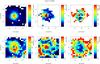 |
Fig. 1 h) As Fig. 1a but for NGC 7469. The Hβ and Hα measurements correspond to the narrow component of the lines (see Paper I for details). |
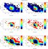 |
Fig. 1 j) As Fig. 1a but for NGC 7771, except that the FoV for this galaxy covers the central 28″ × 16″ (Sect. 2.1 for details). The maps are shown: Hα flux (top left), EW(Hα)em (top right), [O iii]λ5007/Hβ (middle left), [O i]λ6300/Hα (middle right), [N ii]λ6584/Hα (bottom left) and [S ii]λλ6717, 6731/Hα (bottom right). |
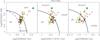 |
Fig. 2 h) As Fig. 2a but for NGC 7469. The Hβ and Hα measurements correspond to the narrow component of the lines (see Paper I for details). |
http://www.purl.com/net/mpfit developed by Markwardt (2008).
We note that the value of this index is positive for absorption, and throughout this paper we will use this symbol to indicate the feature in absorption.
This gas is also referred to as diffuse ionized medium or DIM, and warm ionized medium or WIM.
Acknowledgments
We thank an anonymous referee for useful suggestions that helped improve the paper. We thank C. Tadhunter, G. Blanc and F. Rosales for enlightening discussions. We are grateful to the Calar Alto staff, and in particular to S. Sánchez, A. Guijarro, L. Montoya, and N. Cardiel, for their support during the PMAS observing campaigns.
This research has made use of the NASA/IPAC Extragalactic Database (NED) which is operated by the Jet Propulsion Laboratory, California Institute of Technology, under contract with the National Aeronautics and Space Administration.
A.A.-H., J.R.-Z., L.C., and S.A. acknowledge support from the Spanish Plan Nacional del Espacio under grant ESP2007-65475-C02-01. A.A.-H. also acknowledges support for this work from the Spanish Ministry of Science and Innovation through Proyecto Intramural Especial under grant number 200850I003. M.G.-M. is supported by the German Federal Department of Education and Research (BMBF) under project numbers: 50OS0502 and 50OS0801. A.M.-I. is supported by the Spanish Ministry of Science and Innovation (MICINN) under program “Specialization in International Organisms”, ref. ES2006-0003.
References
- Allen, M. G., Groves, B. A., Dopita, M. A., Sutherland, R. S., & Kewley, L. J. 2008, ApJS, 178, 20 [Google Scholar]
- Alloin, D., Collin-Souffrin, S., Joly, M., Vigroux, L., et al. 1979, A&A, 78, 200 [NASA ADS] [Google Scholar]
- Alonso-Herrero, A., Aragón-Salamanca, A., Zamorano, J., & Rego, M. 1996, MNRAS, 278, 417 [NASA ADS] [Google Scholar]
- Alonso-Herrero, A., Rieke, G. H., Rike, M. J., & Scoville, N. Z. 2002, AJ, 124, 166 [NASA ADS] [CrossRef] [Google Scholar]
- Alonso-Herrero, A., Rieke, G. H., Rieke, M. J., et al. 2006, ApJ, 650, 835 [NASA ADS] [CrossRef] [Google Scholar]
- Alonso-Herrero, A., García-Marín, M., Monreal-Ibero, A., et al. 2009, A&A, 506, 1541 (Paper I) [NASA ADS] [CrossRef] [EDP Sciences] [Google Scholar]
- Armus, L., Heckman, T. M., & Miley, G. K. 1989, ApJ, 347, 727 [NASA ADS] [CrossRef] [Google Scholar]
- Arribas, S., Carter, D., Cavaller, L., et al. 1998, SPIE, 3355, 821 [NASA ADS] [CrossRef] [Google Scholar]
- Arribas, S., Colina, L., & Clements, D. 2001, ApJ, 560, 160 [NASA ADS] [CrossRef] [Google Scholar]
- Arribas, S., Colina, L., Monreal-Ibero, A., et al. 2008, A&A, 479, 687 [NASA ADS] [CrossRef] [EDP Sciences] [Google Scholar]
- Asplund, M., Grevesse, N., Sauval, A. J., Allen de Prieto, C., & Kiselman, D. 2004, A&A, 417, 751 [NASA ADS] [CrossRef] [EDP Sciences] [Google Scholar]
- Baldwin, J. A., Phillips, M. M., & Terlevich, R. 1981, PASP, 93, 5 [NASA ADS] [CrossRef] [EDP Sciences] [Google Scholar]
- Balogh, M. L., Morris, S. L., Yee, H. K. C., Carlberg, R. G., & Ellingson, E. 1999, ApJ, 527, 54 [NASA ADS] [CrossRef] [Google Scholar]
- Bedregal, A. G., Colina, L., Alonso-Herrero, A., & Arribas, S. 2009, ApJ, 698, 1852 [NASA ADS] [CrossRef] [Google Scholar]
- Bingham, R. G., Gellatly, D. W., Jenkins, C. R., & Worswick, S. P. 1994, Proc. SPIE, 2198, 56 [NASA ADS] [CrossRef] [Google Scholar]
- Blanc, G. A., Heiderman, A., Gebhardt, K., Evans, N. J. II, & Adams, J. 2009, ApJ, 704, 842 [NASA ADS] [CrossRef] [Google Scholar]
- Bruzual, G., & Charlot, S. 2003, MNRAS, 344, 1000 (BC03) [NASA ADS] [CrossRef] [Google Scholar]
- Bushouse, H. A., Borne, K. D., Colina, L., et al. 2002, ApJS, 138, 1 [NASA ADS] [CrossRef] [Google Scholar]
- Calzetti, D., Kinney, A. L., & Storchi-Bergmann, T. 1994, ApJ, 429, 582 [NASA ADS] [CrossRef] [Google Scholar]
- Calzetti, D., Armus, L., Bohlin, R. C., et al. 2000, ApJ, 533, 682 [NASA ADS] [CrossRef] [Google Scholar]
- Calzetti, D., Harris, J., Gallagher, J. S., III, et al. 2004, AJ, 127, 1405 [NASA ADS] [CrossRef] [Google Scholar]
- Caputi, K. I., Lilly, S. J., Aussel, H., et al. 2008, ApJ, 680, 939 [NASA ADS] [CrossRef] [Google Scholar]
- Chen, X. Y., Liang, Y. C., Hammer, F., Zhao, Y. H., & Zhong, G. H. 2009, A&A, 495, 457 [NASA ADS] [CrossRef] [EDP Sciences] [Google Scholar]
- Cid Fernandes, R., Stasińska, G., Schlickmann, M. S., et al. 2010, MNRAS, 403, 1036 [NASA ADS] [CrossRef] [Google Scholar]
- Colina, L., Arribas, S., & Borne, K. D. 1999, ApJ, 527, L13 [NASA ADS] [CrossRef] [PubMed] [Google Scholar]
- Colina, L., Arribas, S., & Monreal-Ibero, A. 2005, ApJ, 621, 725 [NASA ADS] [CrossRef] [Google Scholar]
- Cox, T. J., Jonsson, P., Somerville, R. S., Primack, J. R., & Dekel, A. 2008, MNRAS, 384, 386 [NASA ADS] [CrossRef] [Google Scholar]
- Davies, R. I., Alonso-Herrero, A., & Ward, M. J. 1997, MNRAS, 291, 557 [NASA ADS] [Google Scholar]
- Díaz-Santos, T., Alonso-Herrero, A., Colina, L., Ryder, S. D., & Knapen, J. H. 2007, ApJ, 661, 149 [NASA ADS] [CrossRef] [Google Scholar]
- Dopita, M. A., Fischera, J., Sutherland, R. S., et al. 2006, ApJS, 167, 177 [NASA ADS] [CrossRef] [Google Scholar]
- Gallazzi, A., Charlot, S., Brinchmann, J., White, S. D., & Tremonti, C. A. 2005, MNRAS, 362, 41 [NASA ADS] [CrossRef] [Google Scholar]
- Gao, Y., & Solomon, P. M. 2004, ApJS, 152, 63 [NASA ADS] [CrossRef] [Google Scholar]
- García-Lorenzo, B., Cairs, L. M., Caon, N., Monreal-Ibero, A., Kehrig, C., et al. 2008, ApJ, 677, 201 [NASA ADS] [CrossRef] [Google Scholar]
- García-Marín, M., Colina, L., Arribas, S., Alonso-Herrero, A., & Mediavilla, E. 2006, ApJ, 650, 850 [NASA ADS] [CrossRef] [Google Scholar]
- García-Marín, M., Colina, L., & Arribas, S. 2009a, A&A, 505, 1017 [NASA ADS] [CrossRef] [EDP Sciences] [Google Scholar]
- García-Marín, M., Colina, L., Arribas, S., & Monreal-Ibero, A. 2009b, A&A, 505, 1319 [NASA ADS] [CrossRef] [EDP Sciences] [Google Scholar]
- Goldader, J. D., Joseph, R. D., Doyon, R., & Sanders, D. B. 1995, ApJ, 444, 97 [NASA ADS] [CrossRef] [Google Scholar]
- González Delgado, R. M., Leitherer, C., & Heckman, T. M. 1999, ApJS, 125, 489 [NASA ADS] [CrossRef] [Google Scholar]
- GonzálezDelgado, R. M., Cerviño, M., Martins, L. P., Leitherer, C., & Hauschildt, P. H. 2005, MNRAS, 357, 945 [NASA ADS] [CrossRef] [Google Scholar]
- Graciá-Carpio, J., Burillo, S., García-Burillo, S., Planesas, P., Colina, L., et al. 2006, ApJ, 640, L135 [NASA ADS] [CrossRef] [Google Scholar]
- Graciá-Carpio, J., Burillo, S., García-Burillo, S., Planesas, P., Fuente, A., Usero, A., et al. 2008, A&A, 479, 703 [NASA ADS] [CrossRef] [EDP Sciences] [Google Scholar]
- Haffner, L. M., Dettmar, R.-J., Beckman, J. E., et al. 2009, RvMP, 81, 969 [Google Scholar]
- Hammer, F., Flores, H., Elbaz, D., et al. 2005, A&A, 430, 115 [NASA ADS] [CrossRef] [EDP Sciences] [Google Scholar]
- Heckman, T. M., Armus, L., & Miley, G. K. 1987, AJ, 92, 276 [NASA ADS] [CrossRef] [Google Scholar]
- Heckman, T. M., Lehnert, M. D., Strickland, D. K., Armus, L. 2000, ApJS, 129, 493 [NASA ADS] [CrossRef] [MathSciNet] [Google Scholar]
- Hummer, D. G., & Storey, P. J. 1987, MNRAS, 224, 801 [NASA ADS] [CrossRef] [Google Scholar]
- Kauffmann, G., Heckman, T. M., White, S. D. M., et al. 2003a, MNRAS, 341, 33 [NASA ADS] [CrossRef] [Google Scholar]
- Kauffmann, G., Heckman, T. M., White, S. D. M., et al. 2003b, MNRAS, 341, 54 [Google Scholar]
- Kauffmann, G., Heckman, T. M., Tremonti, C., et al. 2003c, MNRAS, 346, 1055 [Google Scholar]
- Keel, W. C. 1993, AJ, 106, 1771 [NASA ADS] [CrossRef] [Google Scholar]
- Kehrig, C., Vílchez, J. M., Sánchez, S. F., et al. 2008, A&A, 477, 813 [NASA ADS] [CrossRef] [EDP Sciences] [Google Scholar]
- Kennicutt, R. C. Jr., Keel, W. C., van der Hulst, J. M., Hummel, E., & Roettiger, K. A. 1987, AJ, 93, 1011 [NASA ADS] [CrossRef] [Google Scholar]
- Kennicutt, R. C. Jr., Keel, W., C., & Blaha, C. A. 1989, AJ, 97, 1022 [NASA ADS] [CrossRef] [Google Scholar]
- Kewley, L. J., Dopita, M. A., Sutherland, R. S., Heisler, C. A., & Trevena, J. 2001, ApJ, 556, 121 [Google Scholar]
- Kewley, L. J., Groves, B., Kauffmann, G., et al. 2006, MNRAS, 372, 961 [NASA ADS] [CrossRef] [Google Scholar]
- Kim, D.-C., Sanders, D. B., Veilleux, S., Mazzarella, J. M., & Soifer, B. T. 1995, ApJS, 98, 129 [NASA ADS] [CrossRef] [Google Scholar]
- Kim, D.-C., Veilleux, S., & Sanders, D. B. 1998, ApJ, 508, 627 [NASA ADS] [CrossRef] [Google Scholar]
- Le Fèvre, O., Saisse, M., Mancini, D., et al. 2003, SPIE, 4841, 1670 [Google Scholar]
- Lehnert, M. D., & Heckman, T. M. 1994, ApJ, 426, L27 [NASA ADS] [CrossRef] [Google Scholar]
- Leitherer, C., Schaerer, D., Goldader, J. D., et al. 1999, ApJS, 123, 3 [NASA ADS] [CrossRef] [Google Scholar]
- Lípari, S., Mediavilla, E., Garcia-Lorenzo, B., et al. 2004a, MNRAS, 355, 641 [NASA ADS] [CrossRef] [Google Scholar]
- Lípari, S., Mediavilla, E., Daz, R. J., et al. 2004b, MNRAS, 348, 369 [NASA ADS] [CrossRef] [Google Scholar]
- Madsen, G. J., Reynolds, R. J., & Haffner, L. M. 2006, ApJ, 652, 401 [NASA ADS] [CrossRef] [Google Scholar]
- Marcillac, D., Elbaz, D., Charlot, S., et al. A. 2006, A&A, 458, 369 [NASA ADS] [CrossRef] [EDP Sciences] [Google Scholar]
- Markwardt, C. B. 2008, Non-Linear Least Squares Fitting in IDL with MPFIT, in proc. Astronomical Data Analysis Software and Systems XVIII, Quebec, Canada, eds. D. Bohlender, P. Dowler & D. Durand (Astronomical Society of the Pacific: San Francisco), ASP Conf. Ser., 411, 251 [Google Scholar]
- Miller, S. T., & Veilleux, S. 2003, ApJ, 592, 79 [NASA ADS] [CrossRef] [Google Scholar]
- Monreal-Ibero, A., Arribas, S., Colina, L., Rodríguez Zaurín, J., Alonso-Herrero, A., & García-Marín, M. 2010a, A&A, 517, A28 [NASA ADS] [CrossRef] [EDP Sciences] [Google Scholar]
- Monreal-Ibero, A., Vílchez, J. M., Walsh, J. R., & Muñón-Tuñón, C. 2010b, A&A, 517, A27 [NASA ADS] [CrossRef] [EDP Sciences] [Google Scholar]
- Monreal-Ibero, A., Arribas, S., & Colina, L. 2006, ApJ, 637, 138 [NASA ADS] [CrossRef] [Google Scholar]
- Moustakas, J., & Kennicutt, R. C. Jr. 2006a, ApJ, 651, 155 [NASA ADS] [CrossRef] [Google Scholar]
- Moustakas, J., & Kennicutt, R. C. Jr. 2006b, ApJS, 164, 81 [NASA ADS] [CrossRef] [Google Scholar]
- Oey, M. S., Meurer, G. R., Yelda, S., et al. 2007, ApJ, 661, 801 [NASA ADS] [CrossRef] [Google Scholar]
- Pereira-Santaella, M., Alonso-Herrero, A., Rieke, G. H., et al. 2010, ApJS, 188, 447 [NASA ADS] [CrossRef] [Google Scholar]
- Pettini, M., & Pagel, B. E. J. 2004, MNRAS, 348, L59 [NASA ADS] [CrossRef] [Google Scholar]
- Poggianti, B. M., & Wu, H. 2000, ApJ, 529, 157 [NASA ADS] [CrossRef] [Google Scholar]
- Rand, R. J. 1996, ApJ, 462, 712 [CrossRef] [Google Scholar]
- Relaño, M., Monreal-Ibero, A., Vílchez, J. M., & Kennicutt, R. C. 2010, MNRAS, 402, 1635 [NASA ADS] [CrossRef] [Google Scholar]
- Reunanen, J., Kotilainen, J. K., Laine, S., Ryder, S. D., et al. 2000, ApJ, 529, 853 [NASA ADS] [CrossRef] [Google Scholar]
- Reunanen, J., Tacconi-Garman, L. E., & Ivanov, V. D. 2007, MNRAS, 382, 951 [NASA ADS] [CrossRef] [Google Scholar]
- Rigopoulou, D., Spoon, H. W. W., Genzel, R., et al. 1999, AJ, 118, 2625 [NASA ADS] [CrossRef] [Google Scholar]
- Robinson, T., Tadhunter, C., Axon, D., & Robinson, A. 2000, MNRAS, 317, 922 [NASA ADS] [CrossRef] [Google Scholar]
- Rodríguez Zaurín, J., Tadhunter, C. N., & González-Delgado, R. M. 2009, MNRAS, 400, 1139 [NASA ADS] [CrossRef] [Google Scholar]
- Rodríguez Zaurín, J., Tadhunter, C. N., González Delgado, R. M., et al. 2010a, MNRAS, 403, 1317 [NASA ADS] [CrossRef] [Google Scholar]
- Rodríguez Zaurín, J., Arribas, S., Monreal, Ibero, A., et al. 2010b, A&A, in press [arXiv:1009.0112] [Google Scholar]
- Roth, M. M., Kelz, A., Fechner, T., et al. 2005, PASP, 117, 620 [NASA ADS] [CrossRef] [Google Scholar]
- Rupke, D. S. B., Veilleux, S., & Baker, A. J. 2008, ApJ, 674, 172 [NASA ADS] [CrossRef] [Google Scholar]
- Salpeter, E. 1955, ApJ, 121, 161 [Google Scholar]
- Sanders, D. B., & Mirabel, I. F. 1996, ARA&A, 34, 749 [NASA ADS] [CrossRef] [Google Scholar]
- Sanders, D. B., & Ishida, C. M. 2004, ASPC, 320, 230 [NASA ADS] [Google Scholar]
- Sanders, D. B., Scoville, N. Z., & Soifer, B. T. 1991, ApJ, 370, 158 [NASA ADS] [CrossRef] [Google Scholar]
- Sanders, D. B., Mazzarella, J. M., Kim, D.-C., Surace, J. A., & Soifer, B. T. 2003, AJ, 126, 1607 [Google Scholar]
- Sarzi, M., Allard, E. L., Knapen, J. H., & Mazzuca, L. M. 2007, MNRAS, 380, 949 [NASA ADS] [CrossRef] [Google Scholar]
- Scoville, N. Z., Evans, A. S., Thompson, R., et al. 2000, AJ, 119, 991 [NASA ADS] [CrossRef] [Google Scholar]
- Smith, D. A., Herter, T., Haynes, M. P., Neff, S. G. et al. 1999, ApJ, 510, 669 [NASA ADS] [CrossRef] [Google Scholar]
- Stoklasová, I., Ferruit, P., Emsellem, E., et al. 2009, A&A, 500, 1287 [NASA ADS] [CrossRef] [EDP Sciences] [Google Scholar]
- Tadhunter, C. N., Robinson, T. G., González Delgado, M. R., Wills, K., & Morganti, R. 2005, MNRAS, 356, 480 [NASA ADS] [CrossRef] [Google Scholar]
- Thilker, D. A., Walterbros, R. A. M., Braun, R., & Hoopes, C. G. 2002, AJ, 124, 3118 [NASA ADS] [CrossRef] [Google Scholar]
- Vázquez, G. A., & Leitherer, C. 2005, ApJ, 621, 695 [NASA ADS] [CrossRef] [Google Scholar]
- Veilleux, S., & Osterbrock, D. E. 1987, ApJS, 63, 295 [NASA ADS] [CrossRef] [Google Scholar]
- Veilleux, S., Kim, D.-C., Sanders, D. B., Mazzarella, J. M., & Soifer, B. T. 1995, ApJS, 98, 171 [NASA ADS] [CrossRef] [Google Scholar]
- Veilleux, S., Kim, D.-C., & Sanders, D. B. 1999, ApJ, 522, 113 [NASA ADS] [CrossRef] [Google Scholar]
- Veilleux, S., Kim, D.-C., & Sanders, D. B. 2002, ApJS, 143, 315 [NASA ADS] [CrossRef] [Google Scholar]
- Wang, J., Heckman, T. M., & Lehnert, M. D. 1997, ApJ, 491, 114 [NASA ADS] [CrossRef] [Google Scholar]
- Wang, J., Heckman, T. M., & Lehnert, M. D. 1998, ApJ, 509, 93 [NASA ADS] [CrossRef] [Google Scholar]
- Wood, D. F., & Geller, M. J. 2007, AJ, 134, 527 [NASA ADS] [CrossRef] [Google Scholar]
- Worthey, G., & Ottaviani, D. L. 1997, ApJS, 111, 377 [NASA ADS] [CrossRef] [Google Scholar]
- Wu, H., Zou, Z. L., Xia, X. Y., & Deng, Z. G. 1998, A&AS, 132, 181 [Google Scholar]
- Yuan, T.-T., Kewley, L. J., & Sanders, D. B. 2010, ApJ, 709, 884 [NASA ADS] [CrossRef] [Google Scholar]
- Zurita, A., Rozas, M., & Beckman, J. E. 2000, A&A, 363, 9 [NASA ADS] [Google Scholar]
All Tables
Observed properties for the nuclei, average of regions with low EW(Hα)em and integrated emission.
Ranges of ages, extinctions and light fractions from young stars as derived from the stellar continuum modeling.
Abundances and fraction of diffuse ionized emission in the central regions of LIRGs.
All Figures
|
Fig. 1 a) NGC 23: PMAS observed (not corrected for extinction or underlying stellar absoption) maps of emission line ratios: [O iii]λ5007/Hβ (top middle), [O i]λ6300/Hα (top right), [N ii]λ6584/Hα (bottom middle) and [S ii]λλ6717, 6731/Hα (bottom right). Also shown are the maps of the observed Hα flux (top left) and EW(Hα)em (bottom left) of the line in emission. The FoV of the PMAS maps is 16″ × 16″, and the orientation is North up, East to the left. The crosses on the maps mark the peak of the PMAS optical continuum emission at ~6200 Å (see Paper I for details). The Hα maps are shown in a square root scale to emphasize the low surface-brightness regions. |
| In the text | |
|
Fig. 2 a) Observed diagnostic diagrams for the spatially resolved measurements of NGC 23. The line ratios are not corrected for extinction or underlying stellar absorption. The star symbols are the nuclear region measurements given in Paper I. The line ratios for individual spaxels are color coded according to the value of the EW(Hα)em of the line in emission: green dots EW(Hα)em > 60 Å, orange dots 20 Å < EW(Hα)em ≤ 60 Å, blue dots 5 Å < EW(Hα)em ≤ 20 Å, and red dots EW(Hα)em ≤ 5 Å. The solid lines are the “maximum starburst lines” defined by Kewley et al. (2001) from theoretical modeling, and the thick dashed lines are the empirical separation between AGN and H ii regions of Kauffmann et al. (2003), and between Seyfert and LINERs of Kewley et al. (2006). |
| In the text | |
|
Fig. 3 Spatially resolved observed [N ii]λ6584/Hα vs. [S ii]λλ6717, 6731/Hα diagrams for each of the galaxies in our sample. The individual spaxel measurements are color coded according to EW(Hα)em as in Fig. 2. The spaxels corresponding to the nuclear region are shown as a star-like symbol. The line ratios are not corrected for underlying stellar absorption or extinction. The error bars are the typical uncertainties in the measured line ratios for the smallest range of EW(Hα)em, color-coded as the data points, measured for each galaxy. The uncertainties in the line ratios of spaxels with EW(Hα)em greater than the plotted range are always lower. The solid lines are the Dopita et al. (2006) models for evolving H ii regions for instantaneous star formation and 2 Z⊙ metallicity in all cases except for the MCG +12-02-001, UGC 1845 and MCG +02-20-003 plots where we show the Z⊙ models (see Table 7 for the estimated abundances). The pink, dark blue and light blue lines correspond to log ℛ parameters of −2, −4, and −6. The dashed lines are isochrones for ages 0.1, 0.5, 1, 2 and 3 Myr from top to bottom. The ℛ parameter is defined as the ratio of the mass of the ionizing cluster to the pressure of the interstellar medium. |
| In the text | |
|
Fig. 3 continued. For NGC 7469 and NGC 7591 we identified the nuclear regions as the 4 central brightest spaxels at 6200 Å, as these two galaxies contain an active nucleus and the seeing (FWHM) was larger than the spaxel size. |
| In the text | |
|
Fig. 4 Upper panels: HST/NICMOS 1.6 μm to 1.1μm flux ratio maps. Dark regions show a deficit of 1.1 μm flux, that is, a redder F160W−F110W color. All three galaxies are shown on the same flux ratio scale. Lower panels: the contours are the observed Hα fluxes of the three galaxies for which extracted spectra of circumnuclear H ii regions. For each galaxy we show the regions of interest: the nucleus (defined as the peak of the 6200 Å continuum emission, light blue dots), bright H ii regions (red, blue, purple, and green dots). The orange dots are the spaxels used to produce the average spectrum of regions with relatively low EW of Hα (see Sect. 2.3). For NGC 7771 we additionally extracted a spectrum of the possible location of the true nucleus (shown as a black dot), based on the Hα velocity field (see Paper I for details). |
| In the text | |
|
Fig. 5 PMAS spectra of selected regions (see Fig. 3 and Table 3), arbitrarily scaled, of the three galaxies observed under photometric conditions: NGC 23, NGC 2388, and NGC 7771. The color used for plotting the spectra corresponds to those of Fig. 4 (lower panel). |
| In the text | |
|
Fig. 6 Dn(4000) vs. HδA diagram. The small symbols are the measurements from the average spectrum of the regions with low EW(Hα)em of each LIRG, whereas the large symbols are the measurements corresponding to the nuclear regions (see Table 4). For NGC 7591 we plot the values corresponding to the integrated spectrum. Note that in the majority of nuclei the HδA indices are lower limits due to possible contamination from the nebular Hδ emission line. The black solid line is the time evolution (from 1 Myr to 5 Gyr) as predicted by the BC03 models using solar metallicity, a Salpeter IMF, and an instantaneous burst of star formation. The dashed lines are combinations of different evolved populations (ages 700 Myr, 1 Gyr, 2 Gyr, 3 Gyr, and 5 Gyr) and a young stellar population of 10 Myr. The dotted lines represent the fraction in mass of young stars with values of 0.001, 0.002, 0.005, 0.008, 0.01, 0.02, 0.05, 0.08, 0.1, 0.2, 0.5, and 0.8, from right to left. |
| In the text | |
|
Fig. 7 Same as Fig. 6, but showing the effects of reddening the young stellar population with E(B − V)young = 0.2 (upper panel), E(B − V)young = 0.5 (middle panel), and E(B − V)young = 1 (bottom panel), and using the Calzetti et al. (2000) extinction law. |
| In the text | |
|
Fig. 8 a) Examples of fits to the stellar continuum of regions in our sample of galaxies. The bluest rest-frame wavelength used for the modeling is 3800 Å. For each region, the left panel shows the observed spectrum (thick color line) and the model spectrum (thin black line) in arbitrary units. The spectra are normalized to unity at a wavelength within the normalizing bin (4400−4800 Å). The model parameters for each region are given at the top right of each plot. The right panels are blow-ups of some spectral regions of interest. We mark the high order Balmer lines as well as Hδ, Hγ, and, Hβ as dotted lines. The Ca ii H and Ca ii K lines (lower right panel), the G-band (middle right panel), and the Mg ib band (upper right panel) are marked as thick solid lines. The spectral resolution of the BC03 models has been slightly degraded to match approximately that of our PMAS spectra. |
| In the text | |
|
Fig. 8 b) Same as Fig. 8a. For the nuclear region of NGC 7771 we also show the positions of the He i features at 3820, 4026, 4388, and 4471 Å. |
| In the text | |
|
Fig. 9 Theoretical Dn(4000) vs. HβA (upper panel) and Dn(4000) vs. HαA (lower panel) diagrams. The black solid line is the time evolution (from 1 Myr to 5 Gyr) as predicted by the BC03 models using solar metallicity, a Salpeter IMF, and an instantaneous burst of star formation. The dashed lines are combinations of different evolved populations (ages 700 Myr, 1 Gyr, 2 Gyr, 3 Gyr, and 5 Gyr) and a young ionizing stellar population of 6 Myr. The dotted lines represent the contribution in mass of the two stellar populations, as in Fig. 6. |
| In the text | |
|
Fig. 10 Spatially resolved [N ii]λ6584/Hα vs. [S ii]λλ6717, 6731/Hα diagrams for the full PMAS sample. The individual measurements (a total of 1852 spaxels) in both panels are color coded according to the observed EW(Hα)em in emission as in Fig. 2. The left panel shows the ratios not corrected for underlying Hα stellar absorption, whereas the right panel are the line ratios corrected for underlying Hα stellar absorption as described in Sect. 5.3. The contours are plotted to help assess the data point density in bins of 0.1 dex in both emission line ratios. |
| In the text | |
|
Fig. 11 Histograms showing the distributions of the spatially resolved [N ii]λ6584/Hα (upper panel) and [S ii]λλ6717, 6731/Hα (lower panel) line ratios for the full PMAS sample, for a total of 1852 spaxels. The thick line empty histograms are the observed line ratios, while the thin line filled histograms are the line ratios corrected for stellar absorption. |
| In the text | |
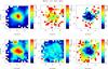 |
Fig. 1 b) As Fig. 1a but for MCG +12-02-001. |
| In the text | |
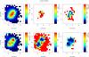 |
Fig. 1 c) As Fig. 1a but for UGC 1845. |
| In the text | |
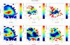 |
Fig. 1 d) As Fig. 1a but for NGC 2388. |
| In the text | |
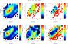 |
Fig. 1 e) As Fig. 1a but for MCG +02-20-003. |
| In the text | |
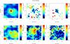 |
Fig. 1 f) As Fig. 1a but for NGC 5936. |
| In the text | |
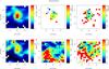 |
Fig. 1 g) As Fig. 1a but for NGC 6701. |
| In the text | |
|
Fig. 1 h) As Fig. 1a but for NGC 7469. The Hβ and Hα measurements correspond to the narrow component of the lines (see Paper I for details). |
| In the text | |
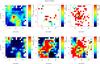 |
Fig. 1 i) As Fig. 1a but for NGC 7591. |
| In the text | |
|
Fig. 1 j) As Fig. 1a but for NGC 7771, except that the FoV for this galaxy covers the central 28″ × 16″ (Sect. 2.1 for details). The maps are shown: Hα flux (top left), EW(Hα)em (top right), [O iii]λ5007/Hβ (middle left), [O i]λ6300/Hα (middle right), [N ii]λ6584/Hα (bottom left) and [S ii]λλ6717, 6731/Hα (bottom right). |
| In the text | |
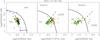 |
Fig. 2 b) As Fig. 2a but for MCG +12-02-001. |
| In the text | |
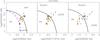 |
Fig. 2 c) As Fig. 2a but for UGC 1845. |
| In the text | |
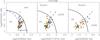 |
Fig. 2 d) As Fig. 2a but for NGC 2388. |
| In the text | |
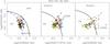 |
Fig. 2 e) As Fig. 2a but for MCG +02-20-003. |
| In the text | |
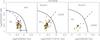 |
Fig. 2 f) As Fig. 2a but for NGC 5936. |
| In the text | |
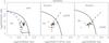 |
Fig. 2 g) As Fig. 2a but for NGC 6701. |
| In the text | |
|
Fig. 2 h) As Fig. 2a but for NGC 7469. The Hβ and Hα measurements correspond to the narrow component of the lines (see Paper I for details). |
| In the text | |
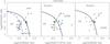 |
Fig. 2 i) As Fig. 2a but for NGC 7591. |
| In the text | |
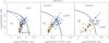 |
Fig. 2 j) As Fig. 2a but for NGC 7771. |
| In the text | |
Current usage metrics show cumulative count of Article Views (full-text article views including HTML views, PDF and ePub downloads, according to the available data) and Abstracts Views on Vision4Press platform.
Data correspond to usage on the plateform after 2015. The current usage metrics is available 48-96 hours after online publication and is updated daily on week days.
Initial download of the metrics may take a while.