© ESO, 2010

1. Introduction

Active galactic nuclei (AGN) consist of an accreting supermassive black hole (SMBH) in the center of a galaxy and sometimes exhibit powerful radio-emitting jets (Begelman et al. 1984). Radio-loud AGNs have continuum emission along the whole electromagnetic spectrum, from radio to gamma rays (e.g. Boettcher 2007). This radiation basically comes from the accretion disc and bipolar relativistic jets that originate close to the central SMBH. Radiation of accretion origin can be produced by the thermal plasma of either an optically-thick geometrically-thin disc under efficient cooling (Shakura & Sunyaev 1973), or an optically-thin geometrically-thick corona (e.g. Liang & Thompson 1979). The emission from the jets is non-thermal and generated by a population of relativistic particles very likely accelerated in strong shocks, although other mechanisms are also possible (Rieger et al. 2007). This non-thermal emission is assumed to be produced by synchrotron and inverse Compton (IC) processes (e.g., Ghisellini et al. 1985), although hadronic models have been also considered to explain gamma-ray detections (e.g. Mannheim 1993; Mücke & Protheroe 2001; Aharonian 2002).

In addition to continuum radiation, AGNs also exhibit optical and ultra-violet lines. Some of these lines are broad, emitted by gas moving with velocities v_g > 1000 km s^-1 and located in a small region close to the SMBH, the so-called broad line region (BLR). The structure of this region is not well known, but some models assume that the material in the BLR may have been formed by dense clouds confined within a hot (T ~ 10⁸ K) external medium (Krolik et al. 1981) or by magnetic fields (Rees 1987). These clouds would be ionized by photons from the accretion disc producing the observed emission lines, which are broad because of the cloud motion within the SMBH potential well. An alternative model proposes that the broad lines are produced in the chromosphere of evolved stars (Penston 1988) present in the nuclear region of AGNs.

The presence of material surrounding the base of the jets in AGNs makes jet-medium interactions very likely. For instance, the interaction of BLR clouds with a jet in AGNs was already suggested by Blandford & Königl (1979) as a mechanism for knot formation in the radio galaxy M87. Gamma-ray production by the interaction of a cloud from the BLR with a proton beam or a massive star with a jet were studied in the context of AGNs by Dar & Laor (1997) and Bednarek & Protheroe (1997), respectively.

In this work, we study the interaction of BLR clouds with the innermost jet in an AGN and its observable consequences at high energies. The approach adopted is similar to that followed in Araudo et al. (2009) for high-mass microquasars (for a general comparison between these sources and AGNs see Bosch-Ramon 2008), where the interaction of stellar wind clumps of the companion star with the microquasar jet was studied. In magnetic fields below equipartition with the jet kinetic energy (i.e. where the jet should be matter dominated), cloud penetration will lead to the formation of a relativistic bow shock in the jet and a slow shock inside the cloud. Electrons and protons can be efficiently accelerated in the bow shock and produce non-thermal emission, in situ by means of synchrotron and synchrotron self-Compton (SSC) mechanisms, and in the cloud through proton-proton (pp) collisions. For magnetic fields well below equipartition, the SSC component becomes the dominant electron-cooling channel, leading to significant gamma-ray production. Since the bow shock downstream is almost at rest in the laboratory reference frame (RF), this emission will not be boosted significantly. The resulting spectrum and the achieved luminosities in one jet-cloud interaction depend strongly on the magnetic field, the location of the interaction region, the cloud size, and the jet luminosity. However, many clouds may be inside the jet simultaneously, and the BLR global properties, such as size and total number of clouds, would also be relevant. Depending on whether one cloud or many of them penetrate into the jet, the light curve will be flare-like or rather steady, respectively.

To explore the radiative outcomes of jet-cloud interactions in AGNs, we apply our model to both Faranoff-Riley galaxies I (FR I) and II (FR II). In particular, we consider Centaurus A (Cen A) and 3C 273, the nearest FR I and a close and very bright flat spectrum radio quasar (with FR II as parent population), respectively, as illustrative cases. Although in FR I the BLR is not well-detected, clouds with similar characteristics to those found in FR II galaxies may surround the SMBH (Wang et al. 1986; Risaliti 2010). Cen A has been detected at high- (HE) (Hartman et al. 1999; Abdo et al. 2010) and very high-energy (VHE) gamma rays (Aharonian et al. 2009), whereas 3C 273 has been detected so far only at HE gamma rays (Hartman et al. 1999; Abdo et al. 2010). We computed the contribution of jet-cloud interactions to the gamma-ray emission in these sources, and estimated the gamma-ray luminosity in a wide range of cases. We found that gamma rays from jet-cloud interactions should be detectable by present and future instrumentation in nearby low-luminous AGNs at HE and VHE, and in powerful and nearby quasars only at HE because the VHE radiation is absorbed by the dense nuclear photon fields. In the case of sources exhibiting boosted gamma rays (blazars), the isotropic radiation from jet-cloud interactions will be masked by the jet beamed emission, which will not be the case in non-blazar sources.

The paper is organized as follows: in Sect. 2, the dynamics of jet-cloud interactions is described; in Sect. 3, a model for particle acceleration and emission is presented for one interaction, whereas in Sect. 4 the case of many clouds interacting with the jet is considered; in Sects. 5 and 6, the model is applied to FR I and FR II galaxies, focusing on the sources Cen A and 3C 273; finally, in Sect. 7, the results of this work are summarized and discussed. We adopt cgs units throughout this paper.

2. The jet-cloud interaction

For certain combinations of jet ram pressure, and cloud size and density, cloud-jet penetration is expected to occur. The details of the penetration process itself are complex. Here we do not treat them in detail, but just assume that penetration occurs if certain conditions are fulfilled. For low magnetic fields, a cloud inside the jet may represent a hydrodynamic situation in which a supersonic flow interacts with a body of approximately spherical shape at rest. The cloud, as long as it has not been accelerated by the jet ram pressure up to the jet speed (v_j), produces a perturbation in the jet medium in the form of a steady bow shock roughly at rest in the laboratory RF, moving at a velocity with respect to the jet RF approximately equal to v_j. Since the cloud is not rigid, a wave propagates also through it. Since the cloud temperature is much lower, and the density much higher than in the jet, this wave will be supersonic but much slower than the bow shock. The jet pressure exerts a force on the cloud leading to cloud acceleration along the axis, hydrodynamical instabilites, and, eventually, cloud fragmentation. In the following, the jet-cloud interaction is described. Further discussion, and a proper account of the literature, can be found in Araudo et al. (2009). Sketchs of the jet-cloud interaction and the jet-BLR scenario are shown in Fig. 1.

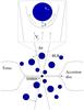Fig. 1 Sketch, not to scale, of an AGN on the spatial scales of the BLR region. In the top part of the figure, the interaction between a cloud and the jet is also shown.

We adopt here clouds with typical density n_c = 10¹⁰ cm^-3 and size R_c = 10¹³ cm (Risaliti 2010). The velocity of the cloud is taken v_c = 10⁹ cm s^-1 (Peterson 2006). The jet Lorentz factor is fixed to Γ = 10, implying v_j ≈ c, with a half-opening angle φ ≈ 6°, i.e. the jet radius/height relation fixed to R_j = tan(φ)z = 0.1z. All these parameters are summarized in Table 1 and will not change in the paper; from them, the jet density n_j in the laboratoty RF can be estimated to be $\begin{array}{ccc}{\mathit{n}}_{\mathrm{j}}\mathrm{=}\frac{{\mathit{L}}_{\mathrm{j}}}{\mathrm{(}\mathrm{\Gamma }\mathrm{-}\mathrm{1}\mathrm{)}{\mathit{m}}_{\mathrm{p}}{\mathit{c}}^{\mathrm{3}}{\mathit{\sigma }}_{\mathrm{j}}}& \mathrm{\approx }& \mathrm{8}\mathrm{\times }{\mathrm{10}}^{\mathrm{4}}\left(\frac{{\mathit{L}}_{\mathrm{j}}}{{\mathrm{10}}^{\mathrm{44}}\mathrm{erg}{\mathrm{s}}^{-1}}\right)\\ & & \mathrm{\times }{\left(\frac{\mathrm{\Gamma }\mathrm{-}\mathrm{1}}{\mathrm{9}}\right)}^{-1}{\left(\frac{\mathit{z}}{{\mathrm{10}}^{\mathrm{16}}\mathrm{cm}}\right)}^{-2}\mathrm{c}{\mathrm{m}}^{-3}\mathit{,}\end{array}$(1)where and L_j is the kinetic power of the matter-dominated jet.

The jet ram pressure should not destroy the cloud before it has fully entered into the jet. This means that the time required by the cloud to penetrate into the jet should be 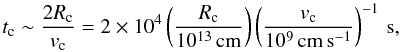${\mathit{t}}_{\mathrm{c}}\mathrm{~}\frac{\mathrm{2}{\mathit{R}}_{\mathrm{c}}}{{\mathit{v}}_{\mathrm{c}}}\mathrm{=}\mathrm{2}\mathrm{\times }{\mathrm{10}}^{\mathrm{4}}\left(\frac{{\mathit{R}}_{\mathrm{c}}}{{\mathrm{10}}^{\mathrm{13}}\mathrm{cm}}\right){\left(\frac{{\mathit{v}}_{\mathrm{c}}}{{\mathrm{10}}^{\mathrm{9}}\mathrm{cm}{\mathrm{s}}^{-1}}\right)}^{-1}\mathrm{s}\mathit{,}$(2)which in turn should be shorter than the cloud lifetime inside the jet. To estimate this cloud lifetime, we first compute the time required by the shock in the cloud to cross it (t_cs). The velocity of this shock, v_cs, can be derived by ensuring that the jet and the cloud shock ram pressures are equal, i.e., 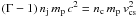, is valid as long as v_cs ≪ c. Then $\begin{array}{ccc}{\mathit{v}}_{\mathrm{cs}}\mathrm{~}{\mathit{\chi }}^{\mathrm{-}\mathrm{1}\mathit{/}\mathrm{2}}\mathit{c}& \mathrm{~}& \mathrm{3}\mathrm{\times }{\mathrm{10}}^{\mathrm{8}}{\left(\frac{{\mathit{n}}_{\mathrm{c}}}{{\mathrm{10}}^{\mathrm{10}}\mathrm{c}{\mathrm{m}}^{-3}}\right)}^{\mathrm{-}\mathrm{1}\mathit{/}\mathrm{2}}\\ & & \mathrm{\times }{\left(\frac{\mathit{z}}{{\mathrm{10}}^{\mathrm{16}}\mathrm{cm}}\right)}^{-1}{\left(\frac{{\mathit{L}}_{\mathrm{j}}}{{\mathrm{10}}^{\mathrm{44}}\mathrm{erg}{\mathrm{s}}^{-1}}\right)}^{\mathrm{1}\mathit{/}\mathrm{2}}\mathrm{cm}{\mathrm{s}}^{-1}\mathit{,}\end{array}$(3)where χ is the cloud to jet density ratio, n_c / n_j(Γ − 1). This yields a cloud shocking time of $\begin{array}{ccc}{\mathit{t}}_{\mathrm{cs}}\mathrm{~}\frac{\mathrm{2}{\mathit{R}}_{\mathrm{c}}}{{\mathit{v}}_{\mathrm{cs}}}& \mathrm{\simeq }& \mathrm{7}\mathrm{\times }{\mathrm{10}}^{\mathrm{4}}\left(\frac{{\mathit{R}}_{\mathrm{c}}}{{\mathrm{10}}^{\mathrm{13}}\mathrm{cm}}\right){\left(\frac{{\mathit{n}}_{\mathrm{c}}}{{\mathrm{10}}^{\mathrm{10}}\mathrm{c}{\mathrm{m}}^{-3}}\right)}^{\mathrm{1}\mathit{/}\mathrm{2}}\\ & & \mathrm{\times }\left(\frac{\mathit{z}}{{\mathrm{10}}^{\mathrm{16}}\mathrm{cm}}\right){\left(\frac{{\mathit{L}}_{\mathrm{j}}}{{\mathrm{10}}^{\mathrm{44}}\mathrm{erg}{\mathrm{s}}^{-1}}\right)}^{\mathrm{-}\mathrm{1}\mathit{/}\mathrm{2}}\mathrm{s}\mathit{.}\end{array}$(4)Therefore, for a penetration time (t_c) at least as short as  ~t_cs, the cloud will remain an effective obstacle for the jet flow. Setting t_c ~ t_cs, we obtain a minimum value for χ and hence for z.

Hydrodynamical instabilities produced by the interaction with the jet material affect the cloud. First of all, the jet exerts a force on the cloud through the contact discontinuity. The acceleration applied to the cloud can be estimated from the jet ram pressure P_j, and the cloud section and mass $\mathit{g}\mathrm{=}\frac{{\mathit{P}}_{\mathrm{j}}{\mathit{\sigma }}_{\mathrm{c}}}{{\mathit{M}}_{\mathrm{c}}}\mathrm{~}\frac{\mathrm{3}}{\mathrm{4}}\frac{{\mathit{c}}^{\mathrm{2}}}{\mathit{\chi }{\mathit{R}}_{\mathrm{c}}}\mathrm{=}\frac{\mathrm{3}}{\mathrm{2}}\frac{{\mathit{v}}_{\mathrm{cs}}}{{\mathit{t}}_{\mathrm{cs}}}\mathrm{·}$(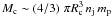5)Given the acceleration exerted by the jet in the cloud, Rayleigh-Taylor (RT) instabilities will develop in the cloud, at the jet contact discontinuity, on a timescale ${\mathit{t}}_{\mathrm{RT}}\mathrm{~}\sqrt{\frac{\mathit{l}}{\mathit{g}}}\mathrm{=}\sqrt{\frac{\mathrm{4}\mathit{\chi l}{\mathit{R}}_{\mathrm{c}}}{\mathrm{3}{\mathit{c}}^{\mathrm{2}}}}\mathit{,}$(6)where the instability length l is the spatial scale of the perturbation. For perturbations in the size of the cloud l ~ R_c associated with cloud significant disruption, one finds that t_RT ~ t_cs.

In addition to RT instabilities, Kelvin-Helmholtz (KH) instabilities also grow within the cloud walls in contact with the shocked jet material surrounding the cloud. Accounting for the high relative velocity, v_rel ≲ v_j, one obtains ${\mathit{t}}_{\mathrm{KH}}\gtrsim \sqrt{\frac{\mathit{l}}{{\mathit{g}}_{\mathrm{rel}}}}\mathrm{=}\frac{\mathit{\chi l}}{\mathit{c}}\mathit{,}$(7)where g_rel ~ c² / χl. For l ~ R_c, we obtain t_KH ≳ t_cs. In the previous estimates of t_RT and t_KH, we did not take into account the effect of the magnetic field (e.g. Blake 1972), since we assume that it is dynamically negligible. We note that, given g, the time to accelerate the cloud to the shock velocity v_cs is  ~ t_cs. However, the timescale to accelerate the cloud to v_j is  ≫ t_cs provided that v_j ≫ v_cs, and before this occurs, the cloud will likely fragment.

Finally, two additional timescales are relevant to our study, the bow-shock formation time, t_bs, and the time required by the cloud to cross the jet, t_j. The timescale t_bs can be roughly estimated assuming that the shock downstream has a cylindrical shape with one of the bases being the bow shock, relativistic shock jump conditions, equal particle injection and escape rates, and a escape velocity similar to the sound speed (for a relativistic plasma). This yields a shock-cloud separation distance of Z ~ 0.3R_c, which implies that ${\mathit{t}}_{\mathrm{bs}}\mathrm{~}\frac{\mathit{Z}}{\mathit{c}}\mathrm{=}{\mathrm{10}}^{\mathrm{2}}\left(\frac{{\mathit{R}}_{\mathrm{c}}}{{\mathrm{10}}^{\mathrm{13}}\mathrm{cm}}\right)\mathrm{s}\mathit{.}$(8)Since in general t_bs ≪ t_cs, we can assume that the bow shock is in the steady regime. The jet crossing time t_j can be characterized by ${\mathit{t}}_{\mathrm{j}}\mathrm{~}\frac{\mathrm{2}{\mathit{R}}_{\mathrm{j}}}{{\mathit{v}}_{\mathrm{c}}}\mathrm{=}\mathrm{2}\mathrm{\times }{\mathrm{10}}^{\mathrm{6}}\left(\frac{\mathit{z}}{{\mathrm{10}}^{\mathrm{16}}\mathrm{cm}}\right){\left(\frac{{\mathit{v}}_{\mathrm{c}}}{{\mathrm{10}}^{\mathrm{9}}\mathrm{cm}{\mathrm{s}}^{-1}}\right)}^{-1}\mathrm{s}\mathit{.}$(9)We note that if the cloud lifetime is  < t_j, the number of clouds inside the jet will be smaller than expected from the BLR properties alone.

To summarize the dynamics of the jet-cloud interaction, we plot in Fig. 2 the t_cs (for different L_j), t_j, t_c, and t_bs as a function of z. As shown in the figure, for some values of z and L_j the cloud may be destroyed by the jet before full penetration, i.e. t_cs < t_c. This is a constraint to determine the height z of the jet at which the cloud can penetrate into it. We also note that, in general, t_bs is much shorter than any other timescale.

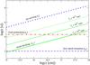Fig. 2 The jet crossing (blue dotted line), cloud penetration (red dot-dashed line), bow-shock formation (violet dashed line), and cloud shocking (green solid lines) times are plotted; all of them have been calculated using the values given in Table 1. The time tcs is plotted for Lj = 1044, 1046, and 1048 erg s-1.

2.1. The interaction height

The cloud can fully penetrate into the jet if the cloud lifetime after jet impact is longer than the penetration time (the weaker condition that jet lateral pressure is is then automatically satisfied). This determines the minimum interaction height, z_int, to avoid cloud disruption before full penetration. This interaction also, cannot occur within the jet formation region, z₀ ~ 100R_g ≈ 1.5 × 10¹⁵(M_bh / 10⁸M_⊙) cm (Junor et al. 1999). For BLR-jet interaction and cloud penetration to occur, the size of the BLR should be R_blr > z₀ and z_int.

The lifetime of the cloud depends on the fragmentation time, which is strongly linked to, but longer than, t_cs. The value of z_int can then be estimated by setting t_c ≲ t_cs, since the cloud should enter the jet before being significantly distorted by the impact of the latter. Once shocked, the cloud may suffer lateral expansion and conduction heating, which can speed up fragmentation due to instabilities. In this work, we choose z_int fixing t_cs = 2t_c$\begin{array}{ccc}{\mathit{z}}_{\mathrm{int}}& \mathrm{\approx }& \mathrm{5}\mathrm{\times }{\mathrm{10}}^{\mathrm{15}}{\left(\frac{{\mathit{v}}_{\mathrm{c}}}{{\mathrm{10}}^{\mathrm{9}}\mathrm{cm}{\mathrm{s}}^{-1}}\right)}^{-1}{\left(\frac{{\mathit{n}}_{\mathrm{c}}}{{\mathrm{10}}^{\mathrm{10}}\mathrm{c}{\mathrm{m}}^{-3}}\right)}^{\mathrm{-}\mathrm{1}\mathit{/}\mathrm{2}}\\ & & \mathrm{\times }{\left(\frac{{\mathit{L}}_{\mathrm{j}}}{{\mathrm{10}}^{\mathrm{44}}\mathrm{erg}{\mathrm{s}}^{-1}}\right)}^{\mathrm{1}\mathit{/}\mathrm{2}}\mathrm{cm}\mathit{.}\end{array}$(10)We note that the available power in the bow shock is L_bs ~ (σ_c / σ_j)L_j ∝ z^-2. Therefore, the most luminous individual jet-cloud interaction will take place at z ~ z_int.

The BLR size can be estimated using an empirical relation derived for sources with a well-established BLR, i.e. FR II radio galaxies. This relation is in general of type , where L_blr is the luminosity of the BLR and α ~ 0.5 − 0.7 (e.g. Kaspi et al. 2005, 2007; Peterson et al. 2005; Bentz et al. 2006). In this paper, we use the relations ${\mathit{R}}_{\mathrm{blr}}\mathrm{~}\mathrm{6}\mathrm{\times }{\mathrm{10}}^{\mathrm{16}}{\left(\frac{{\mathit{L}}_{\mathrm{blr}}}{{\mathrm{10}}^{\mathrm{44}}\mathrm{erg}{\mathrm{s}}^{-1}}\right)}^{\mathrm{0.7}}\mathrm{cm}\mathit{,}$(11)and ${\mathit{R}}_{\mathrm{blr}}\mathrm{~}\mathrm{2.5}\mathrm{\times }{\mathrm{10}}^{\mathrm{16}}{\left(\frac{{\mathit{L}}_{\mathrm{blr}}}{{\mathrm{10}}^{\mathrm{44}}\mathrm{erg}{\mathrm{s}}^{-1}}\right)}^{\mathrm{0.55}}\mathrm{cm}\mathit{,}$(12)from Kaspi et al. (2005, 2007).

In Fig. 3, we show the relation of z_int and R_blr with L_j, assuming that L_blr is 10% of the disc luminosity, which is assumed here to equal L_j. As seen in the figure, for reasonable parameters, the condition z_int < R_blr is fulfilled for a wide range of L_j. Figure 3 also shows the relation between z₀ and M_bh, which shows that for M_bh ≳ 10⁹ M_⊙ the jet may not even be (fully) formed at the BLR scales at the lowest L_j-values.

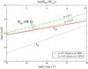Fig. 3 The interaction height, zint (red solid line), and the size of the BLR, Rblr (green dashed line), for different values of Lj (bottom horizontal axis). We have derived Rblr(Lj) fixing Lblr = 0.1Lj and plotted Rblr using Eqs. (11) and (12). In the same plot, the height of the jet base, z0 (blue dotted line), is plotted as a function of MBH (top horizontal axis).

3. Non-thermal particles and their emission

In the bow and cloud shocks, particles can be accelerated by means of diffusive shock acceleration (Bell 1978). However, the bow shock should be more efficient in accelerating particles than the shock in the cloud because v_bs ≫ v_cs. In addition, the cloud shock luminosity is lower than the bow-shock luminosity by  ~ 1 / (2χ^1 / 2). For these reasons, we focus here on the particle acceleration in the bow shock. In this section, we briefly describe the injection and evolution of particles, and their emission, highlighting aspects that are specific to AGNs. The details of the emitting processes considered here (synchrotron, IC, and pp interactions) can be found in Araudo et al. (2009) and references therein.

First, one can estimate the non-thermal luminosity, L_nt, injected at z_int in the bow shock in the form of relativistic electrons or protons $\begin{array}{ccc}{\mathit{L}}_{\mathrm{nt}}\mathrm{=}{\mathit{\eta }}_{\mathrm{nt}}{\mathit{L}}_{\mathrm{bs}}& \mathrm{\approx }& \mathrm{4}\mathrm{\times }{\mathrm{10}}^{\mathrm{39}}\left(\frac{{\mathit{\eta }}_{\mathrm{nt}}}{\mathrm{0.1}}\right){\left(\frac{{\mathit{R}}_{\mathrm{c}}}{{\mathrm{10}}^{\mathrm{13}} \mathrm{cm}}\right)}^{\mathrm{2}}\\ & & \mathrm{\times }\left(\frac{{\mathit{L}}_{\mathrm{j}}}{{\mathrm{10}}^{\mathrm{44}}\mathrm{erg}{\mathrm{s}}^{-1}}\right)\mathrm{erg}{\mathrm{s}}^{-1}\mathit{.}\end{array}$(13)The accelerator/emitter magnetic field in the bow-shock RF (B) can then, be determined by relating U_B = η_BU_nt, where U_B = B² / 8π and U_nt = L_nt / (σ_cc) are the magnetic and the non-thermal energy densities, respectively. For leptonic emission and to avoid supression of the IC channel, high gamma-ray outputs require η_B well below 1. 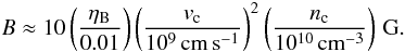In this context, B can be parametrized to be $\mathit{B}\mathrm{\approx }\mathrm{10}\left(\frac{{\mathit{\eta }}_{\mathrm{B}}}{\mathrm{0.01}}\right){\left(\frac{{\mathit{v}}_{\mathrm{c}}}{{\mathrm{10}}^{\mathrm{9}}\mathrm{cm}{\mathrm{s}}^{-1}}\right)}^{\mathrm{2}}\left(\frac{{\mathit{n}}_{\mathrm{c}}}{{\mathrm{10}}^{\mathrm{10}}\mathrm{c}{\mathrm{m}}^{-3}}\right)\mathrm{G}\mathit{.}$(14)Regarding the acceleration mechanism, since the bow shock is relativistic and the treatment of these shocks is complex (see Achterberg et al. 2001), we adopt a prescription for the acceleration rate of $\mathit{Ė}\mathrm{acc}\mathrm{=}\mathrm{0.1}\mathit{qBc,}$(15)similar to that in the relativistic termination shock of the Crab pulsar wind (de Jager et al. 1996).

Particles are affected by different losses that balance the energy gain from acceleration. The electron loss mechanisms include escape downstream, relativistic bremsstrahlung, synchrotron emission, and external Compton (EC) and SSC. We note that B, L_nt, and the accelerator/emitter size at z_int are constant for different L_j and fixed η_B and η_nt, and only L_blr and L_d are expected to change with L_j. Therefore, as long as the external photon fields are negligible, the maximum electron energy at z_int does not change for different jet powers.

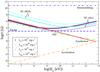Fig. 4 Acceleration gain (orange dot-dashed line), escape (blue dashed line), and cooling lepton timescales are plotted. SSC (green two-dot-dashed line) is plotted when the steady state is reached and EC for the both BLR (turquoise square line) and disc (maroon dotted line) photon fields are shown for the conditions of faint (BLR: 1044; disc: 1045 erg s-1) and bright sources (BLR: 1046; disc: 1047 erg s-1). Synchrotron (red solid line) and relativistic bremsstrahlung (violet dot-two-dashed line) are also plotted. We have fixed ηB = 0.01. For protons, the pp cooling timescale is not shown for clarity, although it is similar to that of relativistic bremsstrahlung.

In Fig. 4, the leptonic cooling timescales are plotted with the escape time and the acceleration time for a bow shock located at z_int. A value of η_B equal to 0.01 has been adopted. The SSC cooling timescale is plotted for the steady state. The escape time downstream from the relativistic bow shock is taken to be ${\mathit{t}}_{\mathrm{esc}}\mathrm{~}\frac{\mathrm{3}{\mathit{R}}_{\mathrm{c}}}{\mathit{c}}\mathrm{=}{\mathrm{10}}^{\mathrm{3}}\left(\frac{{\mathit{R}}_{\mathrm{c}}}{{\mathrm{10}}^{\mathrm{13}}\mathrm{cm}}\right)\mathrm{s}\mathit{.}$(16)Synchrotron and EC/SSC are the dominant processes in the high-energy part of the electron population, relativistic bremsstrahlung is negligible for any energy, and electron escape is relevant in the low-energy part. This yields a break in the electron energy distribution at the energy for which the synchrotron/IC time and the escape time are equal. The Thomson to KN transition is clearly seen in the EC cooling curves, but is much smoother in the SSC case. The maximun electrons energy are around several TeV. Given the similar cooling timescale for electrons by means of relativistic bremsstrahlung and protons by pp collisions (t_brems / pp ~ 10¹⁵ / n s, where n is the target density), protons will not cool efficiently in the bow shock. Photomeson production can also be discarded as a relevant proton cooling mechanism in the bow shock due to the relatively low achievable proton energies and photon densities. The maximum energy of protons is constrained by equating the acceleration time and the time needed to diffuse out of the bow shock. Assuming Bohm diffusion, t_diff = 3Z² / 2r_gc (where r_g is the particle gyroradius), the maximum proton energy is ${\mathit{E}}_{\mathrm{p}}^{\max }\mathrm{~}\mathrm{0.1}\mathit{qB}{\mathit{R}}_{\mathrm{c}}\mathrm{=}\mathrm{5}\mathrm{\times }{\mathrm{10}}^{\mathrm{3}}\left(\frac{\mathit{B}}{\mathrm{10}\mathrm{G}}\right)\left(\frac{{\mathit{R}}_{\mathrm{c}}}{{\mathrm{10}}^{\mathrm{13}}\mathrm{cm}}\right)\mathrm{TeV}\mathit{.}$(17)Electrons and protons are injected into the bow shock region following a power law in energy of index 2.2 (Achterberg et al. 2001) with an exponential cutoff at the maximum electron/proton energy. The injection luminosity is L_nt.

To first order, the electron evolution can be computed assuming homogeneous conditions, following therefore a one-zone approximation with all the mentioned cooling and escape processes. The formulae for all the relevant radiative mechanisms, as well as the solved electron evolution differential equation, can be found in Araudo et al. (2009). In some cases, SSC is the dominant cooling channel at high energies. In that case, the calculations have to be performed numerically by separating the evolution of the electron population into different time steps. In each step, the radiation field is updated by accounting for the synchrotron emission produced in the previous step until the steady state is reached. The duration of each step should be shorter for the earlier phases of the evolutionary state to account properly for the rise in the synchrotron energy density of the emitter.

Once the steady-state electron distribution in the bow shock is computed, the spectral energy distribution (SED) of the non-thermal radiation can be calculated. The synchrotron self-absorption effect has to be taken into account, which will affect the low energy band of the synchrotron emission. At gamma-ray energies, photon-photon absorption due to the disc and the BLR radiation should be considered, the internal absorption due to synchrotron radiation being negligible. Given the typical BLR and disc photon energies,  ~ 10 eV and  ~ 1 keV, respectively, gamma rays beyond 1 GeV and 100 GeV can be strongly affected by photon-photon absorption. On the other hand, in most cases photons of energies between 100 MeV and 1 GeV will escape the dense disc photon field.

Although proton cooling is negligible in the bow-shock region, it may be significant in the cloud. Protons can penetrate into the cloud if t_esc > t_diff, which yields a minimum energy to reach the cloud of . These protons will radiate in the form of gamma rays only a fraction  ~ 3 × 10^-4(R_c / 10¹³cm)(t_pp / 10⁵s)^-1 of their energy, implying that the process is rather inefficient. The reason is that these protons cannot be efficiently confined and cross the cloud at a velocity  ~ c. For further details of the proton energy distribution in the cloud, we refer to Araudo et al. (2009).

4. Many clouds inside the jet

Clouds fill the BLR, and many of them may be simultaneously inside the jet at different z, each of them producing non-thermal radiation. Therefore, the total luminosity may be much larger than that produced by just one interaction, which is  ~ L_nt. The number of clouds within the jets, at z ≤ R_blr, can be computed from the jet (V_j) and cloud (V_c) volumes, resulting in ${\mathit{N}}_{\mathrm{c}}^{\mathrm{j}}\mathrm{=}\mathrm{2}\mathit{f}\frac{{\mathit{V}}_{\mathrm{j}}}{{\mathit{V}}_{\mathrm{c}}}\mathrm{~}\mathrm{9}{\left(\frac{{\mathit{L}}_{\mathrm{j}}}{{\mathrm{10}}^{\mathrm{44}}\mathrm{erg} {\mathrm{s}}^{-1}}\right)}^{\mathrm{2}}{\left(\frac{{\mathit{R}}_{\mathrm{c}}}{{\mathrm{10}}^{\mathrm{13}}\mathrm{cm}}\right)}^{-3}\mathit{,}$(18)where the factor 2 accounts for the two jets and f ~ 10^-6 is the filling factor of clouds in the whole BLR (Dietrich et al. 1999). In reality, is correct if one neglects that the cloud disrupts and fragments, and eventually dilutes inside the jet. For instance, Klein et al. (1994) estimated a shocked cloud lifetime of several t_cs, and Shin et al. (2008) found that even a weak magnetic field in the cloud can significantly increase its lifetime. Finally, even under cloud fragmentation, strong bow shocks can form around the cloud fragments before these have accelerated close to v_j. All this makes the real number of interacting clouds inside the jet difficult to estimate, but it should be between and .

The presence of many clouds inside the jet, not only at z_int but also at higher z, implies that the total non-thermal luminosity available in the BLR-jet intersection region is $\begin{array}{ccc}{\mathit{L}}_{\mathrm{nt}}^{\mathrm{tot}}& \mathrm{~}& \mathrm{2}{\mathrm{\int }}^{{\mathit{R}}_{\mathrm{blr}}}\frac{\mathrm{d}{\mathit{N}}_{\mathrm{c}}^{\mathrm{j}}}{\mathrm{d}\mathit{z}}{\mathit{L}}_{\mathrm{nt}}\mathrm{\left(}\mathit{z}\mathrm{\right)}\mathrm{d}\mathit{z}\\ & \mathrm{~}& \mathrm{2}\mathrm{\times }{\mathrm{10}}^{\mathrm{40}}\left(\frac{{\mathit{\eta }}_{\mathrm{nt}}}{\mathrm{0.1}}\right){\left(\frac{{\mathit{R}}_{\mathrm{c}}}{{\mathrm{10}}^{\mathrm{13}}\mathrm{cm}}\right)}^{-1}{\left(\frac{{\mathit{L}}_{\mathrm{j}}}{{\mathrm{10}}^{\mathrm{44}}\mathrm{erg}{\mathrm{s}}^{-1}}\right)}^{\mathrm{1.7}}\mathit{,}\end{array}$(19)where is the number of clouds located in a jet volume dV_j = π(0.1z)²dz. In both Eqs. (18) and (19), L_blr has been fixed to 0.1L_j, as approximately found in FR II galaxies, and R_blr has been derived using Eq. (11).

In Fig. 5, we show estimates of the gamma-ray luminosity when many clouds interact simultanously with the jet. For this, we have followed a simple approach assuming that most of the non-thermal luminosity is converted into gamma rays. This will be the case as long as the escape and synchrotron cooling time are longer than the IC cooling time (EC+SSC) at the highest electron energies. Given the little information about the BLR available for FR I sources, we do not specifically consider these sources here.

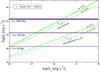Fig. 5 Upper limits to the gamma-ray luminosity produced by clouds inside the jet as a function of Lj in FR II sources. Two cases are plotted, one assuming that clouds cross the jet without disruption (green solid lines), and one in which the clouds are destroyed in a time as short as tcs (green dashed lines). The thick (solid and dashed) and thin (solid and dashed) lines correspond to (Kaspi et al. 2007) and (Kaspi et al. 2005), respectively. In addition, the sensitivity levels of Fermi in the range 0.1–1 GeV (maroon dotted lines) are plotted for three different distances d = 10, 100, and 1000 Mpc.

In the next two sections, we present more detailed calculations by applying the model presented in Sect. 3 to two characteristic sources, Cen A (FR I, one interaction) and 3C 273 (FR II, many interactions).

5. Application to FR I galaxies: Cen A

At a distance d ≈ 3.7 Mpc, Cen A is the closest AGN (Israel 1998). It has been classified as both an FR I radio galaxy and a Seyfert 2 optical object. The mass of the black hole is  ≈6 × 10⁷ M_⊙ (Marconi et al. 2000). The angle between the jets and the line of sight is large  >50° (Tingay et al. 1998), thus the jet radiation towards the observer should not experience strong beaming. The jets of Cen A are disrupted on kpc scales, forming two giant radio lobes that extend  ~10° across the southern sky. At optical wavelenghts, the nuclear region of Cen A is obscured by a dense region of gas and dust, probably as a consequence of a recent merger (Thomson 1992; Mirabel et al. 1999). At higher energies, Chandra and XMM-Newton detected continuum X-ray emission originating in from the nuclear region, with a luminosity  ~5 × 10⁴¹ erg s^-1 at energies of 2–7 keV (Evans et al. 2004). These X-rays could be produced by the accretion flow and the inner jet, although their origin remains unclear. In the GeV range, Cen A was detected above 200 MeV by Fermi, with a bolometric luminosity of  ≈ 4 × 10⁴⁰ erg s^-1 (Abdo et al. 2009), and above  ~200 GeV by HESS, with a bolometric luminosity of  ≈ 3 × 10³⁹ erg s^-1 (Aharonian et al. 2009). In both cases, this HE emission is associated with the nuclear region. Cen A has been proposed to be a source of ultra HE cosmic rays (Romero et al. 1996).

A BLR has not yet been detected in Cen A (Alexander et al. 1999), although this may be a consequence of the optical obscuration produced by the dust lane. One can still assume that clouds surround the SMBH in the nuclear region (Wang et al. 1986; Risaliti et al. 2002) but, because of the low luminosities of the accretion disc, it is not expected that the photoionization of these clouds will be efficient enough to produce lines. Since no emission from these clouds is assumed, we only consider the EC scattering with photons from the accretion flow.

We adopt here a jet power for Cen A of L_j = 10⁴⁴ erg s^-1. From this value, and the values given in Sect. 2 for the remaining parameters of the jet and the cloud, z_int results in  ≈ 5 × 10¹⁵ cm. At this jet height, the emission produced by the interaction between one cloud and the jet is calculated assuming a η_B = 0.01, and the corresponding SED is presented in Fig. 6. As mentioned in Sect. 3, the low-energy band of the synchrotron spectrum is self-absorbed at energies below  ~ 10^-4 eV. At gamma-ray energies, photon-photon absorption is negligible due to the weak ambient photon fields (e.g. Rieger & Aharonian 2009; Araudo et al. 2009, 2010a,b). At high energies, SSC dominates the radiative output, with the computed luminosity above 100 MeV being  ~ 2 × 10³⁹ erg s^-1, and above 100 GeV about 10 times less. These luminosities are below the sensitivity of Fermi and HESS and one order of magnitude lower than the observed ones. We note however that , and for slightly larger clouds, L_nt may increase to detectable levels. The penetration of a large clump into the base of the jet of Cen A would lead to a flare with a duration of about one day.

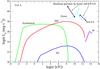Fig. 6 Computed SED for one jet-cloud interaction at zint in Cen A. We also show the SEDs of the detected emission by Fermi and HESS, as well as the sensitivity curves of these instruments.

6. Application to FR II galaxies: 3C 273 (off-axis)

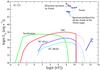Fig. 7 Computed SED for one jet-cloud interaction at zint in 3C 273. The emission in the 0.1–1 GeV range from many clouds inside the jet is also shown, together with the sensitivity level of Fermi and the observed SED above 200 MeV.

At a distance of d = 6.7 × 10² Mpc, 3C 273 is a powerful radio-loud AGN (Courvoisier 1998) with a SMBH mass M_BH ~ 7 × 10⁹   M_⊙ (Paltani & Türler 2005). The angle of the jet to the line of sight is small,  ≈ 6°, which implies that 3C 273 is a blazar (Jolley et al. 2009). The whole spectrum of this source exhibits variability (e.g. Pian et al. 1999) from years (radio) to few hours (gamma rays). At high energies, 3C 273 was the first blazar AGN detected in the MeV band by the COS-B satellite and, later on, by EGRET (Hartman et al. 1999). This source was also detected at GeV energies by Fermi and AGILE, but has not yet been detected in the TeV range. Given the jet luminosity of 3C 273 of L_j ≈ 4 × 10⁴⁷ erg s^-1 (Kataoka et al. 2002), z_int found to be  ≈ 3 × 10¹⁷ cm. The BLR luminosity of this source is  ≈ 4 × 10⁴⁵ erg s^-1 (Cao & Jiang 1999), and its size 7 × 10¹⁷ cm (Ghisellini et al. 2010), which implies that jet-cloud interactions can take place. The disc luminosity is high,  ≈ 2 × 10⁴⁶ erg s^-1, for typical photon energies  ≈ 54 eV (Grandi & Palumbo 2004).

The non-thermal SED of the radiation generated by jet-cloud interactions in 3C 273 is shown in Fig. 7. At z_int, the most important radiative processes are synchroton and SSC. The bolometric luminosities generated by these processes in one interaction at z_int are 6 × 10³⁸ erg s^-1 and 2 × 10³⁹ erg s^-1, respectively. Given the strong radiation fields from the disc and the BLR, the emission above  ~ 10 GeV is absorbed by photon-photon absorption, and the maximum of the emission occurs around 0.1–1 GeV. Given the estimated number of clouds in the BLR of 3C 273,  ~ 10⁸ (Dietrich et al. 1999), and the size of R_blr ≈ 7 × 10¹⁷ cm, we find the filling factor to be f ~ 3 × 10^-7. With this value of f, the number of clouds in the two jets results in  ~ 2 × 10³ and 5 × 10⁵ for both the minimum and maximum values (see Sect. 4). In the most optimistic case, the SSC luminosity would reach 2 × 10⁴⁴ erg s^-1. This value is well below the observed luminosity by Fermi in the GeV range,  ~ 3 × 10⁴⁶ erg s^-1 in the steady state and  ~ 1.7 × 10⁴⁷ erg s^-1 in flares (Soldi et al. 2009). However, the detected emission is very likely of beamed origin and should mask any unbeamed radiation. However, powerful non-blazar AGNs (FR II galaxies) do not contain this beamed component, which makes it possible to detect GeV emission from jet-cloud interactions in these sources. In this case, given that many BLR clouds can interact with the jet simultaneously, the radiation should be steady.

7. Summary and discussion

We have studied the interaction of clouds with the base of jets in AGNs. Considering reasonable cloud and jet parameters, we have estimated the relevant dynamical timescales of these interactions, concluding that clouds can enter into the jet only above a certain height,  ~ z_int. Below z_int, the jet is too compact and its ram/magnetic pressure will destroy the cloud before fully penetrating into the jet. When the cloud interacts significantly with the jet, strong shocks are generated and gamma rays can be produced with an efficiency that depends strongly on the bow-shock magnetic field.

For very high B-values (Poynting-flux dominated jets), the treatment performed here does not apply. In that case, z_int could still be defined by adopting the jet magnetic pressure instead of the ram pressure. If a cloud entered into such a jet, particle acceleration in the bow shock could still occur due to, for instance, magnetic reconnection. A study of this case would require a completely different approach from the one presented here. In general, for bow-shock magnetic fields above equipartition with non-thermal particles, the IC channel and gamma ray production will be suppressed in favor of synchrotron emission, unless magnetic dissipation reduces the magnetic field sufficiently for IC to be dominant. Bow shock B-values well below equipartition with non-thermal particles produce significant gamma-ray emission. We note that the modeling of gamma rays from AGN jets uses to require relatively low magnetic fields (e.g. Ghisellini et al. 2010). Therefore, it may be that, even if the jet magnetic field were high at z_int, it could become small enough at greater heights thanks to bulk acceleration (e.g. Komissarov et al. 2007) or some other form of magnetic dissipation.

For very nearby sources, such as Cen A, the interaction of large clouds with jets may be detectable as a flaring event, although the number of these large clouds and thereby the duty cycle of the flares are difficult to estimate. Given the weak external photon fields in these sources, VHE photons can escape without experiencing significant absorption. Therefore, jet-cloud interactions in nearby FR I may be detectable in both the HE and the VHE range as flares with timescales of about one day. Studying this a radiation would provide information on the environmental conditions and the base of the jet in these sources.

In FR II sources, many BLR clouds may interact simultaneously with the jet. The number of clouds depends strongly on the cloud lifetime inside the jet, which could be of the order of several t_cs. Nevertheless, we note that after cloud fragmentation many bow shocks may still form and efficiently accelerate particles if these fragments move more slowly than the jet. Since FR II sources are expected to exhibit high accretion rates, radiation above 1 GeV produced in the jet base can be strongly attenuated by the dense disc and the BLR photon fields, although gamma rays below 1 GeV should not be affected significantly. Since jet-cloud emission should be rather isotropic, it would be masked by jet beamed emission in blazar sources, although since powerful/nearby FR II jets do not display significant beaming, these objects may emit gamma rays from jet-cloud interactions. In the context of AGN unification (Urry & Padovani 1995), the number of non-blazar (radio-loud) AGNs should be much larger than that of blazars with the same L_j. As shown in Fig. 5, close and powerful sources could be detectable by deep enough observations of Fermi. After few-year exposure times, a significant signal from these objects could be found, their detection providing strong evidence that jets are already strongly matter dominated at the bow shock regions, as well as physical information on the BLR and jet base region.

Acknowledgments

We thank the referee Elena Pian for constructive comments and sugestions. A.T.A. and V.B.-R. thanks Max Planck Institut fuer Kernphysik for kind hospitality and support. A.T.A. and G.E.R. are supported by CONICET and the Argentine agency ANPCyT (grant BID 1728/OC-AR PICT 2007-00848). V.B.-R. and G.E.R. acknowledge support by the Ministerio de Educación y Ciencia (Spain) under grant AYA 2007-68034-C03-01, FEDER fund

References

All Tables

All Figures

	Fig. 1 Sketch, not to scale, of an AGN on the spatial scales of the BLR region. In the top part of the figure, the interaction between a cloud and the jet is also shown.
In the text

	Fig. 2 The jet crossing (blue dotted line), cloud penetration (red dot-dashed line), bow-shock formation (violet dashed line), and cloud shocking (green solid lines) times are plotted; all of them have been calculated using the values given in Table 1. The time tcs is plotted for Lj = 1044, 1046, and 1048 erg s-1.
In the text

	Fig. 3 The interaction height, zint (red solid line), and the size of the BLR, Rblr (green dashed line), for different values of Lj (bottom horizontal axis). We have derived Rblr(Lj) fixing Lblr = 0.1Lj and plotted Rblr using Eqs. (11) and (12). In the same plot, the height of the jet base, z0 (blue dotted line), is plotted as a function of MBH (top horizontal axis).
In the text

Fig. 4 Acceleration gain (orange dot-dashed line), escape (blue dashed line), and cooling lepton timescales are plotted. SSC (green two-dot-dashed line) is plotted when the steady state is reached and EC for the both BLR (turquoise square line) and disc (maroon dotted line) photon fields are shown for the conditions of faint (BLR: 1044; disc: 1045 erg s-1) and bright sources (BLR: 1046; disc: 1047 erg s-1). Synchrotron (red solid line) and relativistic bremsstrahlung (violet dot-two-dashed line) are also plotted. We have fixed ηB = 0.01. For protons, the pp cooling timescale is not shown for clarity, although it is similar to that of relativistic bremsstrahlung.

In the text

Fig. 5 Upper limits to the gamma-ray luminosity produced by clouds inside the jet as a function of Lj in FR II sources. Two cases are plotted, one assuming that clouds cross the jet without disruption (green solid lines), and one in which the clouds are destroyed in a time as short as tcs (green dashed lines). The thick (solid and dashed) and thin (solid and dashed) lines correspond to (Kaspi et al. 2007) and (Kaspi et al. 2005), respectively. In addition, the sensitivity levels of Fermi in the range 0.1–1 GeV (maroon dotted lines) are plotted for three different distances d = 10, 100, and 1000 Mpc.

In the text

	Fig. 6 Computed SED for one jet-cloud interaction at zint in Cen A. We also show the SEDs of the detected emission by Fermi and HESS, as well as the sensitivity curves of these instruments.
In the text

	Fig. 7 Computed SED for one jet-cloud interaction at zint in 3C 273. The emission in the 0.1–1 GeV range from many clouds inside the jet is also shown, together with the sensitivity level of Fermi and the observed SED above 200 MeV.
In the text

References

- Abdo, A. A., Ackermann, M., Ajello, M., et al. 2009, ApJ, 713, 1310 [NASA ADS] [CrossRef] [Google Scholar]
- Abdo, A. A., Ackermann, M., Ajello, M., et al. 2010, ApJ, 715, 429 [NASA ADS] [CrossRef] [Google Scholar]
- Achterberg, A., Gallant, Y. A., Kirk, J. G., & Guthmann, A. W. 2001, MNRAS, 328, 393 [NASA ADS] [CrossRef] [Google Scholar]
- Aharonian, F. A. 2002, MNRAS, 332, 215 [NASA ADS] [CrossRef] [Google Scholar]
- Aharonian, F. A., Akhperjanian, A. G., Anton, G., et al. 2009, ApJ, 695, L40 [NASA ADS] [CrossRef] [Google Scholar]
- Alexander, D. M., Hough, J. H., Young, S., et al. 1999, MNRAS, 303, L17 [NASA ADS] [CrossRef] [Google Scholar]
- Araudo, A. T., Bosch-Ramon, V., & Romero, G. E. 2009, A&A, 503, 673 [NASA ADS] [CrossRef] [EDP Sciences] [Google Scholar]
- Araudo, A. T., Bosch-Ramon, V., & Romero, G. E. 2010a, IJMPD, in press [arXiv:0908.0926] [Google Scholar]
- Araudo, A. T., Bosch-Ramon, V., & Romero, G. E. 2010b, IJMPD, 19, 931 [Google Scholar]
- Bednarek, W., & Protheroe, R. J. 1997, MNRAS, 287, L9 [NASA ADS] [CrossRef] [Google Scholar]
- Begelman, M. C., Blandford, R. D., & Rees, M. J. 1984, Rev. Mod. Phys., 56, 255 [NASA ADS] [CrossRef] [Google Scholar]
- Bell, A. R. 1978, MNRAS, 182, 147 [NASA ADS] [CrossRef] [Google Scholar]
- Bentz, M. C., Peterson, B. M., Pogge, R. W., Vestergaard, M., & Onken, C. A. 2006, ApJ, 644, 133 [NASA ADS] [CrossRef] [Google Scholar]
- Bosch-Ramon, V. 2008, BAAA, 51, 293 [NASA ADS] [Google Scholar]
- Blake, G. M. 1972, MNRAS, 156, 67 [NASA ADS] [Google Scholar]
- Blandford, R. D., & Königl, A. 1979, ApJ, 232, 34 [NASA ADS] [CrossRef] [Google Scholar]
- Boettcher, M. 2007, Ap&SS, 309, 95 [NASA ADS] [CrossRef] [Google Scholar]
- Cao, X., & Jiang, D. R. 1999, MNRAS, 307, 802 [NASA ADS] [CrossRef] [Google Scholar]
- Courvoisier, T. J.-L. 1998, A&AR, 9, 1 [Google Scholar]
- Dar, A., & Laor, A. 1997, ApJ, 478, L5 [NASA ADS] [CrossRef] [Google Scholar]
- de Jager, O. C., Harding, A. K., Michelson, P. F., et al. 1996, ApJ, 457, 253 [NASA ADS] [CrossRef] [Google Scholar]
- Dietrich, M., Wagner, S. J., Courvoisier, T. J.-L., Bock, H., & North, P. 1999, A&A, 351, 31 [NASA ADS] [Google Scholar]
- Evans, D. A., Kraft, R. P., Worrall, D. M., et al. 2004, ApJ, 612, 786 [NASA ADS] [CrossRef] [Google Scholar]
- Ghisellini, G., Maraschi, L., & Treves, A. 1985, A&A, 146, 204 [NASA ADS] [Google Scholar]
- Ghisellini, G., Tavecchio, F., Foschini, L., et al. 2010, MNRAS, 402, 497 [NASA ADS] [CrossRef] [Google Scholar]
- Grandi, P., & Palumbo, G. G. C. 2004, Sci, 306, 998 [Google Scholar]
- Hartman, R. C., Bertsch, D. L., Bloom, S. D., et al. 1999, ApJS, 123, 79 [NASA ADS] [CrossRef] [Google Scholar]
- Israel, F. P. 1998, A&AR, 8, 237 [NASA ADS] [CrossRef] [Google Scholar]
- Jolley, E. J., Kuncic, Z., Bicknell, G. V., & Wagner, S. 2009, MNRAS, 400, 1521 [NASA ADS] [CrossRef] [Google Scholar]
- Junor, W., Biretta, J. A., & Livio, M. 1999, Nature, 401, 891 [NASA ADS] [CrossRef] [Google Scholar]
- Kaspi, S., Maoz, D., Netzer, H., et al. 2005, ApJ, 629, 61 [NASA ADS] [CrossRef] [Google Scholar]
- Kaspi, S., Brandt, W. N., Maoz, D., et al. 2007, ApJ, 659, 997 [NASA ADS] [CrossRef] [Google Scholar]
- Kataoka, J., Tanihata, C., Kawai, N., et al. 2002, MNRAS, 336, 932 [NASA ADS] [CrossRef] [Google Scholar]
- Klein, R. I., McKee, C. F., & Colella, P. 1994, ApJ, 420, 213 [NASA ADS] [CrossRef] [Google Scholar]
- Komissarov, S. S., Barkov, M. V., Vlahakis, N., & Königl, A. 2007, MNRAS, 380, 51 [NASA ADS] [CrossRef] [Google Scholar]
- Krolik, J. H., McKee, C. F., & Tarter, C. B. 1981, ApJ, 249, 422 [NASA ADS] [CrossRef] [Google Scholar]
- Liang, E. P. T., & Thompson, K. A. 1979, MNRAS, 189, 421 [NASA ADS] [Google Scholar]
- Mannheim, K. 1993, A&A, 269, 67 [NASA ADS] [Google Scholar]
- Marconi, A., Schreider, E. J., Koekemoer, A., et al. 2000, ApJ, 528, 276 [NASA ADS] [CrossRef] [Google Scholar]
- Mirabel, I. F., Laurent, O., Sanders, D. B., et al. 1999, A&A, 341, 667 [NASA ADS] [Google Scholar]
- Mücke, A., & Protheroe, R. J. 2001, Astrop. Phys., 15, 121 [CrossRef] [Google Scholar]
- Paltani, S., & Türler, M. 2005, A&A, 435, 811 [NASA ADS] [CrossRef] [EDP Sciences] [Google Scholar]
- Penston, M. V. 1988, MNRAS, 233, 601 [NASA ADS] [Google Scholar]
- Peterson, B. M. 2006, LNP, 693, 77 [Google Scholar]
- Peterson, B. M., Bentz, M. C., Desroches, L.-B., et al. 2005, ApJ, 632, 799 [NASA ADS] [CrossRef] [Google Scholar]
- Pian, E., Urry, C. M., Maraschi, L., et al. 1999, ApJ, 521, 112 [NASA ADS] [CrossRef] [Google Scholar]
- Rees, M. J. 1987, MNRAS, 228, 47 [NASA ADS] [CrossRef] [Google Scholar]
- Rieger, F. M., & Aharonian, F. A. 2009, A&A, 506, L41 [NASA ADS] [CrossRef] [EDP Sciences] [Google Scholar]
- Rieger, F. M., Bosch-Ramon, V., & Duffy, P. 2007, Ap&SS, 309, 119 [NASA ADS] [CrossRef] [Google Scholar]
- Risaliti, G. 2010, IAU Symp., 267, 299 [NASA ADS] [Google Scholar]
- Risaliti, G., Elvis, M., & Nicastro, F. 2002, ApJ, 571, 234 [NASA ADS] [CrossRef] [Google Scholar]
- Romero, G. E., Combi, J. A., Perez Bergliaffa, S. E., & Anchordoqui, L. A. 1996, APh, 5, 279 [Google Scholar]
- Shakura, N. I., & Sunyaev, R. A. 1973, A&A, 24, 337 [NASA ADS] [Google Scholar]
- Shin, M.-S., Stone, J. M., & Snyder, G. F. 2008, ApJ, 680, 336 [NASA ADS] [CrossRef] [Google Scholar]
- Soldi, S., Beckmann, V., & Türler, M. 2009, in 2009 Fermi Symp., eConf Proc. C091122, [arXiv:0912.2266v1] [Google Scholar]
- Thomson, R. C. 1992, MNRAS, 257, 689 [NASA ADS] [Google Scholar]
- Tingay, S. J., Jauncey, D. L., Reynolds, J. E., et al. 1998, AJ, 115, 960 [NASA ADS] [CrossRef] [Google Scholar]
- Urry, C., & Padovani, P. 1995, PASP, 107, 803 [NASA ADS] [CrossRef] [Google Scholar]
- Wang, B., Inoue, H., Koyama, K., & Tanaka, Y. 1986, PASJ, 38, 685 [NASA ADS] [Google Scholar]