| Issue |
A&A
Volume 522, November 2010
|
|
|---|---|---|
| Article Number | A35 | |
| Number of page(s) | 8 | |
| Section | Astrophysical processes | |
| DOI | https://doi.org/10.1051/0004-6361/201014528 | |
| Published online | 28 October 2010 | |
Modelling anomalous cosmic ray oxygen in the heliosheath
1
Unit for Space Physics, North-West University,
2520,
Potchefstroom,
South Africa
e-mail: dutoit.strauss@nwu.ac.za
2
Johns Hopkins University, Applied Physics Laboratory,
11100 Johns Hopkins
Rd., Laurel,
MD
20723,
USA
Received:
29
March
2010
Accepted:
19
July
2010
This paper discusses a numerical modulation model to describe anomalous cosmic ray acceleration and transport in the heliosheath, the portion of the heliosphere between the termination shock and the heliopause. The model is based on the well known Parker transport equation and includes, in addition to diffusive shock acceleration at the solar wind termination shock, momentum diffusion (Fermi II, stochastic acceleration) and adiabatic heating occurring in the heliosheath together with both a latitude dependent compression ratio and injection efficiency as inferred from hydrodynamic heliospheric models. The model is applied to the study of anomalous cosmic ray oxygen, with the resulting intensities compared to recent Voyager 1 spacecraft observations in the heliosheath. Comparison shows that the model is able to very satisfactorily reproduce these observations, which includes a modulated spectral form at the termination shock and subsequent unfolding into the heliosheath. It is concluded that a combination of momentum diffusion and adiabatic heating, under certain realistic assumption of the solar wind speed in the heliosheath, form a viable re-acceleration mechanism, or continuous acceleration process, to explain the very contentious anomalous cosmic ray observations in the heliosheath.
Key words: Sun: heliosphere / cosmic rays / acceleration of particles
© ESO, 2010
1. Introduction
It is generally accepted that pick-up ions (PUIs) are the seed population for the anomalous cosmic ray (ACR) component (Fisk et al. 1974). The PUIs form when neutral interstellar ions enter the heliosphere and become ionized by either photo-ionization or charge exchange (e.g. Ruciński et al. 1996; Fahr et al. 2000). Thereafter these ions are swept up by the solar wind and transported toward the outer heliosphere. The long standing classical ACR acceleration paradigm states that the PUIs are then accelerated to ACR energies by means of diffusive shock (Fermi I) acceleration at the solar wind termination shock (TS, Pesses et al. 1981). The long awaited crossing of the TS by the Voyager 1 (V1) spacecraft (Stone et al. 2005) has led to a revisitation of the classical ACR paradigm as the observed ACR energy spectra were not of the expected form, but exhibited a highly modulated form (e.g. Decker et al. 2005), unfolding as the spacecraft moves further into the heliosheath. Furthermore, the ACR intensities increase into the heliosheath, away from the believed “source” at the TS (e.g. Webber et al. 2007). This apparent violation of the classical ACR paradigm was also observed during the Voyager 2 (V2) TS crossing (e.g. Decker et al. 2008).
Previous authors have discussed various modifications of the classical ACR paradigm to account for these unexpected observations. These include adiabatic heating occurring in the heliosheath (Langner et al. 2006; Zhang et al. 2006; Ferreira et al. 2007), stochastic (Fermi II) acceleration (Kallenbach et al. 2005; Zhang et al. 2006; Moraal et al. 2006; Ferreira et al. 2007), regions of preferred acceleration at the flanks (e.g. McComas & Schwadron 2006) and in the equatorial nose region (e.g. Ngobeni & Potgieter 2008; Langner & Potgieter 2006) of the heliosphere, energy cascade processes (Fisk & Gloeckler 2009), magnetic reconnection near the heliopause (Lazarian & Opher 2009; Drake et al. 2010) and transient events (Florinski & Zank 2006). The applicability and validity of these processes remain a topic of further investigation as reviewed by Potgieter (2008), Lee et al. (2009) and Florinski et al. (2009).
In this paper the acceleration and modulation of ACR oxygen (O*) is studied, with particular emphasis on what happens in the heliosheath. This is done by using a 2D transport and acceleration numerical model, based on the well known Parker (1965) transport equation which includes Fermi I acceleration at the TS. Also, momentum diffusion (also referred to as Fermi II or stochastic acceleration) and plasma profiles based on hydrodynamic (HD) heliospheric models are included in the modulation model. The resulting O* intensities are compared to V1 O* heliosheath observations in order to validate the modelling approach outlined in this paper.
2. The modulation model
The omni-directional ACR distribution function f(r,θ,P,t) is obtained by solving the Parker transport equation (Parker 1965) in the form
in terms of radial distance r, co-latitude (polar angle) θ, particle rigidity P and time t. The differential intensity j is related to f by j = P2f. For details of the numerical model, see Langner et al. (2003).
In Eq. (1), ⟨ vD ⟩ is the pitch angle averaged guiding centre drift velocity, which includes gradient, curvature and neutral sheet drifts. The functional form of ⟨ vD ⟩ is taken from Burger et al. (2000), but assumed to be only 55% effective, based on the modelling done by Potgieter (1989), Langner et al. (2004) and Minnie et al. (2007). Neutral sheet drift is due to the heliospheric current sheet (HCS) and as the modulation model is limited to solar minimum conditions, a HCS tilt angle of α = 10° is assumed. Spatial diffusion is incorporated via the symmetrical diffusion tensor Ks, given in heliospheric magnetic field (HMF) aligned coordinates for the 2D case by
![\begin{equation} % \vec{K}_{\rm s} \equiv \left[ \begin{array}{ccc} \kappa_{||} & 0 & 0 \\ 0 & \kappa_{\perp \theta} & 0 \\ 0 & 0 & \kappa_{\perp r} \end{array} \right], \label{Eq:K_s} \end{equation}](/articles/aa/full_html/2010/14/aa14528-10/aa14528-10-eq13.png)
thus consisting of one component directed along the mean HMF, κ| | is taken from Burger et al. (2008), and two component perpendicular to it, κ ⊥ r / θ is taken from Burger et al. (2000). As input for κ| | various turbulence quantities are needed, most notable the HMF variance δB2. The magnitude and spatial dependences of these turbulence parameters are taken from Burger et al. (2000), with the HMF variance assumed to scale as δB2 ~ B2 in the heliosheath (le Roux et al. 1999; Florinski & Pogorelov 2009), where B is the HMF magnitude. The profiles of B, the solar wind velocity Vsw and the Alfvén speed VA in the heliosheath are discussed in the next section. The momentum diffusion coefficient κP is given by
with ![$\kappa_{P,0} \in \left[ 0,1 \right]$](/articles/aa/full_html/2010/14/aa14528-10/aa14528-10-eq23.png) a free parameter determining the effectiveness of this process (Kallenbach et al. 2005; Zhang et al. 2006; Moraal et al. 2006; Ferreira et al. 2007). In this study a value of κP,0 = 0.5 is used throughout, unless otherwise stated.
a free parameter determining the effectiveness of this process (Kallenbach et al. 2005; Zhang et al. 2006; Moraal et al. 2006; Ferreira et al. 2007). In this study a value of κP,0 = 0.5 is used throughout, unless otherwise stated.
The heliopause (HP) is assumed to be located at rHP = 140 AU and the TS at rTS = 94 AU. Furthermore, the heliosphere is assumed to be symmetrical about the equatorial and polar planes. At the TS the PUIs, as source of the ACR component, are introduced by specifying the source function

with PPUI = 0.05 GV the assumed PUI rigidity, I(θ) the latitude dependent normalized PUI injection efficiency (or PUI source strength) discussed below and Q * the relative PUI differential intensity. As no direct observations of Q * are available, the modelled ACR intensities must be scaled to observed value (see also Jokipii 1996). Also note that the modelled results are insensitive to the value of PPUI, as long as this is chosen lower than the ACR cut-off (roll-over) energy. Based on the HD results of Scherer et al. (2006), I(θ) is assumed to have a large latitudinal dependence with I(90°) = 1.0 normalized to unity in the equatorial plane, but decreasing by a factor of ~10 towards the polar regions. This dependence is introduced by specifying
![\begin{equation} % I(\theta) = I_{{\rm min}}+\frac{I_{{\rm max}}-I_{{\rm min}}}{1+\exp{ \left[ \frac{\theta_{{\rm c}}-\theta}{\theta_{{\rm b}}} \right]}}, \label{Eq:sourcestrength} \end{equation}](/articles/aa/full_html/2010/14/aa14528-10/aa14528-10-eq34.png)
with Imin = I(0°) = 0.1 and Imax = I(90°) = 1.0. The steepness of the transition from Imax to Imin is governed by the parameter θb = 9°, and the transition is centred about θc = 45°. This transition is shown in the top panel of Fig. 1 as a function of polar angle. More recent results from Scherer & Fahr (2009) suggest that the ACR injection efficiency will also have a strong azimuthal dependence, not examined in this paper.
Similar to I(θ), the TS compression ratio s(θ) is also believed to have a strong latitudinal dependence (Scherer et al. 2006) again having a maximum value in the equatorial regions and decreasing towards the poles. A transition, similar to Eq. (5), is used to incorporate this into the modulation model,
![\begin{equation} % s(\theta) = s_{{\rm min}}+\frac{s_{{\rm max}}-s_{{\rm min}}}{1+\exp{ \left[ \frac{\theta_{{\rm c}}-\theta}{\theta_{{\rm b}}} \right]}}, \label{Eq:compressratio} \end{equation}](/articles/aa/full_html/2010/14/aa14528-10/aa14528-10-eq42.png)
with smin = s(0°) = 1.5, smax = s(90°) = 2.5 and all other parameters chosen similar to that of Eq. (5). These choices of s(θ) are in accordance with the compression ratio observations made by V1 and V2, ranging from s = 3 ± 1 (Burlaga et al. 2005) to s = 2.4 (Richardson et al. 2008). This transition is again shown in the top panel of Fig. 1 as a function of polar angle. The reasoning for both I(θ) and s(θ) to decrease towards the polar regions is thought to be twofold (Scherer et al. 2006): firstly, the TS is perpendicular in the equatorial nose regions, but becomes increasingly oblique towards the polar regions. Secondly, for solar minimum conditions (as assumed in this study), the fast solar wind streams in the polar regions lead to lower solar wind densities in those regions, giving rise to a lower compression ratio and injection efficiency. It is expected (see the discussion by Scherer et al. 2006) that the faster solar wind speed in the polar regions will lead to decreasing charge exchange cross sections, and due to lower solar wind densities, combine to form less PUIs at high latitudes. Similarly, the dynamical modelling of Scherer et al. (2006) shows that during solar minimum conditions, the solar wind density inside the TS at high latitudes is low, while it can still be high in the heliosheath. Due to the subsequent inward motion of the TS, the solar wind speed in the TS frame increases inside the TS and decreases in the heliosheath. The density thus increases inside the TS, but remains constant in the heliosheath, leading to a lower value of s(θ).
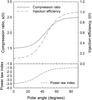 |
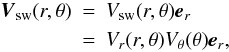
Fig. 1 The top panel shows both the latitude compression ratio s(θ) (solid line) and normalized ACR injection efficiency (I(θ), dashed line) as a function of polar angle. Both of these quantities have a maximum in the equatorial regions and decrease towards the polar regions. The bottom panel shows the 1D Fermi I acceleration power law spectral index, as calculated using Eq. (8), for the values of s(θ) shown in the top panel. |
Adopting a latitude dependent s(θ) has further consequences for ACR acceleration, as the well known Fermi I acceleration power law is highly dependent on s(θ). For a 1D planar shock, the accelerated Fermi I power law has the form

with
Using the values of s(θ) as calculated via Eq. (6), this leads to a hard accelerated spectrum in the equatorial regions (γ(90°) = − 1.5) but softening towards the polar regions (γ(0°) = − 3.5). The bottom panel of Fig. 1 shows γ(θ) as a function of polar angle, with the values of s(θ) given by Eq. (6).
Similar transitions for s(θ) and I(θ) were also introduced in previous modulation studies by Ngobeni & Potgieter (2008) and Langner & Potgieter (2006). Together, this choice of parameters form a region of preferred acceleration at the TS near the equatorial regions, the effect of which will be investigated later in this paper. Voyager 1 and 2 observations during the last A > 0 period show some evidence for higher ACR intensities at low latitudes (Hill & Hamilton 2003; Hill 2004).
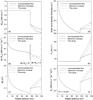 |
Fig. 2 The heliosheath plasma profiles assumed in this study, under the assumption of a radial solar wind speed given by Eq. (9). Panel a) shows the assumed Vsw profile, with panel b) showing the resulting ∇·Vsw. Panels c) − e) show the magnetic field magnitude, solar wind density and Alfvén speed profiles, respectively. Panel f) shows the calculated momentum diffusion coefficient from Eq. (3) at a rigidity of P = 1 GV. For all cases, results are shown in the equatorial plane, and for three different assumptions of Vsw namely, the profile according to Eq. (10), incompressible flow with Vsw ∝ r-2 and an assumed maximal decrease of Vsw ∝ r-6. The TS is located at rTS = 94 AU. |
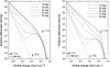 |
Fig. 3 To emphasize the effect of choosing a latitude dependent s(θ) and I(θ), the figure shows the resulting Fermi I accelerated TS spectra at different polar angles. The left panel shows results for the qA > 0 magnetic polarity cycle, while the right is for the qA < 0 cycle. Also shown are the expected Fermi I power law decreases in intensity (dotted lines) from Eqs. (7) and (8) for a planar shock, at the poles and in the equatorial plane. |
3. Heliosheath plasma profiles
In this study, the solar wind velocity is assumed to have the form
which is directed radially outwards. Although recent observations from Richardson et al. (2009) show that Vsw is already developing a latitudinal component at the V2 position, we argue that Eq. (9) is still a good approximation in the inner heliosheath, and specifically in the nose direction of the heliosphere. Results from Pogorelov et al. (2009) suggest that non-radial solar wind flow may become dominant beyond ~120 AU along the Voyager spacecraft trajectories. In Eq. (9), Vθ(θ) represents the latitudinal variation of Vsw. As solar minimum conditions are assumed throughout, Vθ(θ) changes the solar wind speed from 400 km s-1 in the equatorial regions to 800 km s-1 in the polar regions, in accordance with the Ulysses observations of Phillips et al. (1994).
Inside the TS a constant solar wind speed of Vr(r,θ) = 400 km s-1 is assumed in the equatorial plane, dropping by a factor of s(θ) across the TS. A shock precursor, also observed by V1 (Decker et al. 2005) and V2 (Richardson et al. 2008), with a scale length of 1.2 AU forms a semi-discontinuous TS structure (le Roux et al. 1996).
In the heliosheath, the form of Vr(r,θ) is still unclear, and the following profile is assumed
![\begin{equation} % V_r(r,\theta) = \frac{V_{\rm sw,0}}{s(\theta)} \left[ \frac{r}{r_{\rm TS}} \right]^{a(r)}, \label{Eq:solarwind_heliosheath} \end{equation}](/articles/aa/full_html/2010/14/aa14528-10/aa14528-10-eq74.png)
where a(r) is a linear function resulting in a(rTS) = −2 and a(rHP) = −6 and Vsw,0 the upstream value of the solar wind speed. This form of Vr(r,θ) is based on the HD results of Ferreira et al. (2007), where the steeper than r-2 decrease in the solar wind speed in this region (as is expected for a purely radial incompressible solar wind flow) is due to change exchange (Fahr et al. 2000). Similar solar wind profiles were also observed in other HD models, e.g. Fahr et al. (2000), Florinski et al. (2004) and Ferreira et al. (2008). The radial dependence of Vsw, as calculated with Eq. (10), is shown in panel (a) of Fig. 2, in the equatorial plane. Two other heliosheath profiles are shown for comparison, namely the incompressible case Vsw ∝ r-2 and an assumed maximal decrease of Vsw ∝ r-6. All plasma profiles in this section are shown for these three cases. The importance of a realistic Vsw profile in the heliosheath lies in the fact that the solar wind divergence ∇·Vsw governs the adiabatic term in Eq. (1). Inside the TS, ∇·Vsw > 0 leads to adiabatic cooling occurring in this region. For ∇·Vsw < 0, as implied by Eq. (10), this leads to adiabatic heating occurring in the heliosheath (see e.g. Langner et al. 2006; Zhang 2006). The resulting ∇·Vsw for the three different cases of Vsw is shown in panel (b) of Fig. 2. Note that the incompressible case in the heliosheath, ∇·Vsw = 0, leads to no energy losses/gains in this region. For Vsw given by Eq. (10), ∇·Vsw ~ 0 directly beyond the TS, and no heating is expected there. Near the HP however, ∇·Vsw < 0 is large and significant energy gains are expected.
The HMF is assumed Parkerian (Parker 1958), but modified in the polar regions according to the work of Jokipii & Kóta (1989). Furthermore, it is assumed that the HMF spiral and the HCS structure extend into the heliosheath, with the frozen in HMF conditions assumed to be satisfied. The HMF magnitude thus scales as B ~ 1/ (rVsw) in this region. Using Vsw from Eq. (10), this translates to a B ~ r increase near the TS, but steepening to B ~ r5 near the HP. This is in accordance with the B ~ r increase observed in the inner heliosheath (Burlaga et al. 2008). The radial dependence of B, for the different scenarios of Vsw discussed previously, are shown in panel (c) of Fig. 2, in the equatorial plane.
The solar wind mass density ρ is approximated by assuming conservation of the solar wind mass flux, i.e. ρ(r,θ)Vsw(r,θ)r2 = const., from which the Alfvén speed is calculated as
with μ0 the permittivity of free space. Panels (d) and (e) of Fig. 2 show the radial dependence of both ρ and VA, in the equatorial plane of the heliosphere. The Alfvén speed is characterized by the rather flat profile inside the TS with VA ~ 35 km s-1. This is because B ~ r-1 (if r ≫ 1 AU) and ρ ~ r-2. Inside the heliosheath however,  , being highly dependent on the assumed Vsw profile. For the incompressible case, VA ~ r in the heliosheath and VA stays relatively low throughout the heliosheath. For this case Fermi II acceleration is thought not to be very effective, due to the dependence on VA (Eq. (3)), as also concluded by Moraal et al. (2006). For the profile according to Eq. (10) however, VA shows a very large increase in the heliosheath and especially near the HP. This large increase makes Fermi II acceleration a viable re-acceleration process in this region (Ferriera et al. 2007). This can also be seen from the radial profile of κP, shown in panel (f) of Fig. 2, at a rigidity of P = 1 GV.
4. Modelling results
4.1. Latitude dependent s(θ) and I(θ)
To emphasize the effect of choosing both a latitude dependent s(θ) and I(θ), Fig. 3 shows the resulting Fermi I accelerated TS spectra at different co-latitudes (polar angles) along the TS. The left panel is for the qA > 0 magnetic polarity cycle, while the right is for the qA < 0. Note that the results described in this paragraph do not include Fermi II acceleration, which is discussed in the following section, together with adiabatic heating. The effect of I(θ) is clearly visible at the low energy regime (~10-6 GeV nuc-1), where the O* intensities are generally a factor I(θ) lower than those at the equatorial plane. At higher energies however, the effect of s(θ) is dominant. For low energies, E < 0.1 MeV nuc-1, the well known Fermi I accelerated power law is obtained when compared to the 1D planar shock case at θ = 0°, 90°, with the spectral index being dependent on the polar angle as expected through Eqs. (7) and (8). Near the equatorial plane, θ > 60°, this power law persists up to ~10 MeV nuc-1 in the equatorial plane, where the ACR roll-over is observed. This almost exponential decay in intensity is believed to occur predominantly due to the curvature of the TS (Steenberg & Moraal 1999) leading to ineffective Fermi I acceleration above these energies. Near the polar regions however, the spectra exhibit a highly modulated form for E > 0.1 MeV nuc-1. This is due to high energy particles, accelerated at the equatorial regions, diffusing and/or drifting towards the polar regions, leading to an excess of high energy particles at the polar regions not accelerated there locally. The dominant process responsible for this poleward migration of particles is poleward diffusion. Drifts however facilitate this movement of particles during the qA > 0 magnetic polarity cycle, but hinder it during the qA < 0. This leads to HMF polarity dependent TS spectra. A curious feature is the modelled HMF polarity dependent spectra at the equatorial plane, with a clear intensity enhancement forming at E ~ 10 MeV nuc-1, in the qA < 0 cycle. This too is believed to be due to drift effects (Florinski & Jokipii 2003) and warrants further investigation, but falls beyond the scope of this work.
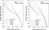 |
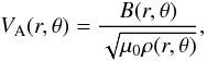
Fig. 4 Modelled O* energy spectra in the heliosheath for the qA > 0 (left panel) and qA < 0 (right panel) magnetic polarity cycles. The results are shown at the TS and in 10 AU intervals up to the HP at a polar angle of 55°. The results include ACR re-acceleration in the heliosheath via adiabatic heating and momentum diffusion. |
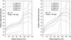 |
Fig. 5 Modelled O* intensities as a function of radial distance at various energies for both polarity cycles at a polar angle of 55°. The position of the TS is indicated by the vertical line. The grey lines correspond to only adiabatic heating occurring in the heliosheath (i.e. κP,0 = 0.0), while the black lines include Fermi II acceleration (i.e. κP,0 = 0.5). The vertical dashed line shows the approximate position (at r = 120 AU) where non-radial solar wind flow may begin to dominate. |
4.2. Momentum diffusion and adiabatic heating
Figure 4 shows the modelled O* energy spectra, with the inclusion of both a latitude dependent s(θ) and I(θ), as well as adiabatic heating and Fermi II acceleration included in the modulation model for both the qA > 0 (left panel) and qA < 0 (right panel) HMF polarity cycles. The spectra are shown at a polar angle of 55°, the approximate position of the V1 spacecraft, at the TS and in 10 AU intervals up to the HP. The results for both polarity cycles are qualitatively similar, being more pronounced in the qA < 0 cycle. The resulting energy spectra are also comparable to those of previous studies (Zhang et al. 2006; Ferreira et al. 2007) which included Fermi II acceleration for other ACR species. The modulated form of the high energy TS spectra was discussed previously, although the inclusion of Fermi II acceleration further enhances this form. It is well known that adiabatic heating occurring in the heliosheath generally leads to increasing ACR intensities away from the TS and peaking well inside the heliosheath (Langner et al. 2006). The inclusion of Fermi II acceleration into the modulation model generally leads to a further increase in intensity. Unlike adiabatic heating, momentum diffusion also affects the spectral shape of the heliosheath spectra significantly. The modulated TS spectra seem to unfold towards the HP, exhibiting an almost power law form near the HP, with a spectral index much harder than at the TS. Also notable is that the intensity enhancement (or “bump”) in the TS spectra at ~1 MeV nuc-1, moves towards lower energies nearer to the HP, characteristic of momentum diffusion. At 134 AU this enhancement is replaced by a very sharp decrease in intensity at low energies. This cut-off was also observed in previous modulation studies, which included Fermi II acceleration (e.g. Ferreira et al. 2007). Not shown in this figure, the O* energy spectra in the inner heliosphere remain relatively unchanged by the inclusion of momentum diffusion into the modulation model. This is because these spectra are dominated by the adiabatic regime at low energies, leading to the j ∝ E adiabatic spectral form observed at 1 AU.
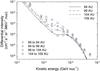 |
Fig. 6 A comparison between modelled energy spectra and V1 O* observations in the heliosheath. The modelling results are for the qA < 0 magnetic polarity cycle and shown at a polar angle of 55°. The data symbols are long term averaged O energy spectra for four 5-AU-wide radial ranges (as shown) and reveal the energetic particle behaviour at V1, immediately upstream of the TS and in the heliosheath. From smallest to largest distances the four periods are 2003/220-2004/346, 2004/353-2006/124, 2006/125-2007/259, and 2007/260-2009/028 (where the year and day of year are indicated). Note that the statistical uncertainties are smaller than the symbol sizes. The modelled spectra are plotted at positions near the centre of each radial bin, as given. |
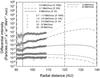 |
Fig. 7 A comparison between modelled O* intensities and V1 observations, shown as a function of radial distance. The V1 energetic O intensities are averaged over 0.10-AU-wide intervals and plotted against radial distance for five energy ranges (as shown). Statistical uncertainties are not shown, but are below approximately 10% (smaller than the symbol size) after the TS crossing and 50% (comparable to the symbol size) immediately upstream. For some energies both the modelled and observed intensities are multipled by scaling factors for clarity, as indicated in the legend. The position of the TS is indictated by the vertical line. The model results are shown at a polar angle of 55° for the qA < 0 magnetic polarity cycle, as is appropriate for the corresponding observations. The vertical dashed line shows the approximate position (at r = 120 AU) where non-radial solar wind flow may begin to dominate. |
Figure 5 shows modelled O* intensities as a function of radial distance for both polarity cycles at various energies, at a polar angle of 55°. Again the results for both polarity cycles are qualitative similar and comparable to those of previous studies. At E < 6 MeV nuc-1, both adiabatic heating and Fermi II acceleration causes O* intensities to increase into the heliosheath. For E > 6 MeV nuc-1, both of these processes are however ineffective and the O* heliosheath intensities are characterized by flat (qA > 0 cycle) or decreasing (qA < 0 cycle) intensities. From Fig. 2 is is expected that both of these processes are most effective in the outer heliosheath, i.e. close to the HP. This can be seen most clearly in the very low, 0.1 MeV nuc-1, intensities, being relatively flat directly beyond the TS but increasing drastically (by a factor of ~100) towards the HP. Due to the outward convection of Vsw, being dominant at these low energies, the low energy particles, re-accelerated near the HP, are unable to diffuse back towards the TS. At E > 0.1 MeV nuc-1, these re-accelerated particles are able to diffuse back towards the TS, leading to higher O* intensities throughout the heliosheath.
The increase in O* intensities towards the HP is dependent, amongst others, on the position of the HP (Webber et al. 2009; Swisdak et al. 2010), i.e. the thickness of the heliosheath, as well as the boundary conditions assumed at the HP. The results of Fig. 5 show a steep decrease in O* intensities near the HP. This is due to the absorbing boundary condition assumed there in the modulation model. A more accurate description however seems to be a free-escape boundary (Scherer et al. 2008), where ACRs are allowed to propagate into the interstellar medium. The effect of this still needs to be examined in more detail.
4.3. Comparison with observations
In Figs. 6 and 7 we show comparisons between modelled (including adiabatic heating and cooling, Fermi II acceleration, and the latitudinally varying injection efficiency and shock strength given by Eqs. (5) and (6)) O* intensities and V1 observations immediately upstream of the TS and in the heliosheath.
The measurements were made with the Low Energy Charged Particle Instrument (LECP; Krimigis et al. 1977) on board the V1 spacecraft. The LECP instruments are solid-state detector (SSD) telescopes that measure the composition and intensities of ions at V1 and V2. Clean elemental separation is obtained by measuring the kinetic energy deposited in adjacent SSDs by an ion as it passes into the instrument. In Figs. 6 and 7 we show 26-day averaged V1 oxygen intensities observed over the 315° × 60° LECP field of view.
Figure 6 compares O* energy spectra, with very good agreement between modelling and experimental results. The modulation model discussed in this paper not only reproduces the observed modulated form of the TS spectrum, but also the unfolding of this spectrum as V1 moves into the heliosheath. A slight discrepancy exists between the modelled results and the observations above ~30 MeV nuc-1. This can be explained by incorporating the effects of multiple charged O* into the modulation model (Strauss et al. 2010).
A good agreement also exists when O* intensities are compared to V1 observations as a function of radial distance (Fig. 7). For all energies the modelling results and observations show the same trends, with increasing O* intensities below ~10 MeV nuc-1 and rather flat profiles for higher energies. It must also be noted that temporal effects are not presently included in the modulation model, but are probably not insignificant in the observations.
5. Summary and conclusions
In this paper, a comprehensive ACR acceleration and transport model was discussed and applied to the study of O*.
It was shown that a combination of s(θ) and I(θ) leads to a modulated form of the accelerated Fermi I TS spectra. The form of s(θ) and I(θ), as used in this study, leads to a region of preferred acceleration at the TS near the equatorial plane of the heliosphere. High energy particles are then able to diffuse/drift along the TS to higher latitudes, reproducing the observed modulated form of this spectrum at intermediate latitudes. This is in contrast to the model of McComas & Schwadron (2006) where ACRs are accelerated primarily at the flanks of the heliosphere, although the resulting spectra from both of these models are fairly similar. This is also in contrast to an earlier model of Jokipii (1986) where ACRs were accelerated primarily in the polar regions of the heliosphere.
This modulated TS spectra then unfolds further into the heliosheath due to a combination of Fermi II acceleration and adiabatic heating. Both of these processes are most effective in the outer heliosheath, i.e. close to the HP. O* accelerated at the TS (through diffusive shock acceleration), diffuse outwards towards the HP where they are re-accelerated by means of these processes, and then diffuse back towards the TS, modulating the energy spectra throughout the heliosheath. It was also shown that low energy re-accelerated ACRs are unable to diffuse back towards the TS due to outwards convection by the solar wind.
Diffusive shock acceleration at the TS is needed to set up a “source” spectrum at the TS, which is further modulated in the heliosheath. In contrast to Kallenbach et al. (2009), it is thus believed that Fermi I acceleration at the TS is needed for re-acceleration to occur near the HP. The viability of momentum diffusion is however dependent on e.g. the Alfvén speed in the heliosheath, which in turn is dependent on the solar wind profile. The exact form of this profile is still uncertain, with the assumed profile used in this paper leading to a large increase of VA into the heliosheath, resulting in more efficient Fermi II acceleration in this region. A similar conclusion was made by Chalov et al. (2007), albeit using a different approach.
Comparison between modelling results and observations were shown in Figs. 6 and 7. A very good agreement with the V1 heliosheath observations is achieved, with the modulation model accurately reproducing both the observed spectral form and increase in O* intensities into the heliosheath.
It is concluded that Fermi II acceleration, occurring predominantly in the outer regions of the inner heliosheath, is a viable ACR re-acceleration mechanism under certain realistic assumptions for heliosheath plasma profiles, and by incorporating this process into a modulation model we are successful in reproducing O* observations in the heliosheath.
Acknowledgments
The authors wish to thank K. Scherer and W. R. Webber for helpful and informative research discussions.
References
- Burger, R. A., Potgieter, M. S., & Heber, B. 2000, J. Geophys. Res., 105, 27447 [Google Scholar]
- Burger, R. A., Krüger, T. P. J., Hitge, M., & Engelbrecht, N. E. 2008, ApJ, 674, 511 [NASA ADS] [CrossRef] [Google Scholar]
- Burlaga, L. F., Ness, N. F., Acuña, M. H., et al. 2005, Science, 309, 2027 [NASA ADS] [CrossRef] [PubMed] [Google Scholar]
- Burlaga, L. F., Ness, N. F., & Acuña, M. H. 2008, AIP Conf. Ser., 1039, 329 [NASA ADS] [CrossRef] [Google Scholar]
- Chalov, S. V., Fahr, H. J., & Malama, Y. G. 2007, Ann. Geophys., 25, 575 [Google Scholar]
- Drake, J. F., Opher, M., Swisdak, M., & Chamoun, J. N. 2010, ApJ, 709, 963 [NASA ADS] [CrossRef] [Google Scholar]
- Fahr, H. J., Kausch, T., & Scherer, H. 2000, A&A, 357, 268 [NASA ADS] [Google Scholar]
- Decker, R. B., Krimigis, S. M., Roelof, E. C., et al. 2005, Science, 309, 2020 [NASA ADS] [CrossRef] [PubMed] [Google Scholar]
- Decker, R. B., Krimigis, S. M., Roelof, E. C., et al. 2008, Nature, 454, 67 [NASA ADS] [CrossRef] [PubMed] [Google Scholar]
- Ferreira, S. E. S., Potgieter, M. S., & Scherer, K. 2007, J. Geophys. Res., 112, 11101 [Google Scholar]
- Ferreira, S. E. S., Scherer, K., & Potgieter, M. S. 2008, Adv. Space Res., 41, 351 [NASA ADS] [CrossRef] [Google Scholar]
- Fisk, L. A., & Gloeckler, G. 2009, Adv. Space Res., 43, 1471 [NASA ADS] [CrossRef] [Google Scholar]
- Fisk, L. A., Kozlovsky, B., & Ramaty, R. 1974, ApJ, 190, L35 [NASA ADS] [CrossRef] [Google Scholar]
- Florinski, V., & Jokipii, J. R. 2003, ApJ, 591, 454 [NASA ADS] [CrossRef] [Google Scholar]
- Florinski, V., & Pogorelov, N. V. 2009, ApJ, 701, 642 [NASA ADS] [CrossRef] [Google Scholar]
- Florinski, V., & Zank, G. P. 2006, Geophys. Res. Lett., 33, 15110 [NASA ADS] [CrossRef] [Google Scholar]
- Florinski, V., Zank, G. P., Jokipii, J. R., Stone, E. C., & Cummings, A. C. 2004, ApJ, 610, 1169 [NASA ADS] [CrossRef] [Google Scholar]
- Florinski, V., Balogh, A., Jokipii, J. R., et al. 2009, Space Sci. Rev., 143, 57 [NASA ADS] [CrossRef] [Google Scholar]
- Hill, M. E. 2004, in Physics of the Outer Heliosphere, ed. V. Florinski, N. V. Pogorelov, & G. P. Zank, 719, 156 [Google Scholar]
- Hill, M. E., & Hamilton, D. C. 2003, Proc. 28th ICRC, 7, 3969 [Google Scholar]
- Jokipii, J. R. 1986, J. Geophys. Res., 91, 2929 [NASA ADS] [CrossRef] [Google Scholar]
- Jokipii, J. R. 1996, ApJ, 466, L47 [NASA ADS] [CrossRef] [Google Scholar]
- Jokipii, J. R., & Kóta, J. 1989, J. Geophys. Res., 16, 1 [Google Scholar]
- Kallenbach, R., Hilchenbach, M., Chalov, S. V., le Roux, J. A., & Bamert, K. 2005, A&A, 439, 1 [NASA ADS] [CrossRef] [EDP Sciences] [Google Scholar]
- Kallenbach, R., Bamert, K., & Hilchenbach, M. 2009, ASTRA, 5, 49 [Google Scholar]
- Krimigis, S. M., Bostrom, C. O., Armstrong, T. P., et al. 1977, Space Sci. Rev., 21, 329 [NASA ADS] [CrossRef] [Google Scholar]
- Langner, U. W., & Potgieter, M. S. 2006, in Acceleration of galactic and anomalous cosmic rays in the heliosheath, ed. J. Heerikhuisen, V. Florinski, G. P. Zank, et al. (New York: AIP), 858, 233 [Google Scholar]
- Langner, U. W., Potgieter, M. S., & Webber, W. R. 2003, J. Geophys. Res., 108, 8039 [CrossRef] [Google Scholar]
- Langner, U. W., Potgieter, M. S., & Webber, W. R. 2004, Adv. Space Res., 34, 138 [NASA ADS] [CrossRef] [Google Scholar]
- Langner, U. W., Potgieter, M. S., Fichtner, H., & Borrmann, T. 2006, J. Geophys. Res., 111, A101106 [Google Scholar]
- Lazarian, A., & Opher, M. 2009, ApJ, 703, 8 [NASA ADS] [CrossRef] [Google Scholar]
- Lee, M. A., Fahr, H. J., & Kucharek, H. 2009, Space Sci. Rev., 146, 275 [NASA ADS] [CrossRef] [Google Scholar]
- le Roux, J. A., Potgieter, M. S., & Ptuskin, V. S. 1996, J. Geophys. Res., 101, 4791 [NASA ADS] [CrossRef] [Google Scholar]
- le Roux, J. A., Zank, G. P., & Ptuskin, V. S. 1999, J. Geophys. Res., 104, 24845 [Google Scholar]
- McComas, D. J., & Schwadron, N. A. 2006, Geophys. Res. Lett., 33, 4102 [NASA ADS] [CrossRef] [Google Scholar]
- Moraal, H., Caballero-Lopez, R. A., McCracken, K. G., et al. 2006, in Physics of the Inner Heliosheath, ed. J. Heerikhuisen, V. Florinski, G. P. Zank, et al., 858, 219 [Google Scholar]
- Minnie, J., Bieber, J. W., Matthaeus, W. H., et al. 2007, ApJ, 670, 1149 [NASA ADS] [CrossRef] [Google Scholar]
- Ngobeni, M. D., & Potgieter, M. S. 2008, Adv. Space Res., 41, 373 [Google Scholar]
- Parker, E. N. 1958, ApJ, 128, 664 [Google Scholar]
- Parker, E. N. 1965, Planet. Space. Sci., 13, 9 [NASA ADS] [CrossRef] [Google Scholar]
- Pesses, M. E., Eichler, D., & Jokipii, J. R. 1981, ApJ, 246, L85 [NASA ADS] [CrossRef] [Google Scholar]
- Phillips, J. L., Bame, S. J., Barnes, A., et al. 1994, Geophys. Res. Lett., 22, 3301 [Google Scholar]
- Pogorelov, N. V., Heerikhuisen, J., Zank, G. P., Mitchell, J. J., & Cairns, I. H. 2009, Adv. Space. Res., 44, 1337 [NASA ADS] [CrossRef] [Google Scholar]
- Potgieter, M. S. 1989, Adv. Space. Res., 9, 1989 [Google Scholar]
- Potgieter, M. S. 2008, Adv. Space. Res., 41, 245 [Google Scholar]
- Richardson, J. D., Kasper, J. C., Wang, C., Belcher, J. W., & Lazarus, A. J. 2008, Nature, 454, 63 [NASA ADS] [CrossRef] [PubMed] [Google Scholar]
- Richardson, J. D., Stone, E. C., Kasper, J. C., Belcher, J. W., & Decker, R. B. 2009, J. Geophys. Res., 36, L10102 [Google Scholar]
- Ruciński, D., Cummings, A. C., Gloeckler, G., et al. 1996, Space. Sci. Rev., 78, 73 [Google Scholar]
- Scherer, K., & Fahr, H.-J. 2009, A&A, 495, 631 [NASA ADS] [CrossRef] [EDP Sciences] [Google Scholar]
- Scherer, K., Ferreira, S. E. S., Potgieter, M. S., & Fichtner, H. 2006, in Physics of the Inner Heliosheath, ed. J. Heerikhuisen, V. Florinski, G. P. Zank, et al., 858, 20 [Google Scholar]
- Scherer, K., Fichtner, H., Ferreira, S. E. S., Büsching, I., & Potgieter, M. S. 2008, ApJ, 680, L105 [NASA ADS] [CrossRef] [Google Scholar]
- Steenberg, C. D., & Moraal, H. 1999, J. Geophys. Res., 104, 24879 [Google Scholar]
- Stone, E. C., Cummings, A. C., McDonald, F. B., et al. 2005, Science, 309, 2017 [NASA ADS] [CrossRef] [PubMed] [Google Scholar]
- Strauss, R. D., Potgieter, M. S., & Ferrreira, S. E. S. 2010, A&A, 513, A24 [NASA ADS] [CrossRef] [EDP Sciences] [Google Scholar]
- Swisdak, M., Opher, M., Drake, J. F., & Alouani Bibi, F. 2010, ApJ, 710, 1769 [NASA ADS] [CrossRef] [Google Scholar]
- Webber, W. R., Cummings, A. C., McDonald, F. B., et al. 2007 J. Geophys. Res., 112, A06105 [CrossRef] [Google Scholar]
- Webber, W. R., Cummings, A. C., McDonald, F. B., et al. 2009, J. Geophys. Res., 114, A13 [Google Scholar]
- Zhang, M. 2006, in Physics of the Inner Heliosheath, ed. J. Heerikhuisen, V. Florinski, G. P. Zank, et al., 858, 226 [Google Scholar]
All Figures
|
Fig. 1 The top panel shows both the latitude compression ratio s(θ) (solid line) and normalized ACR injection efficiency (I(θ), dashed line) as a function of polar angle. Both of these quantities have a maximum in the equatorial regions and decrease towards the polar regions. The bottom panel shows the 1D Fermi I acceleration power law spectral index, as calculated using Eq. (8), for the values of s(θ) shown in the top panel. |
| In the text | |
|
Fig. 2 The heliosheath plasma profiles assumed in this study, under the assumption of a radial solar wind speed given by Eq. (9). Panel a) shows the assumed Vsw profile, with panel b) showing the resulting ∇·Vsw. Panels c) − e) show the magnetic field magnitude, solar wind density and Alfvén speed profiles, respectively. Panel f) shows the calculated momentum diffusion coefficient from Eq. (3) at a rigidity of P = 1 GV. For all cases, results are shown in the equatorial plane, and for three different assumptions of Vsw namely, the profile according to Eq. (10), incompressible flow with Vsw ∝ r-2 and an assumed maximal decrease of Vsw ∝ r-6. The TS is located at rTS = 94 AU. |
| In the text | |
|
Fig. 3 To emphasize the effect of choosing a latitude dependent s(θ) and I(θ), the figure shows the resulting Fermi I accelerated TS spectra at different polar angles. The left panel shows results for the qA > 0 magnetic polarity cycle, while the right is for the qA < 0 cycle. Also shown are the expected Fermi I power law decreases in intensity (dotted lines) from Eqs. (7) and (8) for a planar shock, at the poles and in the equatorial plane. |
| In the text | |
|
Fig. 4 Modelled O* energy spectra in the heliosheath for the qA > 0 (left panel) and qA < 0 (right panel) magnetic polarity cycles. The results are shown at the TS and in 10 AU intervals up to the HP at a polar angle of 55°. The results include ACR re-acceleration in the heliosheath via adiabatic heating and momentum diffusion. |
| In the text | |
|
Fig. 5 Modelled O* intensities as a function of radial distance at various energies for both polarity cycles at a polar angle of 55°. The position of the TS is indicated by the vertical line. The grey lines correspond to only adiabatic heating occurring in the heliosheath (i.e. κP,0 = 0.0), while the black lines include Fermi II acceleration (i.e. κP,0 = 0.5). The vertical dashed line shows the approximate position (at r = 120 AU) where non-radial solar wind flow may begin to dominate. |
| In the text | |
|
Fig. 6 A comparison between modelled energy spectra and V1 O* observations in the heliosheath. The modelling results are for the qA < 0 magnetic polarity cycle and shown at a polar angle of 55°. The data symbols are long term averaged O energy spectra for four 5-AU-wide radial ranges (as shown) and reveal the energetic particle behaviour at V1, immediately upstream of the TS and in the heliosheath. From smallest to largest distances the four periods are 2003/220-2004/346, 2004/353-2006/124, 2006/125-2007/259, and 2007/260-2009/028 (where the year and day of year are indicated). Note that the statistical uncertainties are smaller than the symbol sizes. The modelled spectra are plotted at positions near the centre of each radial bin, as given. |
| In the text | |
|
Fig. 7 A comparison between modelled O* intensities and V1 observations, shown as a function of radial distance. The V1 energetic O intensities are averaged over 0.10-AU-wide intervals and plotted against radial distance for five energy ranges (as shown). Statistical uncertainties are not shown, but are below approximately 10% (smaller than the symbol size) after the TS crossing and 50% (comparable to the symbol size) immediately upstream. For some energies both the modelled and observed intensities are multipled by scaling factors for clarity, as indicated in the legend. The position of the TS is indictated by the vertical line. The model results are shown at a polar angle of 55° for the qA < 0 magnetic polarity cycle, as is appropriate for the corresponding observations. The vertical dashed line shows the approximate position (at r = 120 AU) where non-radial solar wind flow may begin to dominate. |
| In the text | |
Current usage metrics show cumulative count of Article Views (full-text article views including HTML views, PDF and ePub downloads, according to the available data) and Abstracts Views on Vision4Press platform.
Data correspond to usage on the plateform after 2015. The current usage metrics is available 48-96 hours after online publication and is updated daily on week days.
Initial download of the metrics may take a while.