© ESO, 2010

1. Introduction

Classical T Tauri stars (CTTS) are young low-mass stars ( ≤ 2   M_⊙), with typical spectral types between F and M, which are still accreting material from a circumstellar disk. These stars show emission lines ranging from the X-ray to the IR part of the spectrum, and the most commonly observed one is the Hα line. Today, the most accepted scenario used to explain the accretion phenomenon in these young stellar objects is the magnetospheric accretion (MA) mechanism. In this scenario, a strong stellar magnetic field truncates the circumstellar disk near the co-rotation radius, and the matter in the disk inside this region free-falls onto the stellar photosphere following magnetic field lines. When the plasma reaches the end of the accretion column, the impact with the stellar surface creates a hot spot, where its kinetic energy is thermalized (e.g., Camenzind 1990; Koenigl 1991). The gas is heated to temperatures of  ≃ 10⁶K in the shock, which then emits strongly in the X-rays. Most of the X-rays are then reabsorbed by the accretion column, and re-emitted as the blue and ultraviolet continuum excess (e.g., Calvet & Gullbring 1998), which can be observed in CTTS.

The magnetospheric accretion paradigm is currently strongly supported by observations. Magnetic field measurements in CTTS yielded strengths on their surfaces on the order of 10³   G persistently over time scales of years (Johns-Krull et al. 1999; Symington et al. 2005; Johns-Krull 2007). These fields are strong enough to disrupt the circumstellar disk at some stellar radii outside the stellar surface. Classical T Tauri stars also exhibit inverse P Cygni (IPC) profiles, mostly in the Balmer lines that arise from the higher excitation levels, and some metal lines which are directly linked to the MA phenomenon (Edwards et al. 1994). These lines are broadened to velocities on the order of hundreds of kms^-1, which is evidence of free-falling gas from a distance of some stellar radii above the star. There is also an indication of line profile modulation by the stellar rotation period (e.g., Bouvier et al. 2007).

However, the MA scenario is only partially successful in explaining the features observed in line profiles of CTTS. Observational studies show evidence of outflows in these objects, which are inferred by the blue-shifted absorption features that can be seen in some of the Balmer and Na D lines (e.g., Alencar & Basri 2000). Bipolar outflows leaving these objects have been observed down to scales of  ≃ 1AU (e.g., Takami et al. 2003; Appenzeller et al. 2005). On larger scales, HST observations of HH30 (e.g., Burrows et al. 1996) could trace a bipolar jet to within  ≲ 30AU of the star. This suggests a greater complexity of the circumstellar environment, in which the MA model is only a piece of the puzzle.

The observed jets are believed to be highly collimated magneto-hydrodynamic disk winds which efficiently extract angular momentum and gravitational energy from the accretion disk. Blandford & Payne (1982, hereafter BP) were the first to propose the use of a disk wind to explain the origin of jets from accreting disks around a black hole, and soon after Pudritz & Norman (1983, 1986) proposed a similar mechanism for the origin of the protostellar jets. Bacciotti et al. (2003), using high resolution spectro-imaging and adaptative optics methods on protostellar jets, observed what seems to be rotational motion inside these jets, and also an onion-like velocity structure where the highest speeds are closer to the outflow axis. Their work strongly corroborates the idea of the origin of jets as centrifugally driven MHD winds from extended regions of their accretion disks. A correlation between jets, infrared excess, and the accretion process has been observed (Cabrit et al. 1990; Hartigan et al. 1995), which indicates a dependence between the outflow and inflow of matter in CTTS. Disk wind theories show the existence of a scale relation between the disk accretion (Ṁ_acc) and the mass loss rates (Ṁ_loss) (Pelletier & Pudritz 1992). Observations have confirmed this relation (Hartmann 1998), and both have agreed that in CTTS the typical value for this relation is Ṁ_loss / Ṁ_acc ≃ 0.1. Another model widely used to explain the outflows and the protostellar jets is called the X-wind model (Shu et al. 1994; Cai et al. 2008), which states that instead of originating in a wider region of the accretion disk, the outflow originates in a very constrained region around the so called “X-point”, which is at the Keplerian co-rotation radius of the stellar magnetosphere.

Many developments in MHD time-dependent numerical models have been made in the last years. Zanni et al. (2007) were able to reproduce the disk-wind lauching mechanism and jet formation from a magnetized accretion disk with a resistive MHD axisymmetric model showing the system evolution over tens of rotation periods. They were able to find a configuration in which a slowly evolving outflow leaving the inner part of the accretion ring (from  ~ 0.1 to  ~ 1 AU) was formed, when using a high disk magnetic resistivity. Murphy et al. (2010) showed that it was possible to form a steady disk wind followed by a self-contained super-fast-magnetosonic jet using a weakly magnetized accretion disk. Their numerical solution remained steady for almost a thousand Keplerian orbits. Both models help to strengthen the disk wind scenario. Romanova et al. (2009), however, showed that it is also possible to numerically simulate the launching of a thin conical wind, which is similar in some respects to an X-wind, considering only an axisymmetric stellar dipolar magnetic field around a slowly rotating star. A fast axial jet component also appears in the case of a fast rotating star. Their conical wind also shows some degree of collimation, but, as stated by Romanova et al. (2009), this collimation may not be enough to explain the observed well-collimated jets.

Radiative transfer models were used to calculate some of the line profiles that were observed in CTTS. The first of these models that used the MA paradigm, hereafter the HHC model, was proposed by Hartmann et al. (1994), and was based on a simple axisymmetric dipolar geometry for the accretion flow, using a two-level atom approximation under the Sobolev “resonant co-moving surfaces” approximation (SA). The model was later improved by the addition of the full statistical equilibrium equations in the code (Muzerolle et al. 1998), and finally including an exact integration of the line profile (Muzerolle et al. 2001). These models included only the magnetospheric and photospheric components of the radiation field and were partially successful in reproducing the observed line strengths and morphologies for some of the Balmer lines and Na D lines. In these models, the stellar photosphere and the inner part of the accretion disk partially occult the inflowing gas, and these occultations create an asymmetric blue-ward or red-ward emission peak, depending on the angle between the system symmetry axis, and the observer’s line of sight. The inflowing gas projected against hot spots on the stellar surface produces the IPC profiles that are sometimes observed.

Alencar et al. (2005) demonstrated that the observed Hα, Hβ, and Na D lines of RW Aur are better reproduced if a disk wind component arising from the inner rim of the accretion disk was added to these radiative transfer models, and it became clear that for more accurate predictions, these models should include that component. Kurosawa et al. (2006, henceforth KHS), were the first to use a self-consistent model where all these components were included, and could reproduce the wide variety of the observed Hα line profiles. Still, their cold MHD disk wind component used straight field lines, and some of which violate the launching conditions required by BP, which state that for an outflow to appear, its launching angle should be  > 30° away from the rotational axis of the system. Those infringing field lines in the KHS model were always the innermost ones, which, as we will show here, are responsible for the bulk of the Hα line profiles in the disk wind region.

The BP launching condition assumes a cold MHD flow, which is not always the case. In a more general situation, the thermal pressure term becomes important near the base of the outflow, and should not be neglected during the initial acceleration process, and thus it is possible to have a stable steady solution even if the launching angle exceeds 30°. The BP self-similar solution, although it is a very simple one, is able to describe mathematically and self-consistently the disk-wind launching mechanism and the further collimation of the disk wind to a jet by magnetic “hoop” stress. The self-similarity hypothesis becomes increasingly artificial farther away from the accretion disk, in the region where the jet is formed, but it remains valid near the accretion disk, where our calculations were performed.

In this work, we have included a disk wind component in the HHC model, using a modified version of the BP formulation. We then studied the parameter space of the improved model, while trying to identify how each parameter affected the calculated Hα profiles. In Sects. 2 and 3 we present the magnetospheric accretion, the disk wind and the radiative transfer models that were used as well as all the assumptions made to calculate our profiles. The model results are shown in Sect. 4, followed by a discussion in Sect. 5 and the conclusion in Sect. 6. A subsequent paper will focus on the modeling of the observed Hα lines for a set of classical T Tauri stars that exhibit different accretion and environmental characteristics.

2. Model structure

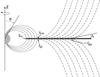Fig. 1 Not-to-scale sketch of the adopted axisymmetric geometry shown in the poloidal plane. The gray half-circle denotes the stellar photosphere, the dark rectangle represents the disk, which is assumed to be opaque and to extend to the innermost magnetic field line. The dotted lines represent the magnetosphere and its purely dipolar field lines, and the dash-dotted lines are parabolic trajectories that represent the disk wind streamlines. The inner and outer magnetospheric field lines intersect the disk at rmi and rmo, respectively, and the ring between rdi and rdo is the region where the disk wind is ejected. The inclination from the z-axis is given by θ, and ϑ0 is the disk-wind launching angle.

Our model structure comprises four components: the star, the magnetosphere, the accretion disk, and the disk wind. The center of the star is also the center of the model’s coordinate system, and the star rotates around the z-axis, which is the system’s axis of symmetry. We assume symmetry through the x-y plane. In our coordinate system, r is the radial distance from the center of the star, and θ is the angle between r and the z-axis. The modeled region is divided into a grid system, where 1 / 4 of the points are inside the magnetosphere, and the other 3 / 4 are part of the disk wind region. The star and accretion disk are assumed to be infinitely thick in the optical region of the spectrum, and as such can be said to emit as blackbodies, and act as boundaries in our model. Due to symmetry arguments, it is only necessary to calculate the velocity, density, and temperature fields in the first quadrant of the model. These values are rotated around the z-axis, and are then reflected through the x-y plane. The emission from the accretion disk in CTTS is neglected, because its temperature is usually much lower than the photospheric temperature of the star. A schematic diagram of the adopted geometry can be seen in Fig. 1.

The stellar surface is divided into two regions: the photosphere and the accretion shock (the region where the accruing gas hits the stellar photosphere). Unless otherwise stated, the stellar parameters used in the model are those of a typical CTTS, i.e. radius (R_∗), mass (M_∗) and effective temperature of the photosphere (T_ph) are 2.0   R_⊙, 0.5   M_⊙ and 4000K, respectively. When the gas hits the star, its kinetic energy is thermalized inside a radiating layer, and we consider that this layer emits as a single temperature blackbody. Because we assume axial symmetry, our accretion shock region can be regarded as two spherical rings near both stellar poles, and we assume their effective temperature (T_sh) to be 8000K, as used by Muzerolle et al. (2001). Although T_sh has been kept constant, it actually depends on the mass accretion rate. But it barely affects the Hα line profile and is only important when defining the continuum veiling levels.

2.1. Magnetospheric model

The basic assumption of this model is that accretion from the disk onto the CTTS is controlled by a dipole stellar magnetic field. This magnetic field is assumed to be strong enough to truncate the disk at some height above the stellar surface, and also to remain undisturbed by the ionized inflowing gas. The gas pressure inside the accretion funnel is assumed to be sufficiently low so that the infalling material free-falls onto the star.

For the considered axisymmetric flow, the streamlines can be described by $\mathit{r}\mathrm{=}{\mathit{r}}_{\mathrm{m}}{\sin }^{\mathrm{2}}\mathit{\theta ,}$(1)where r_m corresponds to the point where the stream starts at the disk surface, or, in other words, where θ = π / 2 (Ghosh et al. 1977). In this problem, we can use the ideal magneto-hydrodynamic (MHD) approximation, which assumes an infinite electrical conductivity inside the flow. According to this approximation, the flow is so strongly coupled to the magnetic field lines that the velocity of the inflowing gas is parallel to the magnetic field lines, and thus the poloidal component of the velocity is ${v}\mathrm{p}\mathrm{=}\mathrm{-}{3}_{\mathrm{p}}\left[\frac{\mathrm{3}{\mathit{y}}^{\mathrm{1}\mathit{/}\mathrm{2}}\mathrm{(}\mathrm{1}\mathrm{-}\mathit{y}{\mathrm{)}}^{\mathrm{1}\mathit{/}\mathrm{2}}\mathit{\varpi ̂}\mathrm{+}\mathrm{(}\mathrm{2}\mathrm{-}\mathrm{3}\mathit{y}\mathrm{)}\mathit{ẑ}}{\mathrm{(}\mathrm{4}\mathrm{-}\mathrm{3}\mathit{y}{\mathrm{)}}^{\mathrm{1}\mathit{/}\mathrm{2}}}\right]\mathit{,}$(2)where y = r / r_m = sin²θ, is the cylindrical radial direction, and 3_p is the gas free-fall speed, which according to Hartmann et al. (1994) can be written as $3_{\mathrm{p}}\mathrm{=}{\left[\frac{\mathrm{2}\mathit{G}{\mathit{M}}_{\mathrm{\ast }}}{{\mathit{R}}_{\mathrm{\ast }}}\left(\frac{{\mathit{R}}_{\mathrm{\ast }}}{\mathit{r}}\mathrm{-}\frac{{\mathit{R}}_{\mathrm{\ast }}}{{\mathit{r}}_{\mathrm{m}}}\right)\right]}^{\mathrm{1}\mathit{/}\mathrm{2}}\mathrm{·}$(3)This model constrains the infalling gas between two field lines, which intersect the disk at distances r_mo, for the outermost line, and r_mi, for the innermost one (Fig. 1). The area filled by the accretion hot spots directly depends on these values, because it is bounded by the limiting angles θ_i and θ_o, the angles where the lines crossing the disk at r_mi and r_mo hit the star, respectively. We have set these values to be r_mi = 2.2   R_∗ and r_mo = 3.0   R_∗, which are the same values used in the “small /wide” case of Muzerolle et al. (2001). The corresponding accretion ring covers an area of 8% of the total stellar surface, which is on the same order of magnitude as the observational estimates (Gullbring et al. 1998, 2000). Hartmann et al. (1994) showed that the gas density (ρ) can be written as a function of the mass accretion rate Ṁ_acc onto these hot spots as $\mathit{\rho }\mathrm{=}\frac{\mathit{Ṁ}\mathrm{acc}}{\mathrm{4}\mathit{\pi }\mathrm{(}\mathrm{1}\mathit{/}{\mathit{r}}_{\mathrm{mi}}\mathrm{-}\mathrm{1}\mathit{/}{\mathit{r}}_{\mathrm{mo}}\mathrm{)}}\frac{{\mathit{r}}^{\mathrm{-}\mathrm{5}\mathit{/}\mathrm{2}}}{\mathrm{(}\mathrm{2}\mathit{GM}{\mathrm{)}}^{\mathrm{1}\mathit{/}\mathrm{2}}}\sqrt{\frac{\mathrm{4}\mathrm{-}\mathrm{3}\mathit{y}}{\mathrm{1}\mathrm{-}\mathit{y}}}\mathrm{·}$(4)Martin (1996) presented a self-consistently solved solution for the thermal structure inside the dipolar magnetospheric accretion funnel by solving the heat equations coupled to the rate equations for hydrogen. When his temperature structure was used by Muzerolle et al. (1998) to compute CTTS line profiles, their results did not agree with the observations. This is not the case with theoretical profiles based on the calculated temperature distribution by Hartmann et al. (1994), which we adopt here. The temperature structure used is computed assuming a volumetric heating rate  ∝ r^-3 and balancing the energy input with the radiative cooling rates used by Hartmann et al. (1982).

We used a non-rotating magnetosphere in this model. The rotational speed inside the magnetosphere is much lower compared to the free-fall speeds inside the accretion columns. Muzerolle et al. (2001) showed that the differences between profiles calculated with a rotating and a non-rotating magnetosphere are minimal if the stellar rotational speed is  ≲ 20 km s^-1.

2.2. Disk wind model

We adopted a modified BP model for the disk wind. This model assumes an axisymmetric magnetic field treading the disk, uses the ideal MHD equations to solve the outflowing flux leaving the disk, and assumes a cold flow, where the thermal pressure terms can be neglected. In the BP model, the wind solution is self-similar and covers the whole disk; in this work, instead, we use a self-similar solution only inside the region limited by the disk wind inner and outer radii. This solution can be specified by the following equations: $\begin{array}{ccc}\mathrm{\nabla }\mathrm{\left(}\mathit{\rho }{v}\mathrm{\right)}& \mathrm{=}& \\ \mathit{\rho }\mathrm{(}{v}\mathrm{·}\mathrm{\nabla }\mathrm{)}{3}_{\mathit{z}}& \mathrm{=}& \mathrm{-}\mathit{\rho }\frac{\mathit{\partial }}{\mathit{\partial z}}\left[\frac{\mathrm{-}\mathit{G}{\mathit{M}}_{\mathrm{\ast }}}{\mathrm{(}{\mathit{\varpi }}^{\mathrm{2}}\mathrm{+}{\mathit{z}}^{\mathrm{2}}{\mathrm{)}}^{\mathrm{1}\mathit{/}\mathrm{2}}}\right]\mathrm{-}\frac{\mathrm{1}}{\mathrm{8}\mathit{\pi }}\frac{\mathit{\partial }{\mathit{B}}^{\mathrm{2}}}{\mathit{\partial z}}\mathrm{+}\frac{\mathrm{1}}{\mathrm{4}\mathit{\pi }}\mathrm{(}{B}\mathrm{·}\mathrm{\nabla }\mathrm{)}{\mathit{B}}_{\mathit{z}}\mathit{,}\\ {v}& \mathrm{=}& \frac{\mathit{k}{B}}{\mathrm{4}\mathit{\pi \rho }}\mathrm{+}\mathrm{\left(}\mathit{\omega }\mathrm{\times }{r}\mathrm{\right)}\mathit{,}\\ \mathit{e}& \mathrm{=}& \frac{\mathrm{1}}{\mathrm{2}}{3}^{\mathrm{2}}\mathrm{-}\frac{\mathit{G}{\mathit{M}}_{\mathrm{\ast }}}{\mathrm{(}{\mathit{\varpi }}^{\mathrm{2}}\mathrm{+}{\mathit{z}}^{\mathrm{2}}{\mathrm{)}}^{\mathrm{1}\mathit{/}\mathrm{2}}}\mathrm{-}\mathit{\omega }\frac{\mathit{\varpi }{\mathit{B}}_{\mathit{\phi }}}{\mathit{k}}\mathit{,}\\ \mathit{l}& \mathrm{=}& \mathit{\varpi }{3}_{\mathit{\phi }}\mathrm{-}\frac{\mathit{\varpi }{\mathit{B}}_{\mathit{\phi }}}{\mathit{k}}\mathit{,}\end{array}$where e, the specific energy, l, the specific angular momentum, k, the ratio of mass flux to magnetic flux, and ω, the angular velocity of the magnetic field line, are constants of motion along a flow line (Mestel 1961; BP). The variables r, v, B are the radial, the flow velocity, and the magnetic field vectors in cylindrical coordinates respectively. If we solve the problem for the first flux line, the solution can be scaled for the other lines with the scaling factors introduced in BP: $\begin{array}{ccc}{r}& \mathrm{=}& \left({\mathit{\varpi }}_{\mathrm{0}}\mathit{\xi }\mathrm{\left(}\mathit{\chi }\mathrm{\right)}\mathit{,\phi ,}{\mathit{\varpi }}_{\mathrm{0}}\mathit{\chi }\right)\mathit{,}\\ {v}& \mathrm{=}& {\left(\frac{\mathit{G}{\mathit{M}}_{\mathrm{\ast }}}{{\mathit{\varpi }}_{\mathrm{0}}}\right)}^{\mathrm{1}\mathit{/}\mathrm{2}}\left(\mathit{f}{\mathit{\xi }}^{\mathrm{\prime }}\mathrm{\left(}\mathit{\chi }\mathrm{\right)}\mathit{,g}\mathrm{\left(}\mathit{\chi }\mathrm{\right)}\mathit{,f}\mathrm{\left(}\mathit{\chi }\mathrm{\right)}\right)\\ & \mathrm{=}& {\left(\frac{\mathit{G}{\mathit{M}}_{\mathrm{\ast }}}{{\mathit{\varpi }}_{\mathrm{1}}}\right)}^{\mathrm{1}\mathit{/}\mathrm{2}}{\left(\frac{{\mathit{\varpi }}_{\mathrm{0}}}{{\mathit{\varpi }}_{\mathrm{1}}}\right)}^{\mathrm{-}\mathrm{1}\mathit{/}\mathrm{2}}\left(\mathit{f}{\mathit{\xi }}^{\mathrm{\prime }}\mathrm{\left(}\mathit{\chi }\mathrm{\right)}\mathit{,g}\mathrm{\left(}\mathit{\chi }\mathrm{\right)}\mathit{,f}\mathrm{\left(}\mathit{\chi }\mathrm{\right)}\right)\mathit{,}\\ \mathit{\rho }& \mathrm{=}& {\mathit{\rho }}_{\mathrm{0}}\mathit{\eta }\mathrm{\left(}\mathit{\chi }\mathrm{\right)}\\ & \mathrm{=}& {\mathit{\rho }}_{\mathrm{1}}{\left(\frac{{\mathit{\varpi }}_{\mathrm{0}}}{{\mathit{\varpi }}_{\mathrm{1}}}\right)}^{\mathrm{-}\mathrm{3}\mathit{/}\mathrm{2}}\mathit{\eta }\mathrm{\left(}\mathit{\chi }\mathrm{\right)}\mathit{,}\\ {B}& \mathrm{=}& {\mathit{B}}_{\mathrm{0}}\mathrm{(}{\mathit{b}}_{\mathit{\varpi }}\mathrm{\left(}\mathit{\chi }\mathrm{\right)}\mathit{,}{\mathit{b}}_{\mathit{\phi }}\mathrm{\left(}\mathit{\chi }\mathrm{\right)}\mathit{,}{\mathit{b}}_{\mathit{z}}\mathrm{(}\mathit{\chi }{\mathrm{)}}^{\mathrm{)}}\\ & \mathrm{=}& {\mathit{B}}_{\mathrm{1}}{\left(\frac{{\mathit{\varpi }}_{\mathrm{0}}}{{\mathit{\varpi }}_{\mathrm{1}}}\right)}^{\mathrm{-}\mathrm{5}\mathit{/}\mathrm{4}}\mathrm{(}{\mathit{b}}_{\mathit{\varpi }}\mathrm{\left(}\mathit{\chi }\mathrm{\right)}\mathit{,}{\mathit{b}}_{\mathit{\phi }}\mathrm{\left(}\mathit{\chi }\mathrm{\right)}\mathit{,}{\mathit{b}}_{\mathit{z}}\mathrm{(}\mathit{\chi }{\mathrm{)}}^{\mathrm{)}}\mathit{,}\\ \mathit{\chi }& \mathrm{=}& \mathit{z}\mathit{/}{\mathit{\varpi }}_{\mathrm{0}}\mathit{,}\end{array}$where a zero subscript indicates evaluation at the disk surface (χ = 0, ξ = 1), a subscript 1 means that the quantity is evaluated at the fiducial radius ϖ₁, and a prime denotes differentiation with respect to χ. The functions ξ(χ), f(χ), g(χ), η(χ), b_ϖ(χ), b_φ(χ), b_z(χ) represent the self-similar solution of the wind. Blandford & Payne (1982) introduced the dimensionless parameters $\begin{array}{ccc}\mathit{ϵ}& \mathrm{=}& \frac{\mathit{e}}{\mathrm{(}\mathit{G}{\mathit{M}}_{\mathrm{\ast }}\mathit{/}{\mathit{\varpi }}_{\mathrm{0}}\mathrm{)}}\mathit{,}\\ \mathit{\lambda }& \mathrm{=}& \frac{\mathit{l}}{\mathrm{(}\mathit{G}{\mathit{M}}_{\mathrm{\ast }}{\mathit{\varpi }}_{\mathrm{0}}{\mathrm{)}}^{\mathrm{1}\mathit{/}\mathrm{2}}}\mathit{,}\\ \mathit{\kappa }& \mathrm{=}& \mathit{k}{\mathrm{(}\mathrm{1}\mathrm{+}{{\mathit{\xi }}_{\mathrm{0}}^{\mathrm{\prime }\mathrm{2}}}^{\mathrm{)}}}^{\mathrm{1}\mathit{/}\mathrm{2}}\frac{{\mathrm{(}\mathit{G}{\mathit{M}}_{\mathrm{\ast }}\mathit{/}{\mathit{\varpi }}_{\mathrm{0}}\mathrm{)}}^{\mathrm{1}\mathit{/}\mathrm{2}}}{{\mathit{B}}_{\mathrm{0}}}\mathit{,}\end{array}$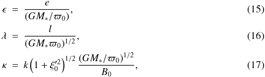with ϵ, λ, κ and the constant parameters that define the solution. With the help of Eqs. (10) − (17), and knowing that the Keplerian velocity is , one can find after some algebraic manipulation (see BP; Safier 1993) the following quartic equation for f(χ), $\mathit{T}\mathrm{-}{\mathit{f}}^{\mathrm{2}}\mathit{U}\mathrm{=}{\left[\frac{\mathrm{(}\mathit{\lambda }\mathrm{-}{\mathit{\xi }}^{\mathrm{2}}\mathrm{)}\mathit{m}}{\mathit{\xi }\mathrm{(}\mathrm{1}\mathrm{-}\mathit{m}\mathrm{)}}\right]}^{\mathrm{2}}\mathit{,}$(18)where $\begin{array}{ccc}\mathit{m}& \mathrm{\equiv }& \frac{\mathrm{4}\mathit{\pi \rho }\mathrm{(}{3}_{\mathit{\varpi }}^{\mathrm{2}}\mathrm{+}{3}_{\mathit{z}}^{\mathrm{2}}\mathrm{)}}{{\mathit{B}}_{\mathit{\varpi }}^{\mathrm{2}}\mathrm{+}{\mathit{B}}_{\mathit{z}}^{\mathrm{2}}}\mathit{,}\\ & \mathrm{=}& \mathit{\kappa \xi fJ}\end{array}$is the square of the (poloidal) Alfvén Mach number, and $\begin{array}{ccc}\mathit{T}& \mathrm{=}& {\mathit{\xi }}^{\mathrm{2}}\mathrm{+}\mathrm{2}\mathit{S}\mathrm{-}\mathrm{3}\mathit{,}\\ \mathit{S}& \mathrm{=}& \mathrm{(}{\mathit{\xi }}^{\mathrm{2}}\mathrm{+}{\mathit{\chi }}^{\mathrm{2}}{\mathrm{)}}^{\mathrm{-}\mathrm{1}\mathit{/}\mathrm{2}}\mathit{,}\\ \mathit{U}& \mathrm{=}& \mathrm{(}\mathrm{1}\mathrm{+}{\mathit{\xi }}^{\mathrm{\prime }\mathrm{2}}\mathrm{)}\mathit{,}\\ \mathit{J}& \mathrm{=}& \mathit{\xi }\mathrm{-}\mathit{\chi }{\mathit{\xi }}^{\mathrm{\prime }}\mathit{.}\end{array}$The flow trajectory solution is a self-similar solution that always crosses the disk at ξ = 1. If this self-similar solution, which is given by χ(ξ), is expanded into a polynomial function around the disk-crossing point using Taylor’s theorem, and we consider only the first three terms of the expansion, we will have a parabolic trajectory describing the outflow. This parabolic trajectory is given by $\mathit{\chi }\mathrm{\left(}\mathit{\xi }\mathrm{\right)}\mathrm{=}\mathit{a}{\mathit{\xi }}^{\mathrm{2}}\mathrm{+}\mathit{b\xi }\mathrm{+}\mathit{c,} \mathrm{with} \mathit{c}\mathrm{=}\mathrm{-}\mathrm{(}\mathit{a}\mathrm{+}\mathit{b}\mathrm{)}\mathit{.}$(25)This solution respects the launching condition, which states that the flow-launching angle ϑ₀ (see Fig. 1) should be less than ϑ_c = 60° for the material to accelerate magneto-centrifugally and be ejected as a wind from the disk. Equation (18) can be rewritten as a quartic equation for m, $\begin{array}{ccc}{\mathit{\xi }}^{\mathrm{2}}\mathit{V}{\mathit{m}}^{\mathrm{4}}\mathrm{-}\mathrm{2}{\mathit{\xi }}^{\mathrm{2}}\mathit{V}{\mathit{m}}^{\mathrm{3}}\mathrm{-}\mathrm{[}{\mathit{\xi }}^{\mathrm{2}}\mathrm{(}\mathit{T}\mathrm{-}\mathit{V}\mathrm{)}\mathrm{-}\mathrm{(}\mathit{\lambda }\mathrm{-}{\mathit{\xi }}^{\mathrm{2}}{\mathrm{)}}^{\mathrm{2}}\mathrm{]}{\mathit{m}}^{\mathrm{2}}& & \\ \mathrm{+}\mathrm{2}{\mathit{\xi }}^{\mathrm{2}}\mathit{Tm}\mathrm{+}{\mathit{\xi }}^{\mathrm{2}}\mathit{T}& \mathrm{=}& \end{array}$(26)$\mathrm{where} \mathit{V}\mathrm{=}\frac{\mathit{U}}{\mathrm{(}\mathit{\kappa \xi J}{\mathrm{)}}^{\mathrm{2}}}\mathrm{·}$(27)The solution of Eq. (26) gives four complex values of m for each pair of points (χ,ξ) inside the trajectory. The flow must reach super-Alfvénic speeds, for a strong self-generated toroidal field to appear, collimating the flux, and thus producing a jet (Blandford & Payne 1982). Of the four solutions of this quartic equation, there are only two real solutions that converge on one another at the Alfvén point, a sub-Alfvénic and a super-Alfvénic one. The sub-Alfvénic solution reaches the Alfvén speed and then the solution starts decreasing again, thus remaining a sub-Alfvénic solution before and after the Alfvén point. The same happens with the super-Alfvénic solution, which remains super-Alfvénic before and after the Alfvén point. The chosen solution must be a continuous real solution, and must also increase monotonically with χ, because the wind is constantly accelerated by the magnetic field. This solution is obtained by using the convergent sub-Alfvénic solution before the Alfvén radius, and then the super-Alfvénic one.

The launching condition imposes that , and it helps constrain the set of values of a, b, and c that can be used in Eq. (25). Then we can write ${\mathit{\xi }}_{\mathrm{0}}^{\mathrm{\prime }}\mathrm{=}\frac{\mathrm{1}}{\mathrm{2}\mathit{a}\mathrm{+}\mathit{b}}\gtrsim \cot {\mathit{\vartheta }}_{\mathrm{c}}\mathit{.}$(28)If the values of parameters κ and λ are also given, the flow can be fully described by the following equations: $\begin{array}{ccc}\mathit{f}& \mathrm{=}& \frac{\mathit{m}}{\mathit{\kappa \xi J}}\mathit{,}\\ {\mathit{f}}_{\mathrm{p}}& \mathrm{=}& \mathit{f}\mathrm{(}\mathrm{1}\mathrm{+}{\mathit{\xi }}^{\mathrm{\prime }\mathrm{2}}{\mathrm{)}}^{\mathrm{1}\mathit{/}\mathrm{2}}\mathit{,}\\ \mathit{g}& \mathrm{=}& \frac{{\mathit{\xi }}^{\mathrm{2}}\mathrm{-}\mathit{m\lambda }}{\mathit{\xi }\mathrm{(}\mathrm{1}\mathrm{-}\mathit{m}\mathrm{)}}\mathit{,}\\ \mathit{\eta }& \mathrm{=}& \frac{\mathrm{(}\mathit{\xi fJ}{\mathrm{)}}_{\mathrm{0}}}{\mathit{\xi fJ}}\mathrm{=}\frac{{\mathit{m}}_{\mathrm{0}}}{\mathit{m}}\mathit{,}\end{array}$where η and f_p are the self-similar dimensionless density and poloidal velocity, respectively. Knowing the gas density ρ, the poloidal velocity v_p, and the scaling laws, it can be shown that the mass loss rate Ṁ_loss is given by $\mathit{Ṁ}\mathrm{loss}\mathrm{=}\mathrm{2}\mathit{\pi }{\mathit{\rho }}_{\mathrm{0}}{\mathit{f}}_{\mathrm{p}\mathrm{0}}{\mathrm{(}\mathit{G}{\mathit{M}}_{\mathrm{\ast }}{{\mathit{\varpi }}_{\mathrm{0}}^{\mathrm{3}}}^{\mathrm{)}}}^{\mathrm{1}\mathit{/}\mathrm{2}}\ln \frac{{\mathit{r}}_{\mathrm{do}}}{{\mathit{r}}_{\mathrm{di}}}\mathit{,}$(33)where r_di and r_do are the inner and outer radii in the accreting disk that delimits the wind ejecting region (see Fig. 1). With this equation it is possible to calculate the value of ρ₀, which is necessary to produce a Ṁ_loss, when the wind leaves the disk between r_di and r_do.

The temperature structure we used inside the disk wind is similar to the one used in the magnetospheric accretion funnel. There are some studies about the temperature structure inside this region (Safier 1993; Panoglou et al. in prep.), and we are going to discuss them in Sect. 6.

The parameters used to calculate the self-similar wind solution were initially: a = 0.43, b =  − 0.20, λ = 30.0, κ = 0.03. These values of a and b were chosen to produce an intermediate disk-wind lauching angle ϑ₀ ≃ 33°, while for λ and θ these values are the same as the ones used by BP in their standard solution. We later changed some of these values to see how they influence our calculated Hα line profiles. The disk wind inner radius r_di = 3.01R_∗ is just slightly larger than r_mo, and we changed the value of the disk wind outer radius r_do from 5R_∗ to 30R_∗ to see how this affected the calculated profiles. To calculate ρ₀ we used a base value of Ṁ_loss = 10^-9   M_⊙yr^-1 = 0.1Ṁ_acc.

3. Radiative transfer model

In order to calculate the Hα line, it is necessary to know the population of at least levels 1 to 3 of the hydrogen atom. The model used for the hydrogen has three levels plus continuum. The high occupation number of the ground level, owing to the low temperatures in the studied region, leads to an optically thick intervening medium to the Lyman lines. Using this, it can be assumed that the fundamental level is in LTE. The other two levels plus ionization fraction were calculated with a two-level atom approximation (see Mihalas 1978, Chap. 11). The fundamental level population is used to better constrain the total number of atoms that are in levels 2 and 3, and is necessary to calculate the opacity due to H⁻ ion.

The line source function is calculated with the Sobolev approximation method (Rybicki & Hummer 1978; Hartmann et al. 1994). This method can be applied when the Doppler broadening is much larger than the thermal broadening inside the flow. Thus, an atom emitting a specific line transition only interacts with other atoms having a limited range of relative velocities, which occupy a small volume of the atmosphere. In the limit of high velocity gradients inside the flow, these regions with atoms that can interact with a given point additionally become very thin, and it can be assumed that the physical properties across this thin and small region remain constant. These small and thin regions are called “resonant surfaces”. Each point inside the atmosphere then only interacts with a few resonant surfaces, which simplifies the radiative transfer calculations a lot. The radiation field at each point can be described by the mean intensity $\mathit{J̅}\mathit{\nu }\mathrm{=}\mathrm{[}\mathrm{1}\mathrm{-}\mathit{\beta }\mathrm{(}{r}\mathrm{\left)}\mathrm{\right]}\mathit{S}\mathrm{\left(}{r}\mathrm{\right)}\mathrm{+}{\mathit{\beta }}_{\mathrm{c}}\mathrm{\left(}{r}\mathrm{\right)}{\mathit{I}}_{\mathrm{c}}\mathrm{+}\mathit{F}\mathrm{\left(}{r}\mathrm{\right)}\mathit{,}$(34)where β and β_c are the scape probabilities of local and continuum (stellar photosphere plus accretion shock, described by I_c) radiation, S is the local source function, and F is the non-local term, which takes into account only the contributions from the resonant surfaces. A more detailed description of each of these terms has been given in Hartmann et al. (1994).

Fig. 2 Temperature (left), poloidal velocity (middle), and density (right) profiles along streamlines inside the magnetosphere (top) and along streamlines inside the disk wind region (bottom). In all plots the x-axis represents the system cylindrical radius in units of stellar radii R∗. The maximum temperature inside the magnetosphere is Tmag,MAX ≃ 8000K, and inside the disk wind it is Twind,MAX ≃ 9000K. Only some of the streamlines are shown in the plots, and they are the same ones in the left, middle, and right plots.

For a particular line transition, the source function is given by ${\mathit{S}}_{\mathrm{ul}}\mathrm{=}\frac{\mathrm{2}\mathit{h}{\mathit{\nu }}_{\mathrm{ul}}^{\mathrm{3}}}{{\mathit{c}}^{\mathrm{2}}}{\left[\left(\frac{{\mathit{N}}_{\mathrm{l}}{\mathit{g}}_{\mathrm{u}}}{{\mathit{N}}_{\mathrm{u}}{\mathit{g}}_{\mathrm{l}}}\right)\mathrm{-}\mathrm{1}\right]}^{-1}\mathit{,}$(35)where N_l,N_u,g_l and g_u are the population and statistical weights of upper and lower levels of the transition respectively.

The flux is calculated as described by Muzerolle et al. (2001), where a ray-by-ray method was used. The disk coordinate system is rotated to a new coordinate system, given by the cartesian coordinates (P,Q,Z), in which the Z-axis coincides with the line of sight, and each ray is parallel to this axis. The specific intensity of each ray is given by ${\mathit{I}}_{\mathit{\nu }}\mathrm{=}{\mathit{I}}_{\mathrm{0}}{\mathrm{e}}^{\mathrm{-}{\mathit{\tau }}_{\mathrm{tot}}}\mathrm{+}{\mathrm{\int }}_{\mathit{\tau }\mathrm{(}\mathrm{-}\mathrm{\infty }\mathrm{)}}^{\mathit{\tau }\mathrm{\left(}{\mathit{Z}}_{\mathrm{0}}\mathrm{\right)}}{\mathit{S}}_{\mathit{\nu }}\mathrm{\left(}{\mathit{\tau }}^{\mathrm{\prime }}\mathrm{\right)}{\mathrm{e}}^{\mathrm{-}{\mathit{\tau }}^{\mathrm{\prime }}}\mathrm{d}{\mathit{\tau }}^{\mathrm{\prime }}\mathit{,}$(36)where I₀ is the incident intensity from the stellar photosphere or the accretion shock, when the rays hit the star, and is zero otherwise. S_ν(Z) is the source function at a point outside the stellar photosphere at frequency ν, and τ_tot is the total optical depth from the initial point, Z₀, to the observer ( − ∞), and τ( − ∞) = 0. Z₀ can be either the stellar surface, the opaque disk, or ∞. The optical depth from a point at Z to the observer is calculated as $\mathit{\tau }\mathrm{\left(}\mathit{Z}\mathrm{\right)}\mathrm{=}\mathrm{-}{\mathrm{\int }}_{\mathrm{-}\mathrm{\infty }}^{\mathit{Z}}\left[{\mathit{\chi }}_{\mathrm{c}}\mathrm{\left(}{\mathit{Z}}^{\mathrm{\prime }}\mathrm{\right)}\mathrm{+}{\mathit{\chi }}_{\mathrm{l}}\mathrm{\left(}{\mathit{Z}}^{\mathrm{\prime }}\mathrm{\right)}\right]\mathrm{d}{\mathit{Z}}^{\mathrm{\prime }}\mathit{,}$(37)in which χ_c and χ_l are the continuum and line opacities. The continuum opacity and emissivity contain the contributions from hydrogen bound-free and free-free emission, H^-, and electron scattering (see Mihalas 1978).

This model uses the Voigt profile as the profile of the emission or absorption lines that were modeled. Assuming a damping constant Γ, which controls the broadening mechanisms, a = Γ / 4πΔν_D, 3 = (ν − ν₀) / Δν_D, and Y = Δν / Δν_D, where Δν_D is the Doppler broadening due to thermal effects, and ν₀ the line center frequency, the Voigt function can be written as $\mathit{H}\mathrm{\left(}\mathit{a,}3\mathrm{\right)}\mathrm{\equiv }\frac{\mathit{a}}{\mathit{\pi }}{\mathrm{\int }}_{\mathrm{-}\mathrm{\infty }}^{\mathrm{\infty }}\frac{{\mathrm{e}}^{\mathrm{-}{\mathit{Y}}^{\mathrm{2}}}}{\mathrm{(}3\mathrm{-}\mathit{Y}{\mathrm{)}}^{\mathrm{2}}\mathrm{+}{\mathit{a}}^{\mathrm{2}}}\mathrm{d}\mathit{Y}\mathit{.}$(38)The line opacity is a function of the Voigt profile, and can be calculated by ${\mathit{\chi }}_{\mathrm{l}}\mathrm{=}\frac{{\mathit{\pi }}^{\mathrm{1}\mathit{/}\mathrm{2}}{\mathit{q}}_{\mathrm{e}}^{\mathrm{2}}}{{\mathit{m}}_{\mathrm{e}}\mathit{c}}{\mathit{f}}_{\mathit{ij}}{\mathit{n}}_{\mathit{j}}\left(\mathrm{1}\mathrm{-}\frac{{\mathit{g}}_{\mathit{j}}{\mathit{n}}_{\mathit{i}}}{{\mathit{g}}_{\mathit{i}}{\mathit{n}}_{\mathit{j}}}\right)\mathit{H}\mathrm{\left(}\mathit{a,}3\mathrm{\right)}\mathit{,}$(39)where f_ij, n_i, n_j, g_i, and g_j are the oscillator strength between level i and j, the populations of the ith and jth levels and the degeneracy of the ith and jth levels, respectively. The electron mass and charge are represented by m_e and q_e. The damping constant Γ contains the half-width terms for radiative, van der Waals, and Stark broadenings, and has been parameterized by Vernazza et al. (1973) as $\begin{array}{ccc}\mathrm{\Gamma }& \mathrm{=}& {\mathit{C}}_{\mathrm{rad}}\mathrm{+}{\mathit{C}}_{\mathrm{vdW}}\left(\frac{{\mathit{N}}_{\mathrm{HI}}}{{\mathrm{10}}^{\mathrm{16}}\mathrm{c}{\mathrm{m}}^{-3}}\right){\left(\frac{\mathit{T}}{\mathrm{5000}\mathrm{K}}\right)}^{\mathrm{0.3}}\\ & & \mathrm{+}{\mathit{C}}_{\mathrm{Stark}}{\left(\frac{{\mathit{N}}_{\mathrm{e}}}{{\mathrm{10}}^{\mathrm{12}}\mathrm{c}{\mathrm{m}}^{-3}}\right)}^{\mathrm{2}\mathit{/}\mathrm{3}}\mathit{,}\end{array}$(40)where C_rad, C_vdW and C_Stark are the radiative, van der Waals, and Stark half-widths, respectively, in Å, N_HI is the number density of neutral hydrogen, and N_e the number density of electrons. Radiative and Stark broadening mechanisms are the most important for the Hα line in our modeled environment. Stark broadening is significant (or dominant) inside the magnetosphere, due to the high electron densities in this region. However, inside the disk wind, N_e becomes very low, and Stark broadening becomes very weak compared to radiative broadening. These effects are small compared to the thermal broadening inside the studied region.

The total emerging power in the line of sight for each frequency (P_ν) is calculated by integrating the intensity I_ν of each ray over the projected area dPdQ. The emerging power in the line of sight depends only on the direction. Thus, instead of using flux in our plots, which also depends on the distance from the source, we present our profiles as power plots.

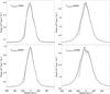Fig. 3 Hα profiles for the default case with values of Tmag,MAX ranging from 7500 K to 10 000 K and values of Twind,MAX ranging from 7000 K to 10 000 K. The maximum magnetospheric temperature Tmag,MAX in each plot is the same, and each different line represents a different maximum disk wind temperature Twind,MAX: 7000 K (black solid line), 8000 K (grey solid line), 9000 K (black dotted line) and 10 000 K (black dashed line). The dash-dotted dark grey lines in each plot show the profiles calculated with only the magnetospheric component (no disk wind). The black and grey solid lines completely overlap each other.

4. Results

As a starting point, we used the parameters summarized in Table 1 to calculate Hα line profiles. We used a default inclination i = 55° in these calculations. For Ṁ_loss, r_di and r_do as given by Table 1, we calculated with Eq. (33) a fiducial density ρ₀ = 4.7 × 10^-12gcm^-3. The set of maximum temperatures inside the magnetosphere and the disk wind region employed in the model ranges from 6000K to 10000K, as used by Muzerolle et al. (2001). As an example, Fig. 2 shows the temperature profiles for the case when the maximum temperature inside the magnetosphere, T_mag,MAX ≃ 8000K, and the maximum temperature inside the disk wind, T_wind,MAX ≃ 9000K. Figure 2 shows some of the streamlines to illustrate the temperature behavior along the flow lines. Inside the magnetosphere, we can see that there is a temperature maximum midway between the disk and the star, and the maximum temperature is higher for streamlines starting farther away from the star. Inside the disk wind it is the opposite, the maximum temperature along a flux line starts higher near the star, and decays with receding launching point from the star. Also for the nearest flux lines the temperature reaches a maximum and then starts falling inside the disk wind, and for more extended launching regions the temperature seems to reach a plateau and then remains constant along the line. The right plots in Fig. 2 show the density profiles along the streamlines inside the magnetosphere and disk wind. The temperature law used assumes that , where N_H is the total number density of hydrogen, which explains the similarities between the temperature and density profiles. Each streamline is composed of 40 grid points. These lines reach a maximum height of 32R_∗ in the disk wind.

Figure 2 also shows the poloidal velocity profiles inside the magnetosphere and the disk wind. Inside the magnetosphere, the velocity reaches its maximum when the flow hits the stellar surface, and it is faster for lines that start farther away from the star. Inside the disk wind, the outflow speed increases continuously and monotonically, as required by the BP solution, and this acceleration is fastest for the innermost streamlines. We can see that the terminal speeds of each streamline inside the magnetosphere have a very low dispersion and reach values between  ≃ 230kms^-1 and  ≃ 260kms^-1. Inside the disk wind, this velocity dispersion is much higher, with the flow inside the innermost streamline reaching speeds faster than 250kms^-1, while the flow inside the outermost line shown in Fig. 2 – which is not identical with the outermost line we have used in our default case – is reaching maximum speeds around  ≃ 70kms^-1. Note that even considering a thin disk, our disk wind and magnetosphere solutions do not start at z = 0, and the first point in the disk wind streamlines is always at some height above the accretion disk, which is the reason why the poloidal velocities are not starting from zero.

The Hα line profiles have a clear dependence on the temperature structures of the magnetosphere and the disk wind region. Figure 3 shows plots for different values of T_mag,MAX, and each plot shows profiles for different values of T_wind,MAX, which are shown as different lines. The black solid lines are the profiles with only the magnetosphere’s contribution. One can see that in the default case, most of the Hα flux comes from the magnetospheric region, which is highly dependent on the magnetospheric temperature. In all plots there is no noticeable difference between T_wind,MAX ≃ 7000K (black solid line) and T_wind,MAX ≃ 8000K (grey solid line), and the disk wind contribution in these cases is very small, only appearing around the line center as an added contribution to the total flux, while there are no visible contributions in the line wings. When T_wind,MAX is around 9000 K, a small blue absorption component starts appearing, which becomes stronger as both the magnetospheric and disk wind temperatures increase. The same happens for the added disk wind contribution to the flux around the line center.

Figure 4 shows the variation of the Hα line with the mass accretion rate (Ṁ_acc). In all plots, the mass loss rate was kept at 10% of the mass accretion rate, and the maximum temperature inside the magnetospheric accretion funnel was around 9000 K. For Ṁ_acc = 10^-9   M_⊙yr^-1, the plot shows that the line does not change much when the disk wind temperature varies from 6000 K to 10 000 K, because all lines that consider the disk wind contribution are overlapping. There is an overall small disk wind contribution to the flux that is stronger around the line center. In this case, the disk wind contribution to the line center increases slightly as the temperature becomes hotter than 10 000 K. If the temperature becomes much higher than that, most of the hydrogen will become ionized and no significant absorption in Hα is to be expected. When the mass accretion rate rises to Ṁ_acc = 10^-8   M_⊙yr^-1, the Hα flux becomes stronger, and the line broader. There is no blue-ward absorption feature until the temperature inside the disk wind reaches about 9000 K (see Fig. 3), after that the blue-shifted absorption feature becomes deeper as the temperature rises. Finally, for a system where Ṁ_acc = 10^-7   M_⊙yr^-1, the line becomes much broader, and even for maximum temperatures inside the disk wind below 8000 K, a blue-shifted absorption component can be seen. This absorption becomes deeper with increasing disk wind temperature. In this last case, the disk wind contribution to the flux is on the same order of magnitude as the contribution from the magnetosphere, which does not happen for lower accretion rates.

When ρ₀ is kept constant and the outer wind radius varies, then Ṁ_loss also changes. When that is done, it is also possible to discover the region inside the disk wind which contributes the most to the line flux. Figure 5 shows how the line changes with r_do, while ρ₀ remains constant. Where Ṁ_acc = 10^-8   M_⊙yr^-1 (Fig. 5a), we can see that the line profiles for r_do = 30.0   R_∗ and r_do = 10.0   R_∗ are almost at exactly the same place, which means that in this case most of the contribution of the disk wind comes from the wind that is launched at r < 10   R_∗. And as r_do becomes even smaller, the blue-shifted absorption feature begins to become weaker and the line peak starts to decrease, until the only contributing factor to the line profile is the magnetospheric one. For Ṁ_acc = 10^-7   M_⊙yr^-1 (Fig. 5b), a similar behavior can be seen, but in this case the plots show the loss of a substantial amount of flux when r_do goes from r_do = 30.0   R_∗ to r_do = 10.0R_∗, an effect mostly seen around the line peak. The same happens at the blue-shifted absorption feature, which begins to weaken when r_do ≲ 15.0   R_∗, and weakens faster as r_do decreases. In both cases, most of the Hα flux contribution from the wind comes from the region where the densities and temperatures are the highest, and this region extends farther away from the star for higher mass loss rates, as expected. But even for high values of Ṁ_loss, all absorption comes from the gas that is launched from the disk in a radius of at most some tens of R_∗ from the star. In both cases, it seems that a substantial part of the disk wind contribution to the Hα flux around the line center comes from a region very near the inner edge of the wind, because we still can see a sizeable disk wind contribution around the line center even when r_do = 3.5   R_∗.

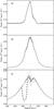Fig. 4 Hα profiles for different values of Ṁacc: a) 10-9   M⊙yr-1, b) 10-8   M⊙yr-1 and c) 10-7   M⊙yr-1. The maximum magnetospheric temperature used is Tmag,MAX ≃ 9000 K, and the values used for Twind,MAX are 6000 K (black thin solid line), 8000 K (dark grey thick dashed line) and 10 000 K (light grey thin dashed line). The light grey thin solid lines are the profiles where only the magnetosphere is considered. In all cases, the Ṁloss ≈ 0.1   Ṁacc.

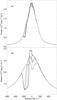Fig. 5 Hα profiles for a) Ṁacc = 10-8   M⊙yr-1, and b) Ṁacc = 10-7   M⊙yr-1, with Tmag,MAX = 9000 K and Twind,MAX = 10000 K. In all plots the value of ρ0 is kept constant at a value which makes Ṁloss ≈ 0.1   Ṁacc, when rdo = 30.0   R∗. The black thin solid lines are the line profiles with only the magnetosphere; the thick darkgrey solid lines are the line profiles when magnetosphere and disk wind are considered and rdo = 30.0   R∗. The other curves show the line profiles when rdo = 10.0   R∗ (thin black dashed lines), rdo = 5.0   R∗ (thin black dotted line), rdo = 4.0   R∗ (dark grey thin dashed line) and rdo = 3.5   R∗ (light grey thin solid line).

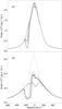Fig. 6 Hα profiles as in Fig. 5, but now the density ρ0 is varied to keep the mass loss rate at 0.1   Ṁacc, while the disk wind outer radius rdo changes from 30.0   R∗ to 5.0   R∗, and each line represents a different rdo and a different ρ0. In a), rdo = 30.0   R∗ and ρ0 = 4.71 × 10-12   gcm-3 (dark grey thick solid line), rdo = 20.0   R∗ and ρ0 = 5.72 × 10-12   gcm-3 (black thin dashed line), rdo = 10.0   R∗ and ρ0 = 9.02 × 10-12   gcm-3 (black thin dotted line), rdo = 7.5   R∗ and ρ0 = 1.19 × 10-11   gcm-3 (dark grey thin dashed line), rdo = 5.0   R∗ and ρ0 = 2.13 × 10-11   gcm-3 (light grey thin solid line). In b), the lines have the same value of rdo, but their ρ0 are 10 times higher than in a). The black thin line represents the line profile with only the magnetospheric component.

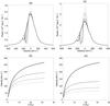Fig. 7 Hα profiles when Ṁacc = 10-8   M⊙yr-1 with Tmag,MAX = 9000 K and Twind,MAX = 10000 K. Left panels show a) the Hα profile for different values of λ, and b) the corresponding poloidal velocity profiles for the innermost line of the outflow. The lines in the left panels are: λ = 30 (solid line), λ = 40 (dashed line), λ = 50 (dash-dotted line) and λ = 60 (dotted line). The right panels show c) the Hα profile for different values of κ, and d) the corresponding poloidal velocity profiles for the innermost streamline of the outflow. The lines in the right panel are: κ = 0.03 (solid line), κ = 0.06 (dashed line), κ = 0.09 (dash-dotted line) and κ = 0.12 (dotted line). The mass loss rate is kept constant at 0.1   Ṁacc.

If instead Ṁ_loss is kept constant while both r_do and ρ₀ change, it is possible to infer how the size of the disk wind affects the Hα line as shown in Fig. 6. In the default case (Fig. 6a, Ṁ_acc = 10^-8   M_⊙yr^-1), with T_mag,MAX ≃ 9000 K, and T_wind,MAX ≃ 10000 K, and changing r_do from 30   R_∗ to 5   R_∗ while also changing the densities to keep the mass loss rate constant, there are almost no variations around the line peak, as all the profiles with the disk wind contribution overlap in this region. Some differences can be seen at the blue-shifted absorption component, which becomes deeper as the disk wind size decreases and the density increases. For a higher mass loss rate (Fig. 6b, Ṁ_acc = 10^-7   M_⊙yr^-1), the line peak decreases when r_do goes from 30   R_∗ to 20   R_∗, while the absorption feature barely changes. But as r_do diminishes even further, the line flux as a whole begins to become much stronger again, while the absorption apparently becomes lower. Thus, it seems for moderate values of Ṁ_acc that the size of the disk-wind launching region does not have a great influence on the Hα line flux, with only some small differences in the depth and width of the line profile absorption feature. However, for higher Ṁ_acc, the profiles start to vary rapidly when r_do < 20.0   R_∗, and the line flux increases faster as r_do decreases. In spite of these differences, we noticed that in both cases this increase in the Hα flux only becomes important when ρ₀ ≳ 10^-10   gcm^-3, which happens for r_do ≲ 7.5   R_∗ when Ṁ_acc = 10^-7   M_⊙yr^-1, and for r_do ≲ 4   R_∗, which is out of the plot range in Fig. 6a, when Ṁ_acc = 10^-8   M_⊙yr^-1. This indicates that the densities inside the disk wind region are very important to define the overall Hα line shape, if ρ₀ ≳ 10^-10   gcm^-3. Still, if ρ₀ is smaller, its effect, if any, is smaller and is mostly present around the absorption feature.

So far we used λ = 30 and κ = 0.03 in all above mentioned cases. The λ parameter is the dimensionless angular momentum, and together with ϵ, the dimensionless specific energy, is constant along a streamline. Equations (8), (9), (15), and (16) show that a variation in λ will produce a change in the velocities along the streamline. This change in λ will also produce a different disk wind solution, and consequently it is necessary to change the value of ρ₀ to keep the mass loss rate the same. The effect of λ in the line profile can be seen in Fig. 7a for the default model parameters and a constant mass loss rate. It shows that as the value of λ is increased, the absorption feature becomes deeper and closer to the line center, which means a slower disk wind, and also an increase in the line flux around its center. Figure 7b illustrates this behavior and shows how the poloidal velocity profile changes when the value of λ is varied.

The Hα flux varies in a similar manner when the value of κ, the dimensionless mass flux to magnetic flux ratio, is changed, which is illustrated by Fig. 7c. As κ increases, the mass flow becomes slower (see Eqs. (11) and (29)), and the absorption feature also comes closer to the line center. The higher the value of κ, the deeper is the blue-shifted absorption and the stronger is the flux at the line center, similar to the case when λ varies. There is also a large variation of the poloidal speed inside the flux when κ changes, which is shown by Fig. 7d. Both Figs. 7b and d confirm the behavior seen in Figs. 7a and c. An increase in the values of λ or κ decreases the poloidal velocities and the velocity dispersion inside the disk wind, causing the absorption feature to approach the line center. The lower velocity dispersion causes the line opacity to be raised around the absorption feature, which strengthens it. This increase in λ or κ also requires an increase in the densities inside the outflow, if the mass loss rate is to be kept constant, and this effect also enhances the absorption feature and the line flux around its center.

The disk-wind launching angle ϑ₀ also produces a variation in the Hα line profile. To change ϑ₀, it is necessary to change the coefficients a and b of Eq. (25). Here, b is kept constant, and only the coefficient a is varied. A change in the coefficients a and b produces another disk wind solution, and then it is necessary to recalculate ρ₀ to hold the mass loss rate constant. In Fig. 8, ϑ₀ varies from 14.6° to 55.6°, which is almost at the launching condition limit, and the value of a used in each case is indicated in the caption. Figure 8 shows that the absorption feature moves closer to the line center as the launching angle steepens. Again, as with the cases when we changed κ and λ, a variation in the launching angle produces a variation in the launching speed, and this variation is shown at the bottom panel of Fig. 8. The launching speed is slower for higher launching angles, and this increases the densities inside the wind. When ϑ₀ = 14.6°, the case with the fastest launching speed, there is no noticeable difference between the profile with the disk wind contribution and the one with only the magnetosphere contribution. This is also the case with the lowest disk wind densities, which are so low that there is no visible absorption, and just a small disk wind contribution around the center of the line. The case with ϑ₀ = 33.4° is the default case used in all the prior plots. When the launching angle becomes steeper, the disk wind becomes denser, and then we have a larger disk wind contribution to the profile and a deeper blue-shifted absorption feature. Again, the lower velocity dispersion inside the disk wind also helps to enhance the disk wind contribution to the Hα when the launching angle becomes steeper.

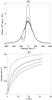Fig. 8 Hα profiles a) and poloidal velocity profiles for the innermost disk wind streamline b) for different values of the launching angle ϑ0. The lines are: ϑ0 = 14.6° and a = 0.23 (gray solid line), ϑ0 = 33.4° and a = 0.43 (dot-dot-dot-dashed line), ϑ0 = 46.7° and a = 0.63 (dot-dashed line), ϑ0 = 55.6° and a = 0.83 (dashed line). The full black line in a) represents the profile with only the magnetosphere. In all the plots, b =  − 0.20, Ṁacc = 10-8   M⊙yr-1, Tmag,MAX = 9000K and Twind,MAX = 10000K.

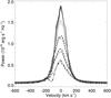Fig. 9 Hα profiles with different star-disk system inclinations, i, Ṁacc = 10-8   M⊙yr-1, Tmag,MAX = 8000 K and Twind,MAX = 10000 K. For each i, there is a plot showing the total profile with both magnetosphere and disk wind contributions (black line), and a profile with only the magnetosphere contribution (gray line). The lines are: i = 15° (solid), i = 30° (dotted), i = 45° (dashed), i = 60° (dot-dashed), and i = 75° (dot-dot-dot-dashed).

One of the most important factors defining the line profiles is the system inclination from the line of sight, i. Figure 9 shows how the Hα line changes with i, when Ṁ_acc = 10^-8   M_⊙yr^-1, T_mag,MAX = 8000 K and T_wind,MAX = 10000 K. It is obvious that the profile intensity is stronger for lower inclinations, and this has a series of reasons. First, because the solid angle containing the studied region is larger for lower values of i, and this leads to a higher integrated line flux over the solid angle. The opacity inside the accretion columns is lower if we are looking at them at a lower inclination angle, and then we can see deeper inside, which increases the line flux. Finally, the shadowing by the opaque accretion disk and by the star makes the lower accretion columns less visible with a higher i, which also decreases the total flux. The Hα photon that leaves the magnetosphere or the star crosses an increasingly larger portion of the outflow as i becomes steeper, which strengthens the blue-shifted absorption feature. Another effect that happens when the inclination changes is that the disk wind velocities projected on the line of sight decrease as the inclination becomes steeper, and make the blue-shifted absorption feature approach the line center, as is illustrated by Fig. 9. The projected velocities increase until i reaches a certain angle, which depends on the disk wind geometry, and then as the inclination keeps increasing, the projected velocities start to decrease again. The disk wind contribution to the red part of the Hα profile becomes weaker as i decreases, because there is barely a contribution to the red part of the profile when i = 15°, while this red-shifted contribution seems to be much stronger when i = 60° and i = 75°. If the disk-wind launching angle, ϑ₀, is smaller than i, part of the disk wind flux will be red-shifted. This red-shifted region inside the outflow becomes larger as i increases, and this increases the red-ward disk wind contribution to the total line flux.

The system inclination also affects the continuum level in the line profile. At lower inclinations, the upper accretion ring, with its much higher temperature than the stellar photosphere is much more visible than at higher inclinations. Moreover, at higher inclinations most of the stellar photosphere is covered by the accretion columns. Then, in a system with low inclination, the continuum level is expected to be significantly stronger than in systems with a high inclination. Analyzing Figs. 4 and 9 together, we can see that this variation in the continuum is really significant. Figure 4a shows exactly where the continuum level is when i = 55°, and comparing it with Fig. 9, it is possible to note an increase between 30% and 50% in the continuum level when the inclination changes from 75° to 15°.

Many of the line profiles calculated by our model have some irregular features at their cores. These features become more irregular as the mass accretion rate and temperature increase. A very high line optical depth inside the magnetosphere due to the increased density can create some self-absorption in the accretion funnel, resulting in these features. Also, the Sobolev approximation breakes down for projected velocities near the rest speed. Under SA, the optical depth between two points is inversely proportional to the projected velocity gradient between these points. Thus, in subsonic regions like in the base of the disk wind, or in regions where the velocity gradient is low, SA predicts a opacity that is much higher than the actual one, which creates the irregularities seen near the line center that are present in some of the profiles. If instead we do not assume SA, our profiles would be slightly more intense and smoother around the line center. However, the calculation time would increase considerably.

5. Discussion

The analysis of our results indicates a clear dependence of the Hα line on the densities and temperatures inside the disk wind region. The bulk of the flux comes mostly from the magnetospheric component for standard parameter values, but the disk wind component becomes more important as the mass accretion rate rises, and as the disk wind temperature and densities become higher, too. For very low mass loss rates (Ṁ_loss = 10^-10   M_⊙yr^-1) and disk wind temperatures below 10 000 K, there is a slight disk wind component that helps the flux at the center of the line only minimally. No absorption component can be seen even for temperatures in the wind as high as 17000K, which is expected because in such a hot environment most of the hydrogen will be ionized. Thus, only the cooler parts of the disk wind where the gas is more rarified would be able to produce a minimal contribution to the Hα flux. The fiducial density in this case is ρ₀ = 4.7 × 10^-13   gcm^-3, when the disk-wind launching region covers a ring between 3.0   R_∗ ( ≈ 0.03 AU) and 30.0   R_∗ ( ≈ 0.3 AU). Some studies suggest that the outer launching radius for the atomic component of the disk wind is between 0.2 − 3 AU (Anderson et al. 2003; Pesenti et al. 2004; Ferreira et al. 2006; Ray et al. 2007), which is much larger that the values of the disk wind outer radius used here. This means that the densities inside the disk wind should be even lower than the values we used, but as the fiducial density falls logarithmically with r_do (Eq. (33)), the density would not be much lower. The density for low mass loss rate (10^-10   M_⊙yr^-1) is already so low that a further decrease in its value would not produce a significant change in the disk wind contribution to the profile. However, the decreased density would create an environment where a blue-shifted absorption in the Hα line would be much more difficult to be formed. So, for Ṁ_acc < 10^-9   M_⊙yr^-1, the disk wind contribution to the total Hα flux is negligible, which is consistent with observations (e.g. Muzerolle et al. 2003, 2005). A blue-shifted absorption in this case is meant to appear if the disk wind outer radius is much closer to the star than the observational studies suggest.

For cases with higher values of Ṁ_acc, and thus higher densities inside the disk wind region, it is possible to see a transition temperature, below which no blue-shifted absorption feature can be observed (Fig. 4). This temperature is between 8000 K and 9000 K when Ṁ_acc = 10^-8   M_⊙yr^-1, between 6000 K and 7000 K when Ṁ_acc = 10^-7   M_⊙yr^-1, and it might be even lower than 6000 K for cases with very high accretion rates (Ṁ_acc > 10^-7   M_⊙yr^-1). This transition temperature will directly depend on the mass densities inside the disk wind. Figure 4 also shows that the overall added disk wind contribution to the flux becomes more important as the accretion rate becomes stronger, due to a denser disk wind. It is then possible to imagine some conditions that would make the disk wind contribution to the Hα flux even surpass the magnetospheric contribution: a very high mass accretion rate (Ṁ_acc > 10^-7   M_⊙yr^-1), or a very large region inside the disk wind with temperatures  ~ 9000 K, or r_do ≪ 30   R_∗, or even a combination of all these conditions.

The density inside the outflow alone is a very important factor in the determination of the disk wind contribution to the Hα total flux. The blue-shifted absorption feature that can be seen in many of the profiles is directly affected by the disk wind densities, which change their depth and width as ρ₀ changes. Yet, the other parts of the line profile seem barely to be affected by the same variation in ρ₀, if ρ₀ ≲ 10^-10   gcm^-3, and the mass loss rate and the disk wind solution remain the same. But when ρ₀ ≳ 10^-10   gcm^-3, the variation in the line profile begins to adopt another behavior, and the line as a whole becomes dependent on the disk wind densities, which becomes stronger as ρ₀ increases even more. Densities higher than that transition value would only occur, again, if the mass loss rates are very high, or if r_do is just a few stellar radii above the stellar surface in the case of moderate to high mass accretion rates.

Another interesting result that we obtained shows that even if the disk wind outer radius r_do is tens of stellar radii above the stellar surface, most of the disk wind contribution to the Hα flux around line center comes from a region very near the disk wind inner edge. This happens because of the higher densities and temperatures in the inner disk wind region if compared to its outer regions, which makes the inner disk wind contribution much more important to the overall Hα flux than the other regions. This result suggests that the more energetic Balmer lines should be formed in a region narrower than the one where the Hα line is formed, but a region that also starts at r_di. However, the blue-shifted absorption feature seems to be formed in a region that goes from the inner edge to an intermediate region inside the disk wind, which is  < 30   R_∗, in the studied cases (see Fig. 5).

According to BP, not all values of κ and λ are capable of producing super-Alfvénic flows at infinity, a condition that enables the collimation of the disk wind and the formation of a jet. The condition necessary for a super-Alfvénic flow is that κλ(2λ − 3)^1 / 2 > 1, which is true in all plots in this paper. Another condition necessary for a solution is that it must be a real one and the velocities inside the flux must increase monotonically, which more constrains the set of values of κ, λ, and ϑ, which can produce a physical solution. The BP solution is a “cold” wind solution, where the thermal effects are neglected and only the magneto-centrifugal acceleration is necessary to produce the outflow from the disk. The results presented here show that the disk wind contribution to the Hα flux dependents very much on the disk wind parameters used to calculate its self-similar solutions. By changing the values of κ, λ, and ϑ₀, we change the self-similar solutions of the problem. Thus, changing the velocities and densities inside the disk wind, leads to a displacement of the blue-shifted absorption component and a variation, more visible around the rest velocity, in the overall disk wind contribution to the flux. For a “warm” disk wind solution, with strong heating mechanisms acting upon the accretion disk surface, and producing an enhanced mass loading on the disk wind, a much lower λ ≈ 2 − 20 would be necessary (Casse & Ferreira 2000). We worked only with the “cold” disk wind solution, but it is possible to use a “warm” solution, if we find the correct set of values for λ and κ.

Figure 9 shows a dependence of the line profile with inclination i similar to that found by KHS using their disk-wind-magnetosphere hybrid model. In both models, the Hα line profile intensity decreases as i increases, and so does the line equivalent width (EW). These results contradict the result from Appenzeller et al. (2005), who have shown that the observed Hα from CTTS increase their EW as the inclination angle increases. A solution to that problem, as shown by KHS, is to add a stellar wind contribution to the models, because that would increase the line EW at lower inclination. A larger sample than the 12 CTTS set used by Appenzeller et al. (2005) should also be investigated before more definite conclusions are drawn. However, there is a great difference between the blue-shifted absorption position in our model and in the KHS model. In their model, the blue-shifted absorption position is around the line center, while in ours it is at a much higher velocity. This difference arises from the different disk wind geometry used in both models. Kurosawa et al. (2006) used straight lines arising from the same source point to model their disk wind streamlines, which results in the innermost streamlines having a higher launching angle and thus lower projected velocity along the line of sight in that region when i is large. Instead we use parabolic streamlines, and these lines have a higher projected velocity in our default case along the line of sight, displacing our absorption feature to higher velocities.

In both models it is common to have the magnetospheric contribution as the major contribution to the Hα flux, with a much smaller disk wind contribution. In a few of the profiles calculated by KHS, the disk wind contribution is far more intense than the magnetospheric contribution. With their disk-wind-magnetosphere hybrid model and using Ṁ_acc = 10^-7   M_⊙yr^-1, T_wind = 9000   K and β = 2.0, KHS have obtained a disk wind contribution to the Hα flux one order of magnitude higher than the magnetospheric contribution. In their model, β is the wind acceleration parameter, and the higher its value, the slower is the wind accelerated, which leads to a denser and more slowly accelerated outflow in some regions of the disk wind. Kurosawa et al. (2006) used an isothermal disk wind. A large acceleration parameter (β = 2.0), leading to a large region with a high density, which is coupled with an isothermal disk wind at high temperature (T_wind = 9000 K), would then lead to a very intense disk wind contribution. However, the β = 2.0 value of their model is an extreme condition. For our model to produce a disk wind contribution as high as in that extreme case, we would also need very extreme conditions, although due to the differences between the models, these conditions should present themselves as a different set of parameters. The modified BP disk wind formulation used in our model produces a very different disk wind solution than that used by KHS, the disk wind acceleration in our solution is dependent on λ, κ and ϑ₀ parameters (see Figs. 7b, d and 8). We also use a very different temperature law (see Fig. 2), which is not isothermal, and a different geometric configuration. It is however also possible to obtain a very intense disk wind contribution with the correct set of parameters, which corresponds as in KHS to a very dense and hot disk wind solution.

Comparing our results with the classification scheme proposed by Reipurth et al. (1996), we can see for the Hα emission lines of TTS and Herbig Ae/Be stars that most of the profiles in this paper can be classified as Type I (profiles symmetric around their line center) or Type III-B (profiles with a blue secondary peak that is less than half the strength of the primary peak). These two types of Hα profiles correspond to almost 60% of the observed profiles in the Reipurth et al. (1996) sample of 43 CTTS. Figure 4a also shows a profile that can be classified as Type IV-R. We have not tried to reproduce all types of profiles in the classification scheme of Reipurth et al. (1996), but with the correct set o parameters in our model, it should be possible to reproduce them. Even with our different assumptions, our model and KHS model also produce many similar results, and both models can reproduce many of the observed types of Hα line profiles of CTTS, but the conditions necessary for both models to reproduce each type of profile should be different.

We are working with a very simple model for the hydrogen atom, with only the three first levels plus continuum. A better atomic model, which takes into consideration more levels of the hydrogen atom, would give us more realistic line profiles and better constraints for the formation of the Hα line, and would allow us to make similar studies using other hydrogen lines. The assumption that the hydrogen ground level is in LTE due to the very high optical depth to the Lyman lines is a very good approximation inside the accretion funnels, and even in the densest parts of the disk wind, but it may not be applicable in the more rarified regions of the disk wind. In those regions, the intervening medium will be more transparent to the Lyman lines, thus making the LTE assumption for the ground level invalid. Using a more realistic atom in non-LTE would lower the population of the ground level, and in turn the populations of levels 2 and 3 would increase. The line source function [Eq. (35)] depends on the ratio between the populations of the upper and lower levels, so, if the population of the level 3 increases more than the population of the level 2, the Hα emission will increase, otherwise the line opacity will increase. In any case, this will increase the disk wind effects upon the Hα line, thus making the disk wind contribution in cases with low to very low accretion rates important to the overall profile. The real contribution will depend on each case and is hard to predict. Still, even with all the assumptions used in our simple model, we could study how each of the disk wind parameters affects the formation of the Hα line on CTTS. Moreover, the general behavior we found might still hold true for a better atomic model, only giving us different transition and limiting values.

It is necessary to better understand the temperature structures inside the magnetosphere, and inside the disk wind, if we wish to produce more precise line profiles. A study about the temperature structure inside the disk wind done by Safier (1993) found that the temperature inside the disk wind starts very low ( ≲ 1000 K), for lines starting in the inner 1AU of the disk, then reaches a maximum temperature on the order of 10⁴ K, and remains isothermal on scales of  ~ 100–1000 AU. That temperature law is very different from the one used in our models, and it would produce very different profiles than the ones we have calculated here, because the denser parts of the outflow, in Safier (1993), have a much lower temperature than in our model. But Safier (1993) only considered atomic gas when calculating the ionization fraction, and did not consider H₂ destruction by stellar FUV photons, coronal X-rays, or endothermic reactions with O and OH. A new thermo-chemical study about the disk wind in Class 0, Class I, and Class II objects is prepared by Panoglou et al. (in prep.), where they address this problem, adding all the missing factors not present in Safier (1993) and also including an extended network of 134 chemical species. Their results produce a temperature profile that is similar to the ones we used here, but which is scaled to lower temperatures. Nevertheless, the innermost streamline they show in their plots is at 0.29 AU, which is around 30   R_∗ in our model and their temperature seems to increase as it nears the star. This strengthens the conviction that the temperature structure used in our model is still a good approximation.

The parameter that defines the temperature structure inside the magnetosphere and inside the disk wind is the Λ parameter, defined by Hartmann et al. (1982), and it represents the radiative loss function. It is then possible to use Λ to infer the radiative energy flux that leaves the disk wind in our models, and even in the most extreme scenarios, the radiative losses in the disk wind are much lower than the energy generated by the accretion process. Our model is consequently not violating any energetic constraints.

In a following paper we plan to use our model to reproduce the observed Hα lines of a set of classical T Tauri stars exhibiting different characteristics. After that, we plan to improve the atomic model to obtain more realistic line profiles of a large variety of hydrogen lines.

6. Conclusions

We developed a model with an axisymmetric dipolar magnetic field in the magnetosphere that was firstly proposed by Hartmann et al. (1994), and then improved by Muzerolle et al. (1998, 2001), adding a self-similar disk wind component as proposed by Blandford & Payne (1982), and a simple hydrogen atom with only three levels plus continuum. We have investigated which are the most important factors that influence the Hα line in a CTTS, and which region in the CTTS environment is the most important for the formation of this line. We have reached the following conclusions:

• The bulk of the Hα line flux comes from the magnetosphere for CTTS with moderate (Ṁ_acc ≈ 10^-8   M_⊙yr^-1) to low mass accretion rates (Ṁ_acc ≲ 10^-9   M_⊙yr^-1). For CTTS with high mass accretion rates (Ṁ_acc ≳ 10^-7   M_⊙yr^-1), the disk wind contribution is around the same order of magnitude as the magnetospheric contribution. In very extreme scenarios, it is possible to make the disk wind contribution much more important than the magnetosphere’s contribution.

• There is a transition value of T_wind,MAX below which no blue-shifted absorption feature can be seen in the Hα line profile. This transition temperature depends on the mass loss rate, and is lower for higher values of Ṁ_loss. This transition value can reach from T_wind,MAX ≲ 6000 K for CTTS with very high mass loss rates (Ṁ_loss > 10^-8   M_⊙yr^-1), to T_wind,MAX ~ 9000 K for stars with moderate mass loss rates (Ṁ_loss ~ 10^-9   M_⊙yr^-1). This transition temperature must not be much higher than 10 000 K, otherwise most of the hydrogen will be ionized. The disk wind in CTTS with Ṁ_loss < 10^-10   M_⊙yr^-1 should not produce any blue-shifted absorption in Hα. The other disk wind parameters that affect the outflow density can also change the value of this transition T_wind,MAX.

• Most of the disk wind contribution to the Hα flux comes from the inner regions of the disk wind, and the blue-shifted absorption feature that can be seen in most of the observed profiles is also formed around the same region. For Ṁ_loss ≤ 10^-8   M_⊙yr^-1, most of the disk wind Hα flux comes from the outflow launched from r ≲ 20   R_∗ in the disk. This region is larger for higher mass loss rates. The size of this region depends on the mass loss rate, density, and temperatures inside the disk wind.

• The blue-shifted absorption component dependents very much on the size of the disk wind, but except for this feature, the disk wind contribution to the Hα line barely changes if the Ṁ_loss is kept constant while r_do changes. In a scenario with a small r_do, the disk wind density might surpass a certain limiting value (ρ₀ ≳ 10^-10   gcm^-3), making the disk wind contribution to the profile very strong, even the main contribution to the profile in more extreme cases. This value for ρ₀ should change if we instead use a more realistic hydrogen atom.

• The disk wind parameters that define its angular momentum (λ), mass to magnetic flux ratio (κ), and launching angle (ϑ₀) are the main factors that define the position of the blue-shifted absorption feature in the line profile. By changing these parameters, it is possible to displace this absorption feature to higher or lower velocities in the blue-ward part of the profile.

Summarizing, our results indicate that it is necessary to have a substantial outflow (Ṁ_loss > 10^-9   M_⊙yr^-1) from the inner disk (r ≲ 0.2   AU) for the appearance of a visible overall disk wind contribution to the Hα line profile, including the blue-shifted absorption feature. For cases with extreme mass loss rates (Ṁ_loss > 10^-8   M_⊙yr^-1), this region in the inner disk, which is the most important for the Hα line formation, should reach r ≳ 0.2   AU. The maximum temperature inside the disk wind should also be higher than a limiting value, which depends on Ṁ_loss, for the blue-shifted absorption feature to appear in the Hα line profile.

We could find better constraints to the model, which would solve the degeneracy encountered in our results, by simultaneously fitting other observed hydrogen emission lines of these objects. To do this it is necessary to use a better atomic model. This model can also be useful to better understand the Herbig Ae/Be stars environment, which, like the CTTS, also produce a diverse amount of emission line profiles (Finkenzeller & Mundt 1984; Muzerolle et al. 2004).

Acknowledgments

The authors thank an anonymous referee for useful suggestions and comments that helped to improve this paper. GHRAL and SHPA acknowledge financial support from CNPq, CAPES and FAPEMIG. GHRAL also thanks Nuria Calvet, and Lee Hartmann for the support during the time he spent as a visiting scholar at the University of Michigan, and Luiz Paulo R. Vaz for all the valuable discussions, suggestions and help with the plots.

References

All Tables

All Figures

Fig. 1 Not-to-scale sketch of the adopted axisymmetric geometry shown in the poloidal plane. The gray half-circle denotes the stellar photosphere, the dark rectangle represents the disk, which is assumed to be opaque and to extend to the innermost magnetic field line. The dotted lines represent the magnetosphere and its purely dipolar field lines, and the dash-dotted lines are parabolic trajectories that represent the disk wind streamlines. The inner and outer magnetospheric field lines intersect the disk at rmi and rmo, respectively, and the ring between rdi and rdo is the region where the disk wind is ejected. The inclination from the z-axis is given by θ, and ϑ0 is the disk-wind launching angle.

In the text

Fig. 2 Temperature (left), poloidal velocity (middle), and density (right) profiles along streamlines inside the magnetosphere (top) and along streamlines inside the disk wind region (bottom). In all plots the x-axis represents the system cylindrical radius in units of stellar radii R∗. The maximum temperature inside the magnetosphere is Tmag,MAX ≃ 8000K, and inside the disk wind it is Twind,MAX ≃ 9000K. Only some of the streamlines are shown in the plots, and they are the same ones in the left, middle, and right plots.

In the text

Fig. 3 Hα profiles for the default case with values of Tmag,MAX ranging from 7500 K to 10 000 K and values of Twind,MAX ranging from 7000 K to 10 000 K. The maximum magnetospheric temperature Tmag,MAX in each plot is the same, and each different line represents a different maximum disk wind temperature Twind,MAX: 7000 K (black solid line), 8000 K (grey solid line), 9000 K (black dotted line) and 10 000 K (black dashed line). The dash-dotted dark grey lines in each plot show the profiles calculated with only the magnetospheric component (no disk wind). The black and grey solid lines completely overlap each other.

In the text

Fig. 4 Hα profiles for different values of Ṁacc: a) 10-9   M⊙yr-1, b) 10-8   M⊙yr-1 and c) 10-7   M⊙yr-1. The maximum magnetospheric temperature used is Tmag,MAX ≃ 9000 K, and the values used for Twind,MAX are 6000 K (black thin solid line), 8000 K (dark grey thick dashed line) and 10 000 K (light grey thin dashed line). The light grey thin solid lines are the profiles where only the magnetosphere is considered. In all cases, the Ṁloss ≈ 0.1   Ṁacc.

In the text

Fig. 5 Hα profiles for a) Ṁacc = 10-8   M⊙yr-1, and b) Ṁacc = 10-7   M⊙yr-1, with Tmag,MAX = 9000 K and Twind,MAX = 10000 K. In all plots the value of ρ0 is kept constant at a value which makes Ṁloss ≈ 0.1   Ṁacc, when rdo = 30.0   R∗. The black thin solid lines are the line profiles with only the magnetosphere; the thick darkgrey solid lines are the line profiles when magnetosphere and disk wind are considered and rdo = 30.0   R∗. The other curves show the line profiles when rdo = 10.0   R∗ (thin black dashed lines), rdo = 5.0   R∗ (thin black dotted line), rdo = 4.0   R∗ (dark grey thin dashed line) and rdo = 3.5   R∗ (light grey thin solid line).

In the text

Fig. 6 Hα profiles as in Fig. 5, but now the density ρ0 is varied to keep the mass loss rate at 0.1   Ṁacc, while the disk wind outer radius rdo changes from 30.0   R∗ to 5.0   R∗, and each line represents a different rdo and a different ρ0. In a), rdo = 30.0   R∗ and ρ0 = 4.71 × 10-12   gcm-3 (dark grey thick solid line), rdo = 20.0   R∗ and ρ0 = 5.72 × 10-12   gcm-3 (black thin dashed line), rdo = 10.0   R∗ and ρ0 = 9.02 × 10-12   gcm-3 (black thin dotted line), rdo = 7.5   R∗ and ρ0 = 1.19 × 10-11   gcm-3 (dark grey thin dashed line), rdo = 5.0   R∗ and ρ0 = 2.13 × 10-11   gcm-3 (light grey thin solid line). In b), the lines have the same value of rdo, but their ρ0 are 10 times higher than in a). The black thin line represents the line profile with only the magnetospheric component.

In the text

Fig. 7 Hα profiles when Ṁacc = 10-8   M⊙yr-1 with Tmag,MAX = 9000 K and Twind,MAX = 10000 K. Left panels show a) the Hα profile for different values of λ, and b) the corresponding poloidal velocity profiles for the innermost line of the outflow. The lines in the left panels are: λ = 30 (solid line), λ = 40 (dashed line), λ = 50 (dash-dotted line) and λ = 60 (dotted line). The right panels show c) the Hα profile for different values of κ, and d) the corresponding poloidal velocity profiles for the innermost streamline of the outflow. The lines in the right panel are: κ = 0.03 (solid line), κ = 0.06 (dashed line), κ = 0.09 (dash-dotted line) and κ = 0.12 (dotted line). The mass loss rate is kept constant at 0.1   Ṁacc.

In the text

Fig. 8 Hα profiles a) and poloidal velocity profiles for the innermost disk wind streamline b) for different values of the launching angle ϑ0. The lines are: ϑ0 = 14.6° and a = 0.23 (gray solid line), ϑ0 = 33.4° and a = 0.43 (dot-dot-dot-dashed line), ϑ0 = 46.7° and a = 0.63 (dot-dashed line), ϑ0 = 55.6° and a = 0.83 (dashed line). The full black line in a) represents the profile with only the magnetosphere. In all the plots, b =  − 0.20, Ṁacc = 10-8   M⊙yr-1, Tmag,MAX = 9000K and Twind,MAX = 10000K.

In the text

Fig. 9 Hα profiles with different star-disk system inclinations, i, Ṁacc = 10-8   M⊙yr-1, Tmag,MAX = 8000 K and Twind,MAX = 10000 K. For each i, there is a plot showing the total profile with both magnetosphere and disk wind contributions (black line), and a profile with only the magnetosphere contribution (gray line). The lines are: i = 15° (solid), i = 30° (dotted), i = 45° (dashed), i = 60° (dot-dashed), and i = 75° (dot-dot-dot-dashed).

In the text

References

- Alencar, S. H. P., & Basri, G. 2000, AJ, 119, 1881 [NASA ADS] [CrossRef] [Google Scholar]
- Alencar, S. H. P., Basri, G., Hartmann, L., & Calvet, N. 2005, A&A, 440, 595 [NASA ADS] [CrossRef] [EDP Sciences] [Google Scholar]
- Anderson, J. M., Li, Z., Krasnopolsky, R., & Blandford, R. D. 2003, ApJ, 590, L107 [NASA ADS] [CrossRef] [Google Scholar]
- Appenzeller, I., Bertout, C., & Stahl, O. 2005, A&A, 434, 1005 [NASA ADS] [CrossRef] [EDP Sciences] [Google Scholar]
- Bacciotti, F., Ray, T. P., Eislöffel, J., et al. 2003, Ap&SS, 287, 3 [NASA ADS] [CrossRef] [Google Scholar]
- Blandford, R. D., & Payne, D. G. 1982, MNRAS, 199, 883 [NASA ADS] [CrossRef] [Google Scholar]
- Bouvier, J., Alencar, S. H. P., Boutelier, T., et al. 2007, A&A, 463, 1017 [NASA ADS] [CrossRef] [EDP Sciences] [Google Scholar]
- Burrows, C. J., Stapelfeldt, K. R., Watson, A. M., et al. 1996, ApJ, 473, 437 [NASA ADS] [CrossRef] [Google Scholar]
- Cabrit, S., Edwards, S., Strom, S. E., & Strom, K. M. 1990, ApJ, 354, 687 [NASA ADS] [CrossRef] [Google Scholar]
- Cai, M. J., Shang, H., Lin, H., & Shu, F. H. 2008, ApJ, 672, 489 [NASA ADS] [CrossRef] [Google Scholar]
- Calvet, N., & Gullbring, E. 1998, ApJ, 509, 802 [NASA ADS] [CrossRef] [Google Scholar]
- Camenzind, M. 1990, in Rev. Mod. Astron., ed. G. Klare, 3, 234 [Google Scholar]
- Casse, F., & Ferreira, J. 2000, A&A, 361, 1178 [NASA ADS] [Google Scholar]
- Edwards, S., Hartigan, P., Ghandour, L., & Andrulis, C. 1994, AJ, 108, 1056 [NASA ADS] [CrossRef] [Google Scholar]
- Ferreira, J., Dougados, C., & Cabrit, S. 2006, A&A, 453, 785 [NASA ADS] [CrossRef] [EDP Sciences] [Google Scholar]
- Finkenzeller, U., & Mundt, R. 1984, A&AS, 55, 109 [NASA ADS] [Google Scholar]
- Ghosh, P., Pethick, C. J., & Lamb, F. K. 1977, ApJ, 217, 578 [NASA ADS] [CrossRef] [Google Scholar]
- Gullbring, E., Calvet, N., Muzerolle, J., & Hartmann, L. 2000, ApJ, 544, 927 [NASA ADS] [CrossRef] [Google Scholar]
- Gullbring, E., Hartmann, L., Briceno, C., & Calvet, N. 1998, ApJ, 492, 323 [NASA ADS] [CrossRef] [Google Scholar]
- Hartigan, P., Edwards, S., & Ghandour, L. 1995, ApJ, 452, 736 [NASA ADS] [CrossRef] [Google Scholar]
- Hartmann, L. 1998, Accretion Processes in Star Formation, ed. L. Hartmann (New York: Cambridge University Press) [Google Scholar]
- Hartmann, L., Avrett, E., & Edwards, S. 1982, ApJ, 261, 279 [NASA ADS] [CrossRef] [Google Scholar]
- Hartmann, L., Hewett, R., & Calvet, N. 1994, ApJ, 426, 669 [NASA ADS] [CrossRef] [Google Scholar]
- Johns-Krull, C. M. 2007, ApJ, 664, 975 [NASA ADS] [CrossRef] [Google Scholar]
- Johns-Krull, C. M., Valenti, J. A., & Koresko, C. 1999, ApJ, 516, 900 [NASA ADS] [CrossRef] [Google Scholar]
- Koenigl, A. 1991, ApJ, 370, L39 [NASA ADS] [CrossRef] [Google Scholar]
- Kurosawa, R., Harries, T. J., & Symington, N. H. 2006, MNRAS, 370, 580 [NASA ADS] [CrossRef] [Google Scholar]
- Martin, S. C. 1996, ApJ, 470, 537 [NASA ADS] [CrossRef] [Google Scholar]
- Mestel, L. 1961, MNRAS, 122, 473 [NASA ADS] [Google Scholar]
- Mihalas, D. 1978, Stellar atmospheres, ed. J. Hevelius (San Francisco: W. H. Freeman and Co.) [Google Scholar]
- Murphy, G. C., Ferreira, J., & Zanni, C. 2010, A&A, 512, A82 [NASA ADS] [CrossRef] [EDP Sciences] [Google Scholar]
- Muzerolle, J., Calvet, N., & Hartmann, L. 1998, ApJ, 492, 743 [NASA ADS] [CrossRef] [Google Scholar]
- Muzerolle, J., Calvet, N., & Hartmann, L. 2001, ApJ, 550, 944 [NASA ADS] [CrossRef] [Google Scholar]
- Muzerolle, J., Hillenbrand, L., Calvet, N., Briceño, C., & Hartmann, L. 2003, ApJ, 592, 266 [NASA ADS] [CrossRef] [Google Scholar]
- Muzerolle, J., D’Alessio, P., Calvet, N., & Hartmann, L. 2004, ApJ, 617, 406 [NASA ADS] [CrossRef] [Google Scholar]
- Muzerolle, J., Luhman, K. L., Briceño, C., Hartmann, L., & Calvet, N. 2005, ApJ, 625, 906 [NASA ADS] [CrossRef] [Google Scholar]
- Panoglou, D., Cabrit, S., Pineau des Forêts, G., et al. 2010, in preparation [Google Scholar]
- Pelletier, G., & Pudritz, R. E. 1992, ApJ, 394, 117 [NASA ADS] [CrossRef] [Google Scholar]
- Pesenti, N., Dougados, C., Cabrit, S., et al. 2004, A&A, 416, L9 [NASA ADS] [CrossRef] [EDP Sciences] [Google Scholar]
- Pudritz, R. E., & Norman, C. A. 1983, ApJ, 274, 677 [NASA ADS] [CrossRef] [Google Scholar]
- Pudritz, R. E., & Norman, C. A. 1986, ApJ, 301, 571 [NASA ADS] [CrossRef] [Google Scholar]
- Ray, T., Dougados, C., Bacciotti, F., Eislöffel, J., & Chrysostomou, A. 2007, Protostars and Planets V, 231 [Google Scholar]
- Reipurth, B., Pedrosa, A., & Lago, M. T. V. T. 1996, A&AS, 120, 229 [NASA ADS] [CrossRef] [EDP Sciences] [Google Scholar]
- Romanova, M. M., Ustyugova, G. V., Koldoba, A. V., & Lovelace, R. V. E. 2009, MNRAS, 399, 1802 [NASA ADS] [CrossRef] [Google Scholar]
- Rybicki, G. B., & Hummer, D. G. 1978, ApJ, 219, 654 [NASA ADS] [CrossRef] [Google Scholar]
- Safier, P. N. 1993, ApJ, 408, 115 [NASA ADS] [CrossRef] [Google Scholar]
- Shu, F., Najita, J., Ostriker, E., et al. 1994, ApJ, 429, 781 [NASA ADS] [CrossRef] [Google Scholar]
- Symington, N. H., Harries, T. J., Kurosawa, R., & Naylor, T. 2005, MNRAS, 358, 977 [NASA ADS] [CrossRef] [Google Scholar]
- Takami, M., Bailey, J., & Chrysostomou, A. 2003, A&A, 397, 675 [NASA ADS] [CrossRef] [EDP Sciences] [Google Scholar]
- Vernazza, J. E., Avrett, E. H., & Loeser, R. 1973, ApJ, 184, 605 [NASA ADS] [CrossRef] [Google Scholar]
- Zanni, C., Ferrari, A., Rosner, R., Bodo, G., & Massaglia, S. 2007, A&A, 469, 811 [NASA ADS] [CrossRef] [EDP Sciences] [Google Scholar]