| Issue |
A&A
Volume 522, November 2010
|
|
|---|---|---|
| Article Number | A75 | |
| Number of page(s) | 12 | |
| Section | Stellar structure and evolution | |
| DOI | https://doi.org/10.1051/0004-6361/201014406 | |
| Published online | 04 November 2010 | |
V4332 Sagittarii: a circumstellar disc obscuring the main object*
Department for Astrophysics, N. Copernicus Astronomical Center,
Rabiańska 8,
87-100
Toruń, Poland
e-mail: tomkam@ncac.torun.pl ; schmidt@ncac.torun.pl ; tylenda@ncac.torun.pl
Received:
11
March
2010
Accepted:
28
July
2010
Context. V4332 Sgr experienced an outburst in 1994 whose observational characteristics in many respects resemble those of the eruption of V838 Mon in 2002. It has been proposed that these objects erupted because of a stellar-merger event.
Aims. Our aim is to derive, from observational data, information on the present (10–15 yrs after the outburst) nature and structure of the object.
Methods. We present and analyse a high-resolution (R ≈ 21000) spectrum of V4332 Sgr obtained with the Subaru Telescope in June 2009. Various components (stellar-like continuum, atomic emission lines, molecular bands in emission) in the spectrum are analysed and discussed. We also investigate a global spectral energy distribution (SED) of the object mostly derived from broadband optical and infrared photometry.
Results. The observed continuum resembles that of an ~M 6 giant. The emission features (atomic and molecular) are most probably produced by radiative pumping. The observed strengths of the emission features strongly suggest that we only observe a small part of the radiation of the main object responsible for pumping the emission features. An infrared component seen in the observed SED, which can be roughly approximated by two blackbodies of ~950 and ~200 K, is ~50 times brighter than the M 6 stellar component seen in the optical. This further supports the idea that the main object is mostly obscured for us.
Conclusions. The main object in V4332 Sgr, an ~M 6 (super)giant, is surrounded by a circumstellar disc, which is seen almost edge-on so the central star is obscured. The observed M 6 spectrum probably results from scattering the central star spectrum on dust grains at the outer edge of the disc.
Key words: stars: peculiar / stars: late-type / stars: individual: V4332 Sgr / circumstellar matter / line: identification
© ESO, 2010
1. Introduction
V4332 Sgr is an unusual object, whose nova-like eruption was observed in 1994 (Martini et al. 1999). Discovered as a K-type (super)giant, it showed a rapid cooling on a time scale of months and declined as a very cool M-type (super)giant. This evolution suggests that V4332 Sgr has a similar nature to V838 Mon, which erupted in 2002. As discussed by Tylenda & Soker (2006), neither the classical nova mechanism nor the He-shell flash model can explain the observed outbursts of these objects. At present the stellar collision-merger scenario proposed in Soker & Tylenda (2003) and further developed in Tylenda & Soker (2006) is the most promising hypothesis for explaining the nature of these eruptions.
Although it is now more than a decade after the outburst of V4332 Sgr, it still shows very unusual observational characteristics. In the optical and near-IR, the object displays a very unique emission-line spectrum superimposed on a weak continuum resembling a photospheric spectrum of a cool star (Banerjee et al. 2003; Banerjee & Ashok 2004; Tylenda et al. 2005; Kimeswenger 2006). The emission spectrum shows very low excitation and is composed of lines from neutral elements (e.g. KI, NaI, CaI) and molecular bands of TiO, ScO, AlO. Excitation temperatures derived from analyses of the emission spectrum range in 200–800 K. The origin of this spectrum is not clear.
V4332 Sgr is very bright in the infrared. Spectroscopic studies showed strong absorption features of water ice at 3.05 and 6 μm, of silicates and alumina at ~10 μm, and possibly of methane ice at 7.7 μm, as well as the fundamental band of CO in emission at 4.67 μm (Banerjee et al. 2004, 2007). Early studies of the spectral energy distribution showed that, apart from the stellar-like component dominating the observed continuum in the optical, the object displays a bright infrared component with a characteristic temperature of ~750 K and a luminosity at least 15 times higher than that of the stellar one (Tylenda et al. 2005; Banerjee & Ashok 2004). A possible circumstellar disc or ring orbiting the central object was discussed in several studies (Banerjee & Ashok 2004; Banerjee et al. 2004; Tylenda et al. 2005). V4332 Sgr remained relatively constant in the optical brightness between 2002 and 2005. In 2006–2007, the object slowly faded by ~1.5 mag in the B, V, and R bands, remaining almost unchanged in the I band1.
In this paper we further investigate the nature of V4332 Sgr. Our study is based on new high-dispersion spectrosopic observations in June 2009 with the Subaru Telescope. We also discuss the global spectral energy distribution (SED) of the object derived from different measurements done in the optical, near-IR, and far-IR. We show that the emission spectrum is most likely produced by radiative pumping. From our analysis of the optical photospheric spectrum, emission features, and the SED, we conclude that the central object in V4332 Sgr, most probably a cool (super)giant, is hidden in a circumstellar disc seen almost edge-on.
2. Observations
2.1. Optical spectroscopy with Subaru/HDS
High-resolution spectroscopy of V4332 Sgr was obtained on 2009 June 16 with the high dispersion spectrograph (HDS, Noguchi et al. 2002) on the 8.2–m Subaru Telescope. Observations were performed in the standard StdRb setting with two different echelle angles, resulting in a combined spectrum covering the range 5287–8070 Å at a nominal resolution of R ≃ 21000. Owing to the inter-chip gap and some irregularities of the instrument’s CCDs, the spectrum is missing regions 6640–6708 Å and 7340–7360 Å, and has a few other minor gaps. Five individual exposures were obtained with a total time of 100 min.
Data were reduced with IRAF2 using standard procedures for echelle spectroscopy (Willmarth & Barnes 1994). All the spectra were wavelength-calibrated using a Th-Ar spectral lamp and flux-calibrated using our observations of HR 7596 and spectrophotometric fluxes from Hamuy et al. (1994, 1992). We assess an overall accuracy of the relative flux calibration at ~15% and that of the wavelength calibration at 0.01 Å.
2.2. NIR photometry
Photometric JHKS observations of V4332 Sgr were carried out on 2009 May 18 with the CAIN-3 camera installed on the 1.52 m Carlos Sánchez Telescope (Observatorio del Teide). Observations were performed in a sequence of exposures 4 × 10 s, 4 × 7 s, and 12 × 3 s for the JHKS filters, respectively. Data were reduced with the CAIN data reduction scripts3 developed in IRAF by the Instituto de Astrofísica de Canarias. The data were calibrated to standard magnitudes by using photometry from the All-Sky Point Source Catalog of the Two Micron All Sky Survey (2MASS). The averaged magnitudes for V4332 Sgr are J = 12.60 ± 0.16, H = 10.79 ± 0.15, and KS = 9.12 ± 0.15.
2.3. Submillimeter observations of CO(3–2)
V4332 Sgr was also observed in the 12CO(3–2) (345.796 GHz) line on 2009 May 14 using the James Clark Maxwell Telescope4 (under the programme S09AI01). The HARP array (Buckle et al. 2009) was used in the conventional stare mode. The telescope’s half-power beamwidth at the observed frequency is about 15″. The observing method was beam-switching with a chop throw of 60″ in azimuth. The ACSIS autocorrelator was used as a back-end providing a spectral resolution of 0.42 km s-1. The total on-source integration time was 25 min and the typical system temperature during observations was of Tsys = 402 K.
We did not detect any emission in the LSR velocity range between –500 km s-1 and 400 km s-1 for all of the HARP receptors. The upper limit on the CO(3–2) emission at the position of V4332 Sgr is 3σ = 78.7 mK (per 0.42 km s-1 channel) on the antenna’s temperature scale. This corresponds to 141 mK on the scale of the main beam temperature (Tmb), if the main beam efficiency of ηmb = 0.56 is assumed.
3. The optical spectrum of V4332 Sgr in 2009
The Subaru/HDS spectrum of V4332 Sgr appears similar to spectra that have been reported for the post-outburst evolution of this object to date (Banerjee & Ashok 2004; Tylenda et al. 2005; Kimeswenger 2006). Strong lines of neutral atoms and molecular bands, all seen in emission, are displayed on a cold M-type photospheric spectrum. The best part of our spectrum is shown in Fig. 1. Because the object is very faint, the raw spectrum has a very poor signal-to-noise ratio (S/N) in the original resolution; the average S/N per pixel in the continuum is of about 0.7 in the 5500 Å region and ~7 near 8000 Å. To identify photospheric features, the spectrum was smoothed applying boxcar smoothing with a box-size of 21 pixels. Fortunately, most of the emission features are very strong, and they can be studied in detail even at the original resolution. The photospheric spectrum, and the atomic and molecular emission features, as well as interstellar features, are all presented in detail in the following sections.
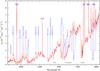 |
Fig. 1 The best part of the spectrum of V4332 Sgr obtained with Subaru/HDS in June 2009 (red). The spectrum has been smoothed and dereddened with EB−V = 0.32 and RV = 3.1 (see text for details). The strongest emission features are identified. Parts affected by telluric absorption bands are indicated by horizontal bars at the bottom. |
3.1. Photospheric spectrum
A photospheric spectrum, characteristic of a late type star, can be easily recognized in Fig. 1. When compared with earlier spectroscopic observations (Banerjee & Ashok 2004; Tylenda et al. 2005; Kimeswenger 2006), the present spectrum displays much more pronounced wide and deep absorption bands in the red part. This obviously suggests a later spectral type and a lower effective temperature. We constrained the spectral type of the present photospheric spectrum. The Subaru/HDS spectrum, corrected for interstellar extinction with EB−V = 0.32 (see Sect. 4), was compared to a grid of observed spectra of late type giants with luminosity classes III–II, taken from Bagnulo et al. (2003)5 and Gunn & Stryker (1983). The result is shown in Fig. 2, where the giant (luminosity class III) spectra of types M 4, M 5, M 6, and M 7 are plotted against the spectrum of V4332 Sgr. From this comparison we can classify the V4332 Sgr spectrum as M 5–6. This can be compared with spectral types K 8–M 3 derived from observational data in 2003 (Tylenda et al. 2005; Kimeswenger 2006). The decline in the spectral type most probably took place in 2006–2007 when the object was gradually fading in BVR, as noted in Sect. 1. The derived spectral type of the 2009 spectrum corresponds to an effective temperature of Teff ≃ 3300 K (Richichi et al. 1999). We have also fitted standard photometric spectra of luminosity class III to the BVRcIcJ photometric data presented in Sect. 7. (We used the same procedure as in Tylenda et al. 2005) The best fit gives a spectral type of M 6.2 and Teff ≃ 3200 K.
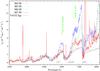 |
Fig. 2 The 2009 spectrum of V4332 Sgr (red – the same as in Fig. 1) compared to spectra of M-type giants taken from Bagnulo et al. (2003)5 and Gunn & Stryker (1983). The regions suspected of being affected by some “extra” molecular absorption are indicated by vertical green marks. |
We were not able to constrain the luminosity class of the object, except that it is a giant. There are no clear signs of absorption features of CaH, characteristic of spectra of late-type dwarfs.
The observed spectrum of V4332 Sgr differs from any standard spectrum of a late-type giant. In addition to the obvious presence of emission features, we noticed extra absorption bands not observed (or being much weaker) in stars of spectral types close to M 6 III. Most striking is the B–X absorption band of VO in the range ~7334–7534 Å, which is more characteristic of giants earlier than M 6. Some extra absorption can also be found in the range ~6985–7050 Å; it can be assigned to the satellite branch of TiO γ (0, 0) (cf. Kamiński et al. 2009), but this identification is very tentative. The regions contaminated by the extra absorption features are indicated in Fig. 2.
A possible explanation for the difference between the observed spectrum of V4332 Sgr and the standard spectra of giants could be the peculiarities in the object’s metallicity. We compared the Subaru/HDS spectrum with a grid of MARCS spectra (Gustafsson et al. 2008) with Teff = 3200 K, log g = 0.0, M = 1 M⊙, standard chemical composition, and metallicity in the range −2 ≤ [ Fe/H ] ≤ + 0.5 (see the table on http://marcs.astro.uu.se). The shape of the observed spectrum is best represented by the model spectrum with [Fe/H] = −1.5. The fit is still not perfect but no extra absorption is needed in the 7500 Å region; however, Martini et al. (1999) obtained fits to the spectra observed during the 1994 outburst using models with solar abundances. Our suggestion of a low metallicity in V4332 Sgr is very tentative. The object is not a typical giant, so peculiarities in the spectrum are expected. Besides, as discussed in Sect. 7, we probably do not observe the object directly, but rather a part of its spectrum that is scattered on a disc matter. Scattering can affect the shape of the spectrum.
Measurements for the resonance emission lines seen in the Subaru spectrum of V4332 Sgr.
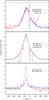 |
Fig. 3 Profiles of the strong resonance lines in the spectrum of V4332 Sgr. Spectra are rescaled. The vertical lines mark the centre of the K i lines at –69 km s-1 and the centre of interstellar absorption features of Na i at –7.2 km s-1. Top: the Na i profiles, clipped for clarity. The top spectrum shows the intensity-inverted profile of the H i 21 cm line (see text). Middle: the observed K i lines and a theoretical Lorentzian profile. The strongest telluric absorption lines are indicated. Bottom: Ca i and Rb i lines, spectra slightly smoothed to reduce the noise. |
We did not find any atomic absorption features that could be identified as photospheric lines. A photospheric absorption line of Ca i 6572 Å, relatively strong in late type giants, may be the cause of the irregular shape of the observed Ca i emission profile, as discussed in Sect. 3.2. No photospheric signatures were found within the profiles of the Na i and K i doublets.
The lack of atomic absorption lines in the photospheric spectrum does not allow us to derive a reliable value of the radial velocity of the object. As can be seen from Fig. 1, most of the photospheric absorption bands coincide with narrow components in emission. However, in a few cases relatively clean band-heads without emission component can be seen and their position measured. This is the case for the following TiO γ bands: (3, 2) R1 (6849 ± 1.0 Å), (4,3) R1 (6917.6 ± 0.5 Å), (5, 4) R1 (6987.4 ± 1.0 Å), (0, 0) SR21 (7036.7 ± 0.5 Å), and (3, 4) R3 (7818.6 ± 0.5 Å). These measurements give rough estimates of the (heliocentric) radial velocity of the object, i.e., −40, −56, −45, −67, and −60 km s-1, respectively. These values imply a heliocentric radial velocity of the source of the photospheric spectrum of −56 ± 16 km s-1.
3.2. Atomic emission lines
The strongest atomic emission lines seen in the Subaru/HDS spectrum are listed in Table 1. They are characterized in terms of observed wavelength, heliocentric radial velocity (Vh), full width at half-maximum (FWHM), integrated flux, and equivalent width (EW). For the K i and Na i doublets, we also present “cleaned” fluxes, which are fluxes measured for the lines after removing all atmospheric and interstellar absorption features from their profiles. The fluxes are not corrected for interstellar reddening. We do not present any measurements of EW for the Na i doublet since the observed continuum in the region of these lines is very faint. Some of the strongest emission lines are indicated in the spectrogram presented in Fig. 1. Their profiles are displayed in more detail in Fig. 3.
The profiles of the emission lines are triangular in shape and their cores can be reproduced well by a Lorentzian profile (see Fig. 3, middle panel); however, the observed wings are significantly less extended than in the Lorentzian profile. The emission lines appear to be fairly symmetric. Only with the mirror profile-inverting procedure or by over-plotting a theoretical profile on the observed ones can some asymmetry be noticed (see Fig. 3). The Ca i line shows a clear sign of asymmetry, with a stronger blueshifted half of the profile, but this may be an effect of a non-flatness of the underlying continuum or a contamination by a photospheric absorption line (if present).
3.3. Molecular bands in emission
All the identified molecular emission features are listed in Table 2. Columns 1, 2 of the table contain the observed and laboratory wavelengths of the feature. Columns 3, 4 show the name of the molecule and identification of the electronic system, vibrational band, and the branch forming the head. Column 5 presents the heliocentric radial velocities of those features for which a unique assignment was reliable. Column 6 shows the integrated fluxes of the emission lines (for which reliable measurements were possible), while Col. 7 lists their equivalent widths. Comments on the nature of the features are given in Col. 8, while the sources of the laboratory wavelengths can be found in Col. 9.
The laboratory wavelengths refer to the band-head positions. When a sharp band-head is recognized in the spectrum, the observed wavelength corresponds to the position of the band-head. These values have been used when determining the radial velocities. In the other cases, the observed wavelengths are the positions of apparent maxima of the emissions. In the case of the VO B4Π–X bands, the four emission features correspond to the four sub-bands formed by the main branches concentrated around the sub-band origin.
The emission fluxes were measured by integrating the surface above the continuum. The continuum position has usually been determined by an inspection of the VLT/UVES spectra of the M 5 III, M 6 III, and M 7 III stars (HD 214952, HD 189124, and HD 18242, respectively) (Bagnulo et al. 2003). In rare cases of gaps in the comparison spectra, a theoretical spectrum was synthesized to exclude the possibility of strong underlying absorptions. Large errors in the flux measurements of the VO B4Π–X (0, 0) are mainly due to uncertainties in the underlying continuum.
A detailed analysis of the profiles of the bands is presented in Sect. 5
3.4. Interstellar features
The only features that can be ascribed to the interstellar medium (ISM) are the Na i 5889/5895 and K i 7664/7698 doublets in absorption. No diffuse interstellar bands were found in the spectrum. We determined radial velocities, FWHMs, and EWs of the interstellar features by fitting Gaussian profiles. Before performing a fitting procedure, the appropriate regions of the spectrum were normalized with high order polynomials to correct for the broad emission features that form a steep baseline for the interstellar features. The results of Gaussian fits are listed in Table 3. The errors of the EWs reflect only a statistical error, which was determined from a series of independent measurements for each line. The FWHMs given in Table 3 are not corrected for the instrumental broadening. The FWHM of the instrumental profile, as measured from the narrowest telluric lines seen in the spectrum, is on average 8.0 km s-1, so the profiles of the interstellar features are mostly resolved.
As can be seen in Table 3, there is a shift of about 4 km s-1 between the peaks of the Na i and K i lines. The shift may be physical, but it can also be partially caused by the fact that the Na i absorption lines are saturated or close to saturation.
The interslellar absorption features seen in the spectrum of V4332 Sgr can be compared to a profile of the H i 21 cm emission line in the direction of the star. From the 21 cm LAB Survey (Kalberla et al. 2005), we extracted a spectrum for a position nearest to the position of V4332 Sgr, i.e. at
 ,
,  (V4332 Sgr:
  ,
,  ). The half-power beam-width of the LAB Survey is 36′, so the position of V4332 Sgr is located close to the centre of the beam for the extracted position. The profile of the H i line is composed of several narrow components, tightly blending into one complex profile. The intensity-inverted and rescaled spectrum of H i is shown in Fig. 3 (top panel). A Gaussian fit to the overall profile gives a central velocity of Vh = −6 km s-1. The profiles of the absorption lines of K i and Na i lie well within the profile of H i. The interstellar absorption lines seen in the optical spectrum indicate that the line of sight towards V4332 Sgr crosses most, if not all, of the ISM in this direction. This conclusion agrees with an analysis of extinction of V4332 Sgr in Kimeswenger (2007).
4. Reddening, distance, radial velocity
Analyses of spectroscopic and photometric observations of V4332 Sgr during its outburst in 1994 have led Martini et al. (1999), Tylenda et al. (2005), and Kimeswenger (2006) to conclude that the reddenning to the object is EB−V = 0.32 ± 0.02, EB−V = 0.32 ± 0.10, and EB−V = 0.37 ± 0.07, respectively.
The reddenning can be estimated from a relation between EWs of atomic interstellar absorption lines and EB−V. Using the relation derived in Munari & Zwitter (1997), our measurement for the K i 7699 line from Table 3 results in EB−V = 0.45 ± 0.05. We did not use the Na i D lines since they reach zero flux in our spectrum and are probably saturated.
Molecular emissions.
We also used the Galactic Dust Extinction Service6, which estimates EB−V from the 100 μm dust emission mapped by IRAS and COBE/DIRBE. This tool is based on a method that gives good constraints on the extinction for regions with low-to-moderate reddening. For the position of V4332 Sgr, we get EB−V = 0.344 ± 0.008.
An independent constraint on the reddening can be obtained from the radio observations of the H i 21 cm line. The integrated intensity of the H i line of 664.2 K km s-1 can be converted to a column density of N(Hi) = 1.25 × 1021 cm-2 using a standard conversion factor of 1.822 × 1018 cm-2 (K km s-1)-1 (e.g., Wilson et al. 2009). The value of the reddening can be found from a relation given by Bohlin et al. (1978). By neglecting a contribution from molecular hydrogen (our observations in the CO rotational transition, see Sect. 2.3, show no molecular cloud in the direction of V4332 Sgr) we get EB−V = 0.22 ± 0.04. In the present paper we adopt EB−V = 0.32 as a reasonable compromise between the above estimates.
The distance to V4332 Sgr is unknown. Martini et al. (1999) estimated that the object is at ~300 pc. Assuming that the progenitor of V4332 Sgr was a main sequence star, Tylenda et al. (2005) estimated a distance of ~1.8 kpc. A lower limit to the distance can be obtained from the observed radial velocities of the interstellar absorption lines. A mean heliocentric radial velocity derived from the values listed in Table 3 is −5.5 km s-1. This corresponds to VLSR = 6.5 km s-1. After adopting a Galactic rotation curve of Brand & Blitz (1993), we find that V4332 Sgr is at a distance ≳ 1.0 kpc. This excludes the low distance value of Martini et al. (1999).
As noted in Tylenda et al. (2005), the radial velocity of V4332 Sgr shows that the object does not follow the Galactic rotation. The present analyses of the photospheric spectrum, atomic emission lines, and molecular bands give Vh = −56 ± 16 km s-1 (Sect. 3.1), −65 ± 7 km s-1 (Table 1), and −75 ± 10 km s-1 (Table 2), respectively. These values are less negative than those estimated in Martini et al. (1999) (−180 km s-1) and Tylenda et al. (2005) (−160 km s-1), but are still noticeably different from what is expected from the Galactic rotation in the direction of V4332 Sgr (≳ −12 km s-1, heliocentric). Thus there is no way to estimate the kinematic distance of the object.
Results of Gaussian fits to the ISM absorption features found in the Subaru/HDS spectrum of V4332 Sgr from June 2009.
In the present paper, we adopt, if required, a distance of 1.8 kpc (following Tylenda et al. 2005). This is a very uncertain value, but the principal conclusions drawn in the present paper are independent of the distance.
5. Analysis of the molecular bands in emission
The main question that arises when analysing the observed molecular bands in emission concerns mechanism(s) that could produce these features. One should be able to consider collisional excitation and/or radiative pumping of excited states of the molecules as a primary source of the emissions. As is shown below, the observed band profiles can only be reproduced if the rotational temperature is assumed to be very low, typically ~120 K. This implies that the kinetic temperature must also be close to it in the ambient medium. In these conditions there is no way to significantly populate the observed upper electronic states by collisions, because they would require temperatures of a few thousand K, meaning that the only possibility that remains is the radiative pumping. Molecules at ground states absorb radiation photons capable of exciting them to higher electronic levels. Radiative decays from them produce the observed emissions. The analysis done in this section assumes this mechanism.
For each molecule considered in the following subsections, we have constructed a molecular model including rotational levels of the ground and excited electronic states. Molecular data for the TiO bands were taken from Schwenke (1998). The source references for VO and ScO are the same as in Kamiński et al. (2009). Generally, our models of the molecular structure included rotational levels up to the quantum number J = 65.
The population of the rotational levels of the ground state, including spin substates, is assumed to follow the Boltzman law at a given rotational temperature. The upper electronic state (together with its rotational levels) is assumed to be populated by radiative transitions from the ground state. The source of exciting radiation has usually been approximated by a blackbody of 3200 K (expected effective temperature of an M 5–6 III star). In the case of the TiO bands, a synthetic spectrum from a model stellar atmosphere of Teff = 3200 K and log g = 0.0 has been calculated (see Kamiński et al. 2009, for details). Atmospheric models of Hauschild et al. (1999) were used for this purpose. Level populations under the above conditions were solved with the code RADEX (van der Tak et al. 2007). Assuming radiative decays of the excited electronic state, a synthetic emission can be calulated from the derived populations. Due to the noise of the observed spectrum, both the observed and calculated spectra have been smoothed out (typically with an FWHM of 2.4 Å) before comparing them.
5.1. TiO
Numerous bands of titanium oxide are observed in our spectrum. Usually narrow emission components at the positions of the molecular band-heads are superimposed on broad and deep absorption bands of the photospheric spectrum. The most prominent examples are three emission components of the TiO γ (0, 0) band at 7052, 7086, and 7129 Å. We made a model analysis of these three emission components of the TiO γ (0, 0) band. The results are presented in Fig. 4.
As can be seen from the figure, the emission components overlay a broad absorption photospheric component of the same band with a relatively sharp blue edge at the position of the F3–F3 emission component at ~7050 Å. Therefore, for the purpose of the present analysis of the emission profile, we subtracted a synthetic stellar spectrum, calculated with Teff = 3200 K and log g = 0.0, from the observed one (upper part of Fig. 4). The result is shown in the lower part of Fig. 4.
The very first conclusion from the model analysis is that reliable fits to the individual emission components can be obtained only if the rotational temperature is assumed to be 120 ± 20 K. For an increasing temperature, the red tail of each component becomes more pronounced and more extended toward longer wavelengths.
Another conclusion can be drawn from the observed flux ratio, which is 2:1:3 for the F3–F3, F2–F2, and F1–F1 components, respectively. Since the upper substates of each component are connected with the lower substates only by main branches (satellite ones are very weak), it can be assumed that all the three emission components are uncoupled transitions. Then, differences in the fluxes can be caused by different populations of the lower substates and/or by differences in the flux pumping the upper levels. Assuming that the lower levels are populated according to the Boltzman distribution with a temperature of 120 K, we find that the ratio of the F1–F1 and F2–F2 fluxes is consistent with the optically thin limit. Effectively, the lowest rotational levels of the F3 substate (with energies from 400 to 520 cm-1) are about 2 times less populated than the lowest rotational levels of the F2 substate, and 4 times less than those of the lowest F1 substate. If the pumping flux is similar for the three transitions, the expected value of the above flux ratio is therefore 1:2:4. The observed F3–F3 component is thus significantly enhanced. An assumption of optically thick emissions would only flatter this ratio. The enhanced emission of the F3–F3 component could be explained if the flux illuminating the emitting area in this transition were significantly higher than the fluxes pumping the remaining two. As can be seen from Fig. 4 (upper part) the F3–F3 component (at ~7050 Å) is situated on the strong blue edge of the photospheric absorption band. Thus, if the emitting region escapes from the source of the photospheric radiation, the edge of the photospheric band is redshifted and a significant enhancement of the pumping radiation is then available for the F3–F3 component compared to the F1–F1 and F2–F2 components. Our modelling shows that the observed flux ratio can be satisfactorily reproduced if the photospheric spectrum, as seen by the emitting region, is redshifted by at least 25 km s-1. The resulting emission profiles, calculated for a relative velocity between the photospheric source and the emitting gas of 40 km s-1, are shown in the lower part of Fig. 4.
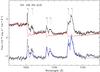 |
Fig. 4 Upper part: the observed spectrum in the vicinity of the TiO γ (0, 0) band (black line) and a synthetic model spectrum for Teff = 3200 K and log g = 0.0 (red line). Lower part: result of subtraction of the synthetic stellar flux from the observed one (black line) and the model emission calculated as explained in the text (blue line). |
5.2. ScO and YO
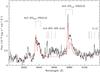 |
Fig. 5 The observed spectrum around the ScO A2Σ–X |
In the observed spectrum, both ScO A2Π–X (0, 0) and YO A2Π–X (0, 0) bands are present in emission. The rotational contours of ScO sub-bands, A
 –X and A
 –X, are shown in Fig. 5. A grid of theoretical profiles have been synthesized for a range of rotational temperatures. The best fit to the observed spectra is obtained for a rotational temperature of 120 ± 20 K and a radial velocity of −75 ± 10 km s-1 (Fig. 5).
Emission of yttrium oxide A–X (0, 0) at 6133 Å is rather weak and barely recognizable. The second component A–X (0, 0) of YO is not seen in the spectrum.
5.3. VO
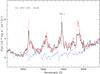 |
Fig. 6 The observed spectrum near the emission band of VO B3Π–X |

Vanadium oxide B4Π–X (in short B–X) (0, 0) and (1, 0) bands are seen as prominent emission features (see Fig. 1 and Table 2). The most intense B–X (0, 0) band is shown in detail in Fig. 6. The band consists of four sub-bands formed by the main branches. A model fit to the data suggests a rotational temperature of ~100 K, in agreement with the rotational temperature derived above for the TiO bands.
The observed spectrum around the VO B–X (0, 0) band has a relatively high S/N. Comparing this part of the spectrum with the UVES spectrum of HD 18242 (M 7 III), we can estimate the radial velocity of the photospheric spectrum. From the sharp absorption feature (probably due to VO in the photosphere) at 7960.4 Å, as well as the nearby TiO band head at 7818.6 Å, we estimate the heliocentric stellar velocity to be −60 ± 20 km s-1.
A final fit was obtained by summing the predicted rotational countour of the VO B–X band and the spectrum of HD 18242. The best fit (shown in red in Fig. 6) was obtained for a velocity of emitting gas of −75 ± 5 km s-1. The observed spectrum also shows the VO C–X (1, 0) and (0, 0) bands around 5474 Å and 5736 Å, respectively. They appear as narrow emission features, which are too weak and too noisy to be analysed in more detail.
5.4. CrO
After having identified the atomic and molecular emission features in the observed spectrum, we are left with a few broad (~20 Å) emission-like features in the spectral range between 5800 and 6800 Å. We postulate that they come from the electronic band system B5Π–X5Π of CrO observed in emission, as shown in Fig. 1. Details of the proposed identification can be found in Table 2.
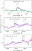 |
Fig. 7 Detailed view of CrO B5Π–X5Π bands in emission. The observed spectra are plotted with a black line, while theoretical contours of the CrO bands are shown as a blue line. An M 7 III spectrum is displayed in magenta in the middle and bottom panels. A synthetic spectrum is shown in green in the top panel. |
We have identified five vibronic bands of CrO, i.e. (1, 0), (0, 0), (0, 1), (0, 2), and (2, 3), shown in Figs. 7 and 5. The expected positions of the (1, 2) and (1, 1) bands are also marked in the figures. The broad emission profiles are due to overlapping of five sub-bands formed by main branches.
Relative intensities of the emission bands with a common upper vibrational state can be compared with theoretical predictions. For this purpose we used Franck-Condon factors computed by Reddy et al. (1998). We find that the predicted ratios are fairly consistent with the observed fluxes. The ratios of the emission fluxes of the (1, 0):(1, 1):(1:2) bands are predicted to be 3.0:0.1:2.0, while the observed ones are 7:0: ≲ 1, respectively. The observed ratios of the (0, 0):(0, 1):(0:2) bands are 3.5:4.8:3.4 compared with the theoretical predictions of 3:4:2, respectively.
We synthesized the expected contours of the CrO emission features. A line list from the laboratory work of Hocking et al. (1980) was used. Rotational intensities were computed consistently from diagonalization of Hamiltonians defined by Hocking et al. (1980) and using the standard approach (see e.g. Hougen 2001). The computed strenghts were checked to reproduce analytical formulas of rotational intensities of Kovacs (1969). The molecular structure included in the model is rather complex and consists of the four lowest vibrational levels of the ground state and the three lowest vibrational levels of the upper electronic state. Each vibrational level is composed of five substates and each substate is composed of lower rotational levels up to J = 65, in order to include levels with energies up to 2400 cm-1. All the radiative transitions between the listed levels are included.
To reproduce the observed shapes of the rotational contours, a rotational temperature of the ground state of 450 K was assumed. This relatively high rotational temperature (compared to that derived from the above analysis of other molecules) is needed to explain formation of all the five band heads seen in the observed spectrum, as well as their trapezoidal shapes. The exciting radiation was simulated by a blackbody of 3200 K. The obtained theoretical contours are shown in Fig. 7. They have been shifted by –70 km s-1 to fit the observed features.
Because of the reasonable consistency between the observed and predicted wavelength positions, rotational contours (as expected from environment of low kinetic temperature), intensity ratios, and the presence of all the expected bands, we consider the identification of the CrO B–X system in the spectrum of V4332 Sgr as reliable. CrO was said to be seen in the atmosphere of β Pegasi (spectral class M 2) by Davies (1947) on the basis of band-head mesurements. Later, on this finding was questioned by Jorgensen (1996). Our identification is the first detection of CrO in emission in any astrophysical environment.
6. Origin of the emission features
Two important conclusions have been drawn from our model analysis of the observed molecular bands in emission in Sect. 5. First, these features are produced by radiative pumping. Second, the emitting gas is escaping from the source of the pumping radiation (Sect. 5.1).
If the molecular emission bands are formed by radiative pumping then it is natural to suppose that the atomic emission lines are also produced in the same mechanism. All the atomic lines observed in our spectrum in emission are from resonance transitions. In this case it is difficult, if not impossible, to avoid radiative pumping in the atomic lines, if this mechanism is effective for the molecular bands; both photoabsorption cross sections and the expected abundances are larger for elements like Na and K than for molecules like TiO, VO, or ScO.
As can be seen from Table 1, the observed ratio of the Na i D lines (5890/5896 Å) is close to 1.0. The same ratio for the K i lines (7665/7699 Å) is ~1.2. In an optically thin case both ratios are expected to be 2.0. The fact that the line ratio in the Na i and K i doublets is observed to be close to 1.0, can be very easily and naturally explained within the hypothesis of radiative pumping. The line intensity in this mechanism is limited by the flux of the pumping spectrum. Since the number of photons available for each line of a given doublet is practically the same in the pumping spectrum (assumed to be stellar-like), already for a moderate thickness (of a few) in the lines, the line ratio must approach 1.0.
In terms of intensities, the K i doublet dominates the spectrum in the observed spectral range. It is ~25 times stronger that the Na i doublet. The high K i/Na i flux ratio is rather unusual. In most circumstellar environments, when both doublets are observed, the Na i lines are stronger thanks to the ~16 times higher abundance. (The transition probabilities for both doublets are very close). The relative K i and Na i line strengths observed in V4332 Sgr can be easily explained, if they are assumed to be pumped by radiation. As discussed above, the observed line ratios indicate that the lines absorb almost all the available pumping radiation. Therefore the observed K i/Na i flux ratio is expected to reflect the spectral energy distribution of the underlying photospheric source. The flux ratio of the observed photospheric continuum near the K i and Na i doublets can be estimated from the photometry in the IC and V bands, respectively (effective wavelengths of these photometric bands are close to the wavelengths of the doublets). By adopting IC = 15.1 and V = 19.7 (see Sect. 7) and using the standard Vega flux calibration, one gets λFλ(7680Å)/λFλ(5890 Å) ≃ 28. Another way to estimate the above ratio is to measure the continuum from our Subaru spectrum. Near the Na i doublet, the observed contiunnum is very faint but it can be estimated as Fλ(5890Å) ≃ 1 × 10-17 erg s-1 cm-2 Å-1. In the vicinity of the K i doublet, we measure Fλ(7680 Å) ≃ 1.7 × 10⁻¹⁶ erg s-1 cm-2 Å-1. This results in λFλ(7680 Å)/λFλ(5890 Å) ≃ 22. Both estimates are in excellent agreement with the observed flux ratio of the K i and Na i doublets, confirming our hypothesis that the emission lines observed in the spectrum of V4332 Sgr are indeed pumped by the photospheric radiation of the central source.
As can be seen from Table 1, the EWs of the Ca i and Rb i lines are almost two orders of magnitude lower that those of the K i lines. This implies that the former lines are optically thin; i.e., they absorb only a small part of the available photospheric photons. This statement is confirmed by the expected low abundance of Rb and the low transition probability in the Ca i (intercombination) line. The difference in the optical thickness is probably also the reason for the observed differences in the profiles, namely that the Ca i and Rb i lines are significantly narrower compared to those of K i and Na i (see column 6 in Table 1).
We have shown that the spectral shape of the observed photospheric spectrum of M 5-6 III can explain both the shape of the TiO γ (0, 0) band (Sect. 5.1) and the flux ratio of the K i/Na i doublets. However, in the observed spectrum we do not see any absorption features, which could be interpreted as from photons absorbed in the pumping mechanism. This shows that we do not see any absorbing matter along the line of sight and implies that the matter seen in the emission features is not distributed spherically around the continuum source. The observed continuum is also much too faint to be able to pump emission features as strong as observed. As can be seen from Fig. 1, peak intensities in some molecular features and particulary in the atomic lines are by large factors higher than the intensity of the underlying continuum. The observed EWs of the K i lines (see Table 1) imply that if they had been excited by the observed continuum in their vicinity, they would have had to absorb all the continuum photons from a spectral region as large as ~550 Å. This would be possible only if the absorbing matter had been moving with a velocity gradient, between slowest and fastest regions, as large as ~20 000 km s-1, which is two orders of magnitude higher than the velocities observed in V4332 Sgr during its eruption (Martini et al. 1999). Therefore we conclude that the photospheric continuum responsible for pumping the observed emission features is much stronger than the observed one. The above discussion of the K i lines suggests that we observe ≲1% of the flux emitted by the central object. In Sect. 7 we further argue that the central object in V4332 Sgr is mostly hidden to us by an opaque disc seen almost edge-on.
7. Spectral energy distribution
The SED of V4332 Sgr was already investigated by Tylenda et al. (2005). It was based on photometric data obtained in 2003 and covering photometric bands from B to M. Tylenda et al. (2005) point out that apart from the stellar-like component dominating in the optical and near-IR, the object displayed a large IR-excess seen in the KLM bands. When interpreted as a single blackbody the IR component had an effective temperature of ~750 K and a luminosity ~15 times higher than that of the optical component. Another possibility mentioned in Tylenda et al. (2005) was an accretion disc ~25 times more luminous than the central star.
Figure 8 displays an SED of V4332 Sgr derived from various observations obtained between April 2005 and May 2009. The source of the data are as follows:
-
Optical photometric measurements were taken from the webpage of V. Goranskij7.These are combined data from different observatories. Weinterpolated the BVRCIC magnitutes for the date of the Subaru/HDS observations and adopted B = 21.4, V = 19.7, RC = 17.9, IC = 15.1 mag. The error bars shown in Fig. 8 for the optical magnitudes represent a scatter in the photometric measurements around the date of the Subaru/HDS observations.
-
The JHKS data are from the observations reported on in Sect. 2.2.
-
IR measurements in the LMNn bands were taken from Lynch et al. (2006), and they correspond to observations carried out on 7 August 2006.
-
Far-IR data were taken from Banerjee et al. (2007). These are Spitzer/MIPS fluxes at 24 μm, 70 μm, and 160 μm averaged from measurements obtained on 15 October 2005 and 2 November 2006.
-
AKARI measurmements were taken form the first releases of the FIS Bright Source Catalogue (Yamamura et al. 2010) and IRC Point Source Catalogue (Kataza et al. 2010), which are based on observations from the AKARI All-Sky Survey performed in 2006–2007. For the AKARI Infrared Camera (IRC), the source was detected only in the 9 μm band with flux density of 507.7 mJy. Reliable measurements with the Far-Infrared Surveyor instrument (FIS) are available only for the 65 μm and 90 μm bands with density fluxes of F65 = 1.79 Jy and F90 = 1.13 Jy. There are also data for the FIS bands at 140 and 160 μm (F140 = 86.9 mJy and F160 = 29.9 mJy), but the measurements are flagged as unreliable (too weak a source at those bands). The total (absolute and relative) calibration uncertainty of the measurements in all the AKARI bands is 20% (3σ; Yamamura et al. 2010; Kataza et al. 2010).
-
In Fig. 8 we also display spectra of V4332 Sgr in wide spectral ranges. The optical spectra are the Subaru/HDS spectrum reported in this paper and a synthetic spectrum from the MARCS grid (Gustafsson et al. 2008) with Teff = 3200 K, solar metalicity, and log g = 0.0; the last was rescaled to fit the fluxes of the Subaru/HDS data. The Spitzer spectra are also shown. They were acquired on 18 April 2005 and 27 September 2005.
Vega fluxes were used as zero points when converting magnitudes to flux-density units. The optical spectra and the BVRCICJHKS data points shown in Fig. 8 are corrected for interstellar reddening with EB−V = 0.32 and RV = 3.1.
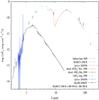 |
Fig. 8 Spectral energy distribution for V4332 Sgr. Observational points are taken from different sources as listed in the text. Our attempt to fit the observed SED is shown with a dashed line. |
In the following discussion we assume that the object did not vary significantly between 2005 and 2009. This is not entirely justfied since, as noted in Sect. 1, the object faded in the optical in 2006; however, it seems that the overall SED has remained more or less unchanged over a few recent years. When compared with the photometric data in 2003 (Tylenda et al. 2005), the object is now ~1.5 mag fainter in BVR but ~1.0 mag brighter in JHK. Banerjee et al. (2007) note that the object remained constant over a year in their far-IR observations in 2005–2006.
Similar to Tylenda et al. (2005), the SED in Fig. 8 displays a huge IR-excess. However, thanks to the far-IR data, we can now conclude that it cannot be represented by a single temperature component. We have attempted to reproduce it in Fig. 8 with a sum of two blackbodies of 950 K and 200 K, but it would be more reasonable to conclude that this is a multi-temperature component with temperatures ranging between these two values. This result, combined with the fact that the IR component has remained stable since at least 2003, strongly suggests that we see a multi-temperature Keplerian disc of matter surrounding the central object resembling an M 5–6 giant.
In the simple fit to the observed points in Fig. 8 the two IR components, i.e. blackbodies of 950 K and 200 K, are ~30 and ~20 times more luminous, respectively, than the stellar component of Teff = 3200 K. Assuming spherical geometry of the components, the two infrared components would have radii ~65 and ~1200 times larger than the stellar one. If interpreted with a disc-like spectrum, the disc would have an apparent luminosity ~50 times higher than the central star.
In principle, one can consider two possible sources of energy radiated away by a disc, i.e., reproduction of the central star radiation absorbed by the disc matter (so-called passive disc) or gravitational energy dissipation by viscous forces transferring matter from outer disc layers to inner ones and eventually to the star surface (accretion disc). In both cases, the central star is expected to be at least as bright as the disc. In the first case (passive disc), for obvious geometrical reasons the disc can absorb, hence reradiate, only a part of the stellar luminosity. In the second case (accretion disc), the accreted matter is expected to release a comparable energy to what is dissipated in the disc, at the star surface (so-called disc boundary layer), where the matter has to slow down from the Keplerian velocity to the velocity of stellar rotation (usually much lower than Keplerian). In the case of a giant or a supergiant, the boundary-layer braking is likely to take place below the photosphere. In this case, accretion is expected to add a luminosity to the intrinsic stellar luminosity, similar to that of the disc.
The only way to reconcile that the central star in V4332 Sgr is observed to be ~50 times less luminous that the disc is to assume that the disc is observed almost edge-on. In this case the disc would block most of the stellar radiation in the direction to the observer. The geometrical aspect (inclination close to 90°) means that the observed lumnosity of the disc is also expected to be significantly lower than the true one. Therefore we can conclude that the stellar component observed in the optical only accounts for ≲1% of the luminosity of the central object in V4332 Sgr. This conclusion nicely fits the one drawn from our analysis of the emission features in Sect. 6.
8. Discussion
Our analysis done in Sects. 6 and 7 has led us to conclude that V4332 Sgr is now observed as consisting of a central object, resembling an M 5–6 giant, surrounded by a disc of circumstellar matter. The inclination angle of the disc is close to 90°, so that the disc matter obscures the central star, and we can only observe a tiny part of its radiation. The situation thus resembles what is observed in IRAS 18059–3211, known as Gomez’s Hamburger (Ruiz et al. 1987; Wood et al. 2008), whose global SED is similar to V4332 Sgr. The central star in Gomez’s Hamburger is not directly seen, and the observed optical spectrum is entirely due to scattering of the central star radiation on dust grains in the outer edge of the disc. It is very probable that the same situation is also observed in V4332 Sgr. Polarimetric observations in the optical would allow verification of this hypothesis.
Molecular bands in emission have been observed in the optical spectrum of the luminous red supergiant VY CMa (Herbig 1974; Wallerstein & Gonzalez 2001, and references therein), as well as of U Equ (Barnbaum et al. 1996). In both cases it has been suggested that the objects are surrounded by massive circumstellar discs, which obscure the central stars along the line of sight (Herbig 1970; Kastner & Weintraub 1998; Barnbaum et al. 1996), i.e. similar to what we propose in the present paper for V4332 Sgr. The existence of a disc obscuring the central star thus seems to be a condition favouring observations of molecular bands in emission. Indeed, if we increased the photospheric spectrum in V4332 Sgr by a factor of 100 (as suggested in Sects. 6 and 7, if the central star were unobscured) remaining the fluxes of the emission features unchanged, then we would have practically no chance to detect any emission molecular band. The only visible emission features would then be those of K i and Na i.
As shown in Sect. 3.1, the spectral type of the observed photospheric spectrum agrees with the BVRcIc photometry corrected for the interstellar extinction. Thus the scattering responsible for the observed photospheric spectrum has no significant effect on its global shape. This can be understood if the observed spectrum is mainly produced by forward scattering on the outer disc rim lying in front of the central star, as we suggest for V4332 Sgr. In this case scattering is dominated by large grains (a ≳ 0.3 μm), which have a high value of g ≡ ⟨ cosθ ⟩ , i.e. scatter mainly in forward directions. These grains also have Qsca that is practically independent of wavelength in the optical (e.g. Loar & Draine 1993)8.
As discussed in Sect. 6, the emission features observed in V4332 Sgr are most likely pumped by radiation from the central star. One may ask where the matter seen in the emission features can be situated. One possibility is that this could be matter in the atmosphere of the disc. However, the profiles of the emission lines observed in V4332 Sgr are single-peaked (see Fig. 3), while it is widely believed that emission features observed from an edge-on disc should be double-peaked (due to the disc rotation). Although this is true in most cases, there are situations where disc emission lines can be observed as single-peaked. Simulations of Murray & Chiang (1996, 1997) show that this happens when the disc is seen at a high inclination angle and possesses a wind, which is optically thick in the lines. This mechanism could explain the profiles of the Na i and K i lines, since, as discussed in Sect. 6, these lines are most likely optically thick. However, as discussed in the same section, the Ca i and Rb i lines are optically thin, and yet they are single-peaked (see Fig. 3). Another problem arises from the observed line wings extending up to ~ ± 250 km s-1 from the line centre (see Fig. 3). If formed in a high-inclination disc, they would measure the rotation velocity of the innermost observable regions of the disc. Adopting a distance of V4332 Sgr of ~1.8 kpc (following Tylenda et al. 2005, who obtained this value after assuming that the progenitor was a solar type star), our fit to the optical photometry (mentioned in Sect. 3.1) results in an effective radius of ~5 R⊙ (similarly to the one derived in Tylenda et al. 2005, for 2003). However, as we now know, the true central star is probably two orders of magnitude brighter than observed and thus has a radius that is an order of magnitude larger than the above estimate. For a solar-mass star and a radius of ~50 R⊙ one obtains a Keplerian velocity of ~60 km s-1 at the stellar surface. Since the central star is obscured and thus the disc regions up to a few stellar radii are also unseen, there seems to be no way to explain the line wings extending up to ~ ± 250 km s-1 within the idea of the emission lines arising from the disc. A higher stellar mass would make the situation even worse. For instance, a 3 M⊙ progenitor would be almost two orders of magnitude brighter and about 10 times more distant, and the outburst remnant would be 10 times more extended, lowering the Keplerian velocity at its surface by a factor of 2.
It thus seems that we are only left with a scenario, in which the emission features are formed in matter lost by the central object. This idea is in accord with our findings in Sect. 5.1 that the observed ratio of the emission components of the TiO γ (0, 0) band implies an outflow velocity of the emitting matter of at least 25 km s-1. The origin of the outflowing matter could be matter ejected in the past, e.g. during the 1994 outburst, or a wind flowing out at present from the object, or both. The low rotational temperature found from the molecular bands in emission (Sect. 5) suggests that these features are formed in a cold medium, thus at significant distances from the central object. This seems to favour the former possibility of matter ejected in the past. The observed widths of the atomic lines at zero intensity (see Fig. 3) imply an outflow velocity of up to ~250 km s-1. The line profiles suggest that the outflow is concentrated along an axis nearly perpendicular to the line of sight. This could be the axis of the disc. Detailed modelling of the line profiles would be required to better constrain the structure and nature of the outflow.
See the web page of Gornaskij: http://jet.sao.ru/~goray/v4332sgr.htm
Acknowledgments
We would like to thank the group of support astronomers at the Carlos Sánchez Telescope, especially R. Barrena, for obtaining the service photometric observations reported in this paper. This research made use of the NASA/ IPAC Infrared Science Archive, which is operated by the Jet Propulsion Laboratory, California Institute of Technology, under contract with the National Aeronautics and Space Administration. We acknowledge the use of data from the UVES Paranal Observatory Project (ESO DDT Programme ID 266.D-5655). This research is also partly based on observations with AKARI, a JAXA project with the participation of ESA. The research reported on in this paper has partly been supported by a grant no. N203 004 32/0448 financed by the Polish Ministery of Sciences and Higher Education.
References
- Bagnulo, S., Jehin, E., Ledoux, C., et al. 2003, The Messenger, 114, 10 [NASA ADS] [Google Scholar]
- Banerjee, D. P. K., & Ashok, N. M. 2004, ApJ, 604, 57 [Google Scholar]
- Banerjee, D. P. K., Varricatt, W. P., Ashok, N. M., & Launila, O. 2003, ApJ, 598, L31 [NASA ADS] [CrossRef] [Google Scholar]
- Banerjee, D. P. K., Varricatt, W. P., & Ashok, N. M. 2004, ApJ, 615, 53 [Google Scholar]
- Banerjee, D. P. K., Misselt, K. A., Su, K. Y. L., Ashok, N. M., & Smith, P. S. 2007, ApJ, 666, L25 [NASA ADS] [CrossRef] [Google Scholar]
- Barnbaum, C., Omont, A., & Morris, M. 1996, A&A, 310, 259 [NASA ADS] [Google Scholar]
- Bohlin, R. C., Savage, B. D., & Drake, J. F. 1978, ApJ, 224, 132 [NASA ADS] [CrossRef] [Google Scholar]
- Brand, J., & Blitz, L. 1993, A&A, 275, 67 [NASA ADS] [Google Scholar]
- Buckle, J. V., Hills, R. E., Smith, H., et al. 2009, MNRAS, 399, 1026 [NASA ADS] [CrossRef] [Google Scholar]
- Davis, D. N. 1947, ApJ, 106, 28 [NASA ADS] [CrossRef] [Google Scholar]
- Gunn, J. E., & Stryker, L. L. 1983, ApJS, 52, 121 [NASA ADS] [CrossRef] [Google Scholar]
- Gustafsson, B., Edvardsson, B., Eriksson, K., et al. 2008, A&A, 486, 951 [NASA ADS] [CrossRef] [EDP Sciences] [Google Scholar]
- Hamuy, M., Walker, A. R., Suntzeff, N. B., et al. 1992, PASP, 104, 533 [NASA ADS] [CrossRef] [Google Scholar]
- Hamuy, M., Suntzeff, N. B., Heathcote, S. R., et al. 1994, PASP, 106, 566 [NASA ADS] [CrossRef] [Google Scholar]
- Hauschildt, P. H., Allard, F., Ferguson, J., Baron, E., & Alexander, D. R. 1999, ApJ, 525, 871 [NASA ADS] [CrossRef] [Google Scholar]
- Herbig, G. H. 1970, ApJ, 162, 557 [NASA ADS] [CrossRef] [Google Scholar]
- Herbig, G. H. 1974, ApJ, 188, 533 [NASA ADS] [CrossRef] [Google Scholar]
- Hocking, W. H., Merer, A. J., Milton, D. J., Jones, W. E., & Krishnamurty, G. 1980, Can. J. Phys., 58, 516 [NASA ADS] [Google Scholar]
- Hougen, J. T. 2001, The Calculation of Rotational Energy Levels and Rotational Line Intensities in Diatomic Molecules (version 1.0), available at: http://physics.nist.gov/DiatomicCalculations [2009, December 9], National Institute of Standards and Technology, Gaithersburg, MD [Google Scholar]
- Jorgensen, U. G. 1996, in Molecules in Astrophysics: Probes & Processes, ed. E. van Dishoeck, IAU Symp., 178, 441 [Google Scholar]
- Kalberla, P. M. W., Burton, W. B., Hartmann, D., et al. 2005, A&A, 440, 775 [NASA ADS] [CrossRef] [EDP Sciences] [Google Scholar]
- Kamiński, T., Schmidt, M., Tylenda, R., Konacki, M., & Gromadzki, M. 2009, ApJS, 182, 33 [NASA ADS] [CrossRef] [Google Scholar]
- Kastner, J. H., & Weintraub, D. A. 1998, AJ, 115, 1592 [NASA ADS] [CrossRef] [Google Scholar]
- Katza, H. et al. 2010, AKARI/IRC All-Sky Survey Point Source Catalogue Version 1.0 available at http://www.ir.isas.jaxa.jp/AKARI/Observation/PSC/Public [Google Scholar]
- Kimeswenger, S. 2006, Astron. Nachr., 327, 44 [NASA ADS] [CrossRef] [Google Scholar]
- Kimeswenger, S. 2007, ASP Conf. Ser., 363, 197 [Google Scholar]
- Kovacs, I. 1969, Rotational Structure in the Spectra of Diatomic Molecules (Budapest) [Google Scholar]
- Loar, A., & Draine, B. T. 1993, ApJ, 402, 441 [NASA ADS] [CrossRef] [Google Scholar]
- Lynch, D. K., Russell, R. W., Ford, R., Hammel, H. B., & Sitko, M. L. 2006, IAU Circ., 8739, 1 [NASA ADS] [Google Scholar]
- Martini, P., Wagner, R. M., Tomaney, A., et al. 1999, AJ, 118, 1034 [NASA ADS] [CrossRef] [Google Scholar]
- Munari, U., & Zwitter, T. 1997, A&A, 318, 269 [NASA ADS] [Google Scholar]
- Murray, N., & Chiang, J. 1996, Nature, 382, 789 [NASA ADS] [CrossRef] [Google Scholar]
- Murray, N., & Chiang, J. 1997, ApJ, 474, 91 [NASA ADS] [CrossRef] [Google Scholar]
- Noguchi, K., Aoki, W., Kawanomoto, S., et al. 2002, PASJ, 54, 855 [NASA ADS] [CrossRef] [Google Scholar]
- Phillips, J. G. 1973, ApJS, 26, 313 [NASA ADS] [CrossRef] [Google Scholar]
- Reddy, R. R., Ahammed Nazeer, Y., Rama Gopal, K., Abdul Azeem, P., & Anjaneyulu, S. 1998, Ap&SS, 262, 223 [NASA ADS] [CrossRef] [Google Scholar]
- Richichi, A., Fabbroni, L., Ragland, S., & Scholz, M. 1999, A&A, 344, 511 [NASA ADS] [Google Scholar]
- Ruiz, M. T., Blanco, V., Maza, J., et al. 1987, ApJ, 316, L21 [NASA ADS] [CrossRef] [Google Scholar]
- Rosen, B. 1970, Spectroscopic Data relative to Diatomic Molecules, (Pergamon Press) [Google Scholar]
- Schöier, F. L., van der Tak, F. F. S., van Dishoeck, E. F., & Black, J. H. 2005, A&A, 432, 369 [NASA ADS] [CrossRef] [EDP Sciences] [Google Scholar]
- Schwenke, D. W. 1998, Chemistry and Physics of Molecules and Grains in Space, Faraday Discussions, 109, 321 [Google Scholar]
- Soker, N., & Tylenda, R. 2003, ApJ, 582, L105 [NASA ADS] [CrossRef] [Google Scholar]
- Tylenda, R., & Soker, N. 2006, A&A, 451, 223 [NASA ADS] [CrossRef] [EDP Sciences] [Google Scholar]
- Tylenda, R., Crause, L. A., Górny, S. K., & Schmidt, M. R. 2005, A&A, 439, 651 [NASA ADS] [CrossRef] [EDP Sciences] [Google Scholar]
- van der Tak, F. F. S., Black, J. H., Schöier, F. L., Jansen, D. J., & van Dishoeck, E. F. 2007, A&A, 468, 627 [NASA ADS] [CrossRef] [EDP Sciences] [Google Scholar]
- Wallerstein, G., & Gonzalez, G. 2001, PASP, 113, 954 [NASA ADS] [CrossRef] [Google Scholar]
- Willmarth, D., & Barnes, J. 1994, A User’s Guide to Reducing Echelle Spectra With IRAF (Tucson: NOAO) http://iraf.net/irafdocs/ech/ [Google Scholar]
- Wilson, T. L., Rohlfs, K., & Hüttemeister, S. 2009, Tools of Radio Astronomy (Berlin: Springer) [Google Scholar]
- Wood, K., Whithney, B. A., Robitaille, T., & Draine, B. T. 2008, ApJ, 688, 1118 [NASA ADS] [CrossRef] [Google Scholar]
- Yamamura, I. et al. 2010, AKARI/FIS All-Sky Survey Bright Source Catalogue Version 1.0, available at http://www.ir.isas.jaxa.jp/AKARI/Observation/PSC/Public [Google Scholar]
All Tables
Measurements for the resonance emission lines seen in the Subaru spectrum of V4332 Sgr.
Results of Gaussian fits to the ISM absorption features found in the Subaru/HDS spectrum of V4332 Sgr from June 2009.
All Figures
|
Fig. 1 The best part of the spectrum of V4332 Sgr obtained with Subaru/HDS in June 2009 (red). The spectrum has been smoothed and dereddened with EB−V = 0.32 and RV = 3.1 (see text for details). The strongest emission features are identified. Parts affected by telluric absorption bands are indicated by horizontal bars at the bottom. |
| In the text | |
|
Fig. 2 The 2009 spectrum of V4332 Sgr (red – the same as in Fig. 1) compared to spectra of M-type giants taken from Bagnulo et al. (2003)5 and Gunn & Stryker (1983). The regions suspected of being affected by some “extra” molecular absorption are indicated by vertical green marks. |
| In the text | |
|
Fig. 3 Profiles of the strong resonance lines in the spectrum of V4332 Sgr. Spectra are rescaled. The vertical lines mark the centre of the K i lines at –69 km s-1 and the centre of interstellar absorption features of Na i at –7.2 km s-1. Top: the Na i profiles, clipped for clarity. The top spectrum shows the intensity-inverted profile of the H i 21 cm line (see text). Middle: the observed K i lines and a theoretical Lorentzian profile. The strongest telluric absorption lines are indicated. Bottom: Ca i and Rb i lines, spectra slightly smoothed to reduce the noise. |
| In the text | |
|
Fig. 4 Upper part: the observed spectrum in the vicinity of the TiO γ (0, 0) band (black line) and a synthetic model spectrum for Teff = 3200 K and log g = 0.0 (red line). Lower part: result of subtraction of the synthetic stellar flux from the observed one (black line) and the model emission calculated as explained in the text (blue line). |
| In the text | |
|
Fig. 5 The observed spectrum around the ScO A2Σ–X |
| In the text | |
|
Fig. 6 The observed spectrum near the emission band of VO B3Π–X |
| In the text | |
|
Fig. 7 Detailed view of CrO B5Π–X5Π bands in emission. The observed spectra are plotted with a black line, while theoretical contours of the CrO bands are shown as a blue line. An M 7 III spectrum is displayed in magenta in the middle and bottom panels. A synthetic spectrum is shown in green in the top panel. |
| In the text | |
|
Fig. 8 Spectral energy distribution for V4332 Sgr. Observational points are taken from different sources as listed in the text. Our attempt to fit the observed SED is shown with a dashed line. |
| In the text | |
Current usage metrics show cumulative count of Article Views (full-text article views including HTML views, PDF and ePub downloads, according to the available data) and Abstracts Views on Vision4Press platform.
Data correspond to usage on the plateform after 2015. The current usage metrics is available 48-96 hours after online publication and is updated daily on week days.
Initial download of the metrics may take a while.