| Issue |
A&A
Volume 522, November 2010
|
|
|---|---|---|
| Article Number | A71 | |
| Number of page(s) | 23 | |
| Section | Galactic structure, stellar clusters and populations | |
| DOI | https://doi.org/10.1051/0004-6361/201014392 | |
| Published online | 04 November 2010 | |
Search for extratidal features around 17 globular clusters in the Sloan Digital Sky Survey
1
Astronomisches Rechen-Institut, Zentrum für Astronomie der Universität
Heidelberg,
Mönchhofstrasse 12-14,
69120
Heidelberg,
Germany
e-mail: jordi@ari.uni-heidelberg.de
2
Department of Physics, University of Basel,
Klingelbergstrasse 82,
4056
Basel,
Switzerland
Received:
9
March
2010
Accepted:
2
August
2010
Context. The dynamical evolution of a single globular cluster and also of the entire Galactic globular cluster system has been studied theoretically in detail. In particular, simulations show how the “lost” stars are distributed in tidal tails emerging from the clusters.
Aims. We investigate the distribution of Galactic globular cluster stars on the sky to identify such features as tidal tails. The Sloan Digital Sky Survey provides consistent photometry of a large part of the sky to study the projected two-dimensional structure of the 17 globular clusters in its survey area.
Methods. We used a color–magnitude weighted counting algorithm to map (potential) cluster member stars on the sky.
Results. We recover the already known tidal tails of Pal 5 and NGC 5466. For NGC 4147 we find a two-arm morphology. Possible indications of tidal tails are also seen around NGC 5053 and NGC 7078, confirming earlier suggestions. Moreover, we find potential tails around NGC 5904 and Pal 14. Especially for Palomar clusters other than Pal 5, deeper data are needed to confirm or to rule out the existence of tails. For many of the remaining clusters in our sample we observe a pronounced extratidal halo, which is particularly large for NGC 7006 and Pal 1. In some cases, the extratidal halos may be associated with the stream of the Sagittarius dwarf spheroidal galaxy (e.g., NGC 4147, NGC 5024, NGC 5053).
Key words: globular clusters: general / Galaxy: structure
© ESO, 2010
1. Introduction
Globular clusters (GCs) are the oldest stellar objects found in the Milky Way (MW), with ages in the range of 10–13 Gyr. They represent tracers of the early formation history of our Galaxy. GCs are ideal systems for studying stellar dynamics in high-density systems because their relaxation times are much shorter than their age (Gnedin & Ostriker 1997, GO97). At least in the cluster core, we expect the stars to have lost memory of their initial conditions. The GCs we see today are only the lucky survivors of an initially much larger population (GO97). Several different mechanisms can dissolve a GC: internal processes include infant mortality (Geyer & Burkert 2001; Kroupa 2001) by stellar evolution, gas expulsion, and two-body relaxation. External mechanisms primarily include the interaction of the GC with the constantly changing tidal field of its host galaxy.
Different processes are dominant at different ages of the cluster. For young clusters, stellar evolution is the main driver that may potentially cause them to dissolve. More massive stars are evolving rapidly. They have strong winds and explode as supernovae within the first few million years driving out the remaining gas. The sudden change due to the mass loss in the GC’s internal gravitational field can destroy the GC. Two-body relaxation arises from close encounters between cluster stars, leading to a slow diffusion of stars over the tidal boundary. This process takes place from the beginning to the final dissolution of the cluster. Equipartition of energy by two-body encounters leads to mass segregation. The more massive stars sink to the center, while less massive stars remain in the outer parts of the cluster. This usually leads them to lose low-mass stars, which can be observed today in declining mass-function slopes of GCs (Baumgardt & Makino 2003). On the other hand, the mass loss from the cluster’s encounter with the Galactic disk and bulge is strongest at pericenter passages, especially for GCs on elliptical orbits (Baumgardt & Makino 2003). All these mechanisms have one common result: the GC is losing stars. As a result of relaxation, stars gradually diffuse out, while the GC’s loss of stars is more sudden during tidal shocks.
Among the observational studies, Grillmair et al. (1995) performed deep two-color star counts to examine the outer structure of 12 GCs using photographic Schmidt plates. They detected a halo of extratidal stars around most of their clusters. They also found indications of possible tidal tails emerging from some clusters. The tidal tails are not purely of stellar origin in all cases, as the morphological identification of galaxies and stars, especially for faint objects, was not perfect; i.e., in some cases, background galaxies were mistaken for stars. In other cases random overdensities of foreground stars induced features into the cluster’s contours. Leon et al. (2000) studied the tidal tails of 20 GCs, using Schmidt plates as well. These authors also find halos of extratidal stars, as well as tidal features for most of their clusters. The two studies have three GCs in common. For two out of the three clusters, Grillmair et al. (1995) detected tidal tails where Leon et al. (2000) did not see such a strong signal, and in the third case it is the opposite.
Globular clusters in the SDSS DR7 footprint.
Among the theoretical studies, Gnedin & Ostriker (1997) (GO97) studied the dynamical evolution of the entire Galactic GC system. They derived the destruction rates due to the internal and external mechanisms. According to their calculations, the total destruction rate of the entire GC system is such that more than half of the present day GCs will not survive the next Hubble time. GO97 did not include any information on the GCs’ proper motion, they used the known present day distance to the Galactic center and the GCs’ radial velocity.
Dinescu et al. (1999, DG99) derived the destruction rates for a smaller sample of Galactic GCs in a similar way, but included the measured proper motion data. They concluded that the destruction processes for the clusters in their sample are mostly dominated by internal relaxation and stellar evaporation. Tidal shocks due to the bulge and disk are only dominant for a small number of GCs in their sample. For the sample we are studying here this is only the case for Pal 5. Comparing their destruction rates with the numbers of GO97, they find that the GO97 total rates are larger. The destruction rates due to internal processes (2-body relaxation, stellar evaporation) are comparable in both studies, therefore only the destruction rate due to tidal shocks is incompatible. DG99 conclude that the statistical approach of assigning tangential velocities (the method used by GO97) results in more destructive orbits than are actually observed.
A similar conclusion is drawn by Allen et al. (2006), who derived the orbits of Galactic GCs, also based on observed proper motions, in an axisymmetrical potential and in a barred potential (resembling the MW). They derived the destruction rates for the GCs in their sample in an almost identical way to DG99. Allen et al. (2006) further investigated the influence of the bar on the clusters’ orbits and destruction rates. The bar does not influence the orbits of clusters that have a pericenter distance greater than ~4 kpc. Hence, none of the clusters in our sample (see Table 1) are influenced by the bar.
Combes et al. (1999) studied the tidal effects experienced by GCs on their orbits around the MW. In general, they find that two long tidal tails should emerge extending out to 5 tidal radii. They conclude by stating i) GCs are always surrounded by tidal tails and tidal debris; ii) the tails are preferentially composed of low mass stars; iii) mass loss in a GC is enhanced if the cluster is rotating in the direct sense with respect to its orbit; iv) extended tidal tails trace the cluster’s orbit; and v) stars are not distributed homogeneously along the tidal tails, but clump.
Capuzzo Dolcetta et al. (2005) investigated the clumpy structure of the tidal tails. They found that the clumpy structure is not associated with an episodic mass loss or tidal shocks due to encounters with Galactic substructure, as stars are continuously lost. The clumps are not self-gravitating systems. Küpper et al. (2008) showed that the clumps are a result of epicyclic motion of the stars lost by the cluster. Just et al. (2009) investigated the formation of the clumps and discussed their observability. Küpper et al. (2010) investigate the position of the clumps relative to the cluster for clusters on eccentric orbits. They concluded that tidal shocks are not the direct origin of the clumps. Further, Capuzzo Dolcetta et al. (2005) confirmed the earlier finding that the cluster’s leading tail develops inside the orbit, while the trailing tail follows outside the orbital path. They also found that for clusters on elliptical orbits the tidal tails trace the orbital path only near perigalacticon (see also Dehnen et al. 2004). On the other hand for circular orbits the tails are clear tracers of the cluster path. Moreover the length of the tails is not constantly growing. On eccentric orbits the leading tail tends to be longer than the trailing tail during the cluster’s motion from apogalacticon to perigalacticon and vice versa during the other half of the cluster’s orbit.
Montuori et al. (2007) investigated the direction of tidal tails with respect to the GC’s orbit. In the outer parts of the tails (> 7–8 tidal radii away from the cluster center), the tails are very well aligned with the cluster’s orbit regardless of the cluster’s location on the orbit. On the other hand, in the inner parts, the orientation of the tidal tails is strongly correlated with the orbital eccentricity and the GC’s location on the orbit. Only if the cluster is near perigalacticon, the inner tidal tails are aligned with the orbital path. Therefore, only if long tidal tails are detected, it is possible to securely constrain the cluster’s orbit from those. Detecting only small, short tidal extensions just outside the GC’s tidal radius do not give any hint on the cluster’s orbit unless the cluster’s proper motion has been measured before.
DG99 published proper motions of a large number of GCs and added values from the literature to their catalog. From this they derived orbital parameters, such as ellipticity e, perigalacticon Rperi, apogalacticon Rapo, etc. The eleven clusters we have in common with DG99 have orbital eccentricities higher than ~0.3, i.e., there are no circular orbits for our sample.
These studies give a good theoretical understanding of the size, shape, orientation, etc. of tidal tails of GCs.In an observational study of light element abundance variations in field halo stars, Martell & Grebel (2010) conclude that as many as half of the stars in the Galactic halo may originally have formed in meanwhile dissolved GCs. In this paper we use data from the Sloan Digital Sky Survey to study the 2D structure of 17 Milky Way GCs and to compare the observed features with the theoretical predictions. The paper is organized as follows: Sect. 2 introduces the photometric data used in our analysis. Section 3 explains the algorithm used to count (potential) member stars on the sky. In Sect. 4 we present the number density profiles of the 17 clusters in our sample. Section 5 presents the derived contour maps for our GCs. In Sect. 6 we discuss our results. The paper is concluded in Sect. 7 with a summary.
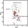 |
Fig. 1 Vital diagram from GO97. The red stars are the GCs in our sample. Cluster mass and half-light radius were taken from GO97. GCs within the triangles are most likely surviving the next Hubble time. Adopted from G097, reproduced by permission of the AAS. |
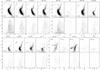 |
Fig. 2 Top rows: color–magnitude diagrams of all GCs in our sample in order of increasing distance from the Sun. The distances from Harris (1996) are printed in each CMD. The gray horizontal line marks the magnitude limit for each cluster. Bottom rows: color–magnitude diagrams of a random field in the vicinity of the cluster (see text for details). |
2. Data
The Sloan Digital Sky Survey (SDSS) is an imaging and spectroscopic survey in the Northern hemisphere (York et al. 2000). SDSS imaging data are produced in the five bands ugriz (Fukugita et al. 1996; Gunn et al. 1998; Hogg et al. 2001; Smith et al. 2002; Ivezić et al. 2004; Tucker et al. 2006; Gunn et al. 2006). The data are automatically processed to measure photometric and astrometric properties (Lupton et al. 2002; Pier et al. 2003, Photo) and are publicly available on the SDSS web pages1. We used the data from the SDSS Data Release 7 (DR7, Abazajian et al. 2009).
The automatic SDSS pipeline Photo was initially designed to process high Galactic latitude fields with a low density of Galactic field stars. Fields centered on and around GCs are too crowded for Photo to process, so the automatic pipeline does not provide photometry for these most crowded regions. An et al. (2008, An08) used the DAOPHOT crowded-field photometry package to derive accurate photometry for the stars in these crowded areas. This photometry is published on the SDSS web pages as a value-added catalog2. From this catalog we only considered stars with photometry flags set to 0. The An08 catalog and the original SDSS catalog overlap around each GC. If a star is measured in both samples, we used the original SDSS photometry. This choice has no influence on the result. Finally, we merged the two datasets into one catalog for each GCs. The magnitudes in the final catalog were corrected for extinction. The SDSS catalog provides the Galactic foreground extinction values from Schlegel et al. (1998). For the fields with An08 photometry, the extinction values were derived by a cubic interpolation of the values listed in the SDSS catalog.
In Table 1 we list the GCs found in the SDSS DR7 footprint. Columns (3) and (4) contain the equatorial coordinates (J2000.0) of the cluster center mainly taken from Harris (1996), except for Pal 14 (Hilker 2006) and NGC 7089 (Dalessandro et al. 2009). In Col. (5) we list the clusters’ distance to the Sun and in Col. (6) the clusters’ distance to the center of the MW from Harris (1996), except for Pal 14 (Hilker 2006). Columns (7) and (8) contain the core and tidal radii from McLaughlin & van der Marel (2005, M05). For almost all GCs in our sample proper motions have been measured. Only for three of the most distant GCs, NGC 2419, Pal 4 and Pal 14, as well as for NGC 5053 this information is lacking. Columns (9) and (10) list the proper motion taken from DG99.
In Fig. 2 we show the color–magnitude diagrams (CMDs) (g-r,g) of all GCs in our sample in order of increasing distance from the Sun (see Col. 5 in Table 1). We show all stars within the clusters’ tidal radii. In the bottom panels we show for each GC a sample of field stars. The field stars are chosen from a random field in the vicinity of the GC (~2° away) within a circle equal to the clusters’ tidal circle.
The SDSS data were taken over several years and in different observing conditions. The average seeing is 1.5″ (Adelman-McCarthy et al. 2007). In our study we only use the g, r, and i bands. Ivezić et al. (2004) showed that stellar population colors are constant over the survey area, concluding that the photometric calibration is accurate to roughly 0.02 mag. Further, Ivezić et al. (2007) analyzed multiple observations of bright stars in the southern equatorial stripe. The photometry was repeatable to less than 0.01 mag in all five bands.
3. Counting algorithm
To map cluster member stars on the sky we used the same method as Odenkirchen et al. (2003) to follow the tidal tails of Pal 5. We refer the reader to Odenkirchen et al. (2003) for a detailed description of the procedure. Here, we only give a rough overview.
For the subsequent study of the distribution of stars on the sky we need a clean sample of
potential member stars. In order to reduce the contamination of our sample with field stars
we define new orthogonal color indices:  In
a color–color plot the cluster stars are located in an almost one-dimensional locus. The new
indices were now chosen in such a way that the color c1 traces
the cluster stars’ locus and c2 is perpendicular to that. To
derive these indices for each GC we used the stars within
2 / 3·rt, where
rt is the cluster’s tidal radius from Table 1. We fitted a straight line
y = tan(α)·x + b to
the distribution of stars in the color-color diagram
(g − r) vs. (g − i),
where x represents the (g − r) axis and y
the (g − i) axis. In Table 2 we list the fitted parameters tan(α) and b
from which we derived k1 = cos(α),
k2 = sin(α),
k3 = − b·sin(α), and
k4 = − b·cos(α) for each
GC.
In
a color–color plot the cluster stars are located in an almost one-dimensional locus. The new
indices were now chosen in such a way that the color c1 traces
the cluster stars’ locus and c2 is perpendicular to that. To
derive these indices for each GC we used the stars within
2 / 3·rt, where
rt is the cluster’s tidal radius from Table 1. We fitted a straight line
y = tan(α)·x + b to
the distribution of stars in the color-color diagram
(g − r) vs. (g − i),
where x represents the (g − r) axis and y
the (g − i) axis. In Table 2 we list the fitted parameters tan(α) and b
from which we derived k1 = cos(α),
k2 = sin(α),
k3 = − b·sin(α), and
k4 = − b·cos(α) for each
GC.
Parameters to derive the new color indices.
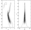 |
Fig. 3 Color magnitude diagrams (c1,g) and (c2,g). Plotted are stars of NGC 6341 within one third of the cluster’s tidal radius. The gray solid lines denote the borders within which the stars were selected. |
We selected our stars in the CMDs (c1,g) and (c2,g) to minimize the contamination by Galactic field stars. Figure 3 shows the CMDs (c1,g) and (c2,g) of NGC 6341. In (c2,g) we selected all stars with | c2 | < 2.5·σ(c2)(g). σ(c2)(g) is the rms dispersion in c2 for stars of magnitude g. Stars with deviating c2 colors are unlikely to be cluster members.
In (c1,g) we selected all stars within 3σ of the cluster’s ridge line. The ridge line of a GC traces the location of highest density of stars in a CMD. Figure 3 shows the selection criteria for NGC 6341 as an example. This preselection leaves us with the final catalog, where all stars are explicitly chosen to have the same photometric properties as the GC, but are located not only at the position of the cluster but also in the wide field around it. The final catalog is then split into the cluster sample to contain all stars within 2 / 3·rt and the field sample to contain all stars outside 3 / 2·rt. If a cluster was observed to be more extended than previously thought, we redefined the two samples. In some cases, e.g., for NGC 5024 and NGC 5053, two clusters are close neighbors in the projection on the sky. In these cases, we excluded all stars within the tidal radius of the neighboring cluster from the field sample.
The stars in the preselected samples are not simply counted. The ratio of the distribution of cluster stars to field stars in the CMD (c1,g) was used as a weight in the sum. Figure 4 shows the two Hess diagrams of NGC 5272. The left panel is the field sample, the right panel the cluster sample. The cluster sample shows a prominent main sequence and subgiant branch. Furthermore, a red giant and horizontal branch are visible. For the field sample, the density is more homogeneous in the entire selected areas. The horizontal branch is only prominent at the red edge.
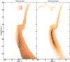 |
Fig. 4 Hess diagrams of the field (left panel) and cluster (right panel) sample of NGC 5272. Only stars already selected in c1 and c2 were used. |
The density of cluster stars nC(k) at a given
point k on the sky is thus given as 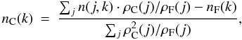 (3)where
ρC and ρF are the density
distribution of the cluster and field sample, respectively, in the CMD (see Fig. 4). nF is the average
background in the field around the GC.
(3)where
ρC and ρF are the density
distribution of the cluster and field sample, respectively, in the CMD (see Fig. 4). nF is the average
background in the field around the GC.
From Eq. (3) we see that each star in a
given cell on the sky k and in color-magnitude space j is
weighted according to its position in the CMD by the factor
ρC(j) / ρF(j).
This weighted number of stars per cell on the sky is then summed and divided by the factor
 . This gives the estimated
number of cluster stars nC plus a term
nF / a, the number of
contaminating field stars attenuated by a.
. This gives the estimated
number of cluster stars nC plus a term
nF / a, the number of
contaminating field stars attenuated by a.
4. Number density profiles
The large area coverage of the SDSS data allows us to study the number density profiles of GCs further out than any survey before. By using a large area “far away” from the cluster we are able to determine the mean background contamination and to investigate in detail the outer boundaries of the GCs.
We derived the number density profiles by counting the stars in concentric annuli of constant width dr. We used only the stars preselected in colors and magnitude as described above. We used annuli of width 2′ outside the tidal radius. Within the cluster’s tidal radius we chose either 0.5′ or 1′ as width of the annuli, depending on the surface density of the cluster. An alternative way to derive the number density profile would be by using annuli containing a constant number of stars. Comparing these two methods revealed no differences in the resulting profiles and parameters.
For the final number density profile we counted all stars in each annulus and divided by the area of the annulus. The error of the number density was derived by dividing the annulus in 20 segments. We then derived the number of stars in each segment and used the standard deviation of these 20 values as the error. For clusters with a small number of stars we divided the annuli in 8 segments to reduce the effect of small number statistics.
For the denser clusters the SDSS is not suited to observe the number density profile in the cluster’s central part due to crowding. Therefore, we combined the number density profiles from the SDSS with previously published profiles for the inner parts of the GCs. The surface brightness profiles by Trager et al. (1995, T95) and the revised study of the same data by McLaughlin & van der Marel (2005, M05) are the only large catalogs of surface brightness profiles of Galactic GCs. We combined these datasets with our new SDSS profiles to get profiles ranging from the cluster center out to several times the tidal radius. In order to combine the two datasets, we converted the surface brightness μ(r) of T95 into a number density log (N(r)) = − μ(r) / 2.5 + C. C is a constant derived separately for each GC in the following way. The T95 profile and the SDSS profile overlap within a certain radial range. This overlap was used to derive the vertical shift C between the profiles. The T95 profiles were shifted by C to match the SDSS profiles. For GCs whose T95 profiles extend far out, the outermost points were not taken into account, because these data points are the most affected by the background contamination or subtraction. Furthermore, differences in the outer parts of the different profiles can also be explained by mass segregation in the clusters, unveiled by different limiting magnitudes.
Measured structural parameters.
For the GCs NGC 5272 (M 3), NGC 5904 (M 5), NGC 6205 (M 13), NGC 6341 (M 92), NGC 7078 (M 15), and NGC 7089 (M 2) Noyola & Gebhardt (2006, N06) published surface brightness profiles derived from HST observations. They tested the influence of the chosen filter on the profiles and found no dependence. The profiles looked the same in each observed filter. For 50% of their clusters the photometric data points are brighter in the central parts of the clusters than the fitted King profiles (King 1962). The discrepancy between the observations and the fit increases as the radius decreases. N06 conclude that the inner parts are not suited to be fitted with a King profile.
For these six GCs we combined the N06 profiles and our SDSS profiles to span the widest possible range in radius. The combination was done in an identical way as for the combination of the T95 sample with our SDSS profiles.
The combined profiles were fitted with King (1962) and Plummer (1911) profiles. For the King profiles, we adopted the background levels derived from the SDSS observations and determined the core and tidal radius through our fit. For the Plummer profiles we derived the Plummer radius rp through our fit. In Figs. 5–7 we show the combined number density profiles of all clusters in our sample. Table 3 lists the fitted core and tidal radii, the observed stellar background density nbkg and the Plummer radius. For some GCs, e.g. NGC 5466, NGC 6205, the Plummer profile provides a better fit than the King profile. But in most cases, the Plummer profile does not trace the observed number density profile. Peñarrubia et al. (2009) found that a Plummer profile more accurately traces the profile of a stellar system (mainly a dwarf spheroidal galaxy) that loses mass due to tidal effects. For NGC 5466 this is certainly the case and the known tidal tails are proof of tidal mass loss. For Pal 5, which is also known for its long tidal tails, the Plummer profile is not a better fit than the King profile. In the following Section we will discuss the prominent features and trends in the density profiles for each cluster individually.
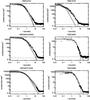 |
Fig. 5 Number density profiles of NGC 2419, NGC 4147, NGC 5024, NGC 5053, NGC 5272, and NGC 5466. The black open squares show the combined profiles. The black filled squares were derived in this study. The light gray solid line is the best fit King profile. The dark gray line is the best fit Plummer profile. The horizontal line marks the measured, mean background nbkg. |
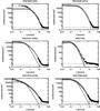 |
Fig. 6 Number density profiles of NGC 5904, NGC 6205, NGC 6341, NGC 7006, NGC 7078, and NGC 7089. The black open squares show the combined profiles. The black filled squares were derived in this study. The light gray solid line is the best fit King profile. The dark gray line is the best fit Plummer profile. The horizontal line marks the measured, mean background nbkg. |
 |
Fig. 7 Number density profiles of Pal 1, Pal 3, Pal 4, Pal 5, and Pal 14. The black open squares show the combined profiles. The black filled squares were derived in this study. The light gray solid line is the best fit King profile. The dark gray line is the best fit Plummer profile. The horizontal line marks the measured, mean background nbkg. |
In Figs. 8–24 we plot our newly derived tidal radii as red ellipses. The tidal radius, rt, from the King (1962) profiles is the radius at which the stellar density (number of stars per arcmin2) drops to zero. It must not necessarily be the radius outside of which a star has left the cluster potential, but it is an estimate of this radius. The radius outside of which the star left the cluster potential is the distance between the cluster center and the first Lagrangian point, the Jacobi radius (Baumgardt et al. 2010). Stars outside the Jacobi radius have left the GC’s potential. Baumgardt et al. (2010) calculated Jacobi radii for all Galactic GCs. We adopted these values. In Figs. 8–24 the Jacobi radii are plotted as blue dashed ellipses.
5. Tidal features
In all contour maps we plot iso-density lines at levels of
1,2,3,5,7,8,10,20,40,60,80,100,200,400,600,800,1000,
2000·σbkg above the mean weighted background level
 . The mean weighted background
was derived at least two tidal radii away from the cluster and if there were unusable areas,
e.g., close neighboring clusters, overlapping SDSS scans, areas outside the SDSS footprint,
known tidal tails, etc., these were not taken into account for its determination.
σbkg denotes the standard deviation of the weighted density in
the area, which was used to determine . The mean
weighted background, , is
different from the background nbkg derived in Sect. 4. nbkg is the mean of the
number of stars per area, whereas for
. The mean weighted background
was derived at least two tidal radii away from the cluster and if there were unusable areas,
e.g., close neighboring clusters, overlapping SDSS scans, areas outside the SDSS footprint,
known tidal tails, etc., these were not taken into account for its determination.
σbkg denotes the standard deviation of the weighted density in
the area, which was used to determine . The mean
weighted background, , is
different from the background nbkg derived in Sect. 4. nbkg is the mean of the
number of stars per area, whereas for  the stars
were weighted by the factor
ρC(j) / ρF(j)
according to their position in the CMD.
the stars
were weighted by the factor
ρC(j) / ρF(j)
according to their position in the CMD.
In Figs. 8–24 we present the contour maps for all 17 GCs in our sample. The upper/left panel shows a large area, typically 9deg by 9deg, in order to show potential large scale features in a Lambert conical projection. The lower/right panels show a blow-up in order to study the small scale tidal structures of the GCs. On the x-axis of the zoom-in plots we plot the coordinate RAshown = Xm + (RA − Xm)·cos(Ym), where (Xm, Ym) is the center of the cluster. All contour plots have North up and East left. The calculated iso-density contours are smoothed with a Gaussian kernel over 5 pixels (= 15 arcmin) with a sigma of 2 pixels (= 6 arcmin). In all maps the 1σbkg and the 2σbkg are shown in gray, while the higher contours are shown in black.
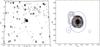 |
Fig. 8 Left panel: contour plot of a large area centered on NGC 2419. Right panel: blow-up of the contour plot centered on NGC 2419. In both panels the isodensity lines are drawn at levels of 1,2,3,5,7,8,10,20,40,····σbkg above the mean weighted background level. The 1σbkg and 2σbkg contours are drawn in light gray, the higher levels are drawn in black. The solid gray arrow points towards the Galactic Center. The gray solid line marks the edge of the SDSS survey area. The red solid circle shows the King tidal radius. The blue dashed circle shows the Jacobi radius. |
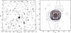 |
Fig. 9 Same as Fig. 8 but for NGC 4147. The gray dashed arrow indicates the direction of its Galactic motion based on the proper motions stated in Table 1. |
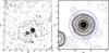 |
Fig. 10 Same as Fig. 8 but for NGC 5024. The high overdensity in the left panel at (199, 17.8) is the GC NGC 5053. The solid black line denotes the area observed by Chun et al. (2010). |
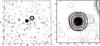 |
Fig. 11 Same as Fig. 8 but for NGC 5053. The high overdensity in the left panel at (198, 18) is the GC NGC 5024. |
Before presenting all contour maps, we briefly discuss the possible sources for contamination.
-
Background galaxies & quasars. The SDSS automatic Star/Galaxy separation seems to be very reliable. As we only use data considered to be a point source we, in principle, do not have to worry about contaminating background galaxies or galaxy clusters. In the fields with An08 photometry this may be an issue, but these fields do have a high stellar density, with stars outnumbering contaminating galaxies. As quasars are point sources and are included in the SDSS database together with stars, these might influence our data. We have looked at the SDSS quasar catalog IV (Schneider et al. 2007), which contains 77429 quasars from SDSS DR5. We applied the same selection criteria in color and magnitude to select possible contaminating quasars for each GCs, respectively. E.g., for NGC 5272 we end up with 54 quasars contaminating our sample of 51964 stars in total. The contamination due to quasars can be neglected.
-
Dust. Extinction by dust might also influence our tidal features. All our magnitudes are corrected for extinction as given in the SDSS database by values from Schlegel et al. (1998) . In a first look, we do not expect a strong contamination by dust, as the SDSS mainly observed the sky around the North Galactic pole (NGP), where less dust is expected. But, in previous studies a correlation between tidal tails and dust was found for some GCs. We examined for each GC the orientation of the tidal features and studied the potential correlation with the dust. We did not observe any correlation.
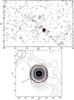
Fig. 14 Same as Fig. 8 but for Pal 5. The overdensity at (229.5, 2) in the upper panel is the GC NGC 5904.
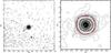
Fig. 15 Same as Figure 8 but for NGC 5904. The overdensity at (229,0) in the left panel is the GC Pal 5.
-
Foreground and background stars. In Sect. 3 we explained our criteria to select stars in color-magnitude space to minimize the number of stellar foreground and background contaminants. For all GCs we have only selected stars within 3σ of the cluster’s ridge line to assure that the majority of stars counted are likely cluster members. The 2D distribution of these selected stars shows in all cases a unique maximum at the GC’s position. The area around the GC is in all cases not perfectly flat, but shows density peaks of various significances. I.e., we are able to clean our stellar sample, but not perfectly. A more accurate exclusion of Galactic foreground and background contaminants can only be achieved with spectroscopic confirmations for each single star – a task which seems almost impossible for the time being.
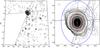 |
Fig. 17 Same as Fig. 8 but for NGC 6341. The solid gray lines denote the edge of the SDSS footprint. The dashed gray line marks the area where the stellar density was doubled (see text for details). |
5.1. NGC 2419
NGC 2419 is a very bright, unusually large GC located at a very large distance from the center of the Milky Way (RMW = 91.5 kpc, H96). Previous studies of its surface brightness profile revealed some evidence for extratidal stars (Bellazzini 2007) and references therein). In Fig. 5 our combined number density profile is shown. We also observe a break in the profile’s slope. No proper motion information is available. As NGC 2419 is very remote, only the upper part of the red-giant branch and the horizontal branch are visible in the SDSS data.
A stripe north of NGC 2419 has an artificially doubled background density. We corrected for this. All stars in the area denoted by the dashed gray line were studied. If two stars were closer than 2″ and similar in color and magnitude one of the stars was deleted from the sample. In Fig. 8 we show the resulting contour map. The average background level is 1.21 × 10⁻¹ stars arcmin-2. We detect overdensities several σ above the mean background. These features show sharp edges and a flat central plateau. The GC has a pronounced extratidal halo, but is mostly contained within its Jacobi radius. In the northeast we observed distorted contours. Comparable features might be visible on the cluster’s southwestern side, but on larger scales no features connected to NGC 2419 are observed. Casetti-Dinescu et al. (2009) speculated that NGC 2419 might be the nucleus of a (former) dwarf galaxy with the Virgo Stellar Stream being its tidal tail.
5.2. NGC 4147
From the position in the vital diagram (in Fig. 1)
we expect to observe some hint for the cluster’s dissolution due to relaxation. NGC 4147
is currently about 18.7 kpc from the Galactic center, close to apogalacticon
Rapo = 25.5 kpc (D99). In Fig. 9 we plot the contour map of the cluster with a weighted background level of
 stars arcmin-2.
The large area plot reveals a variable background. Overdensities of several
σ above are
detected. The close-up reveals a complex multiple arm morphology. The 1σ
contour appears to indicate S-shaped tidal arms extending over several tidal radii in
southern and northern directions. We detect a halo of extratidal stars and for the three
lowest contours we observe multiple tidal arms. Such a multiple arm morphology is
predicted by Montuori et al. (2007) for clusters on
elliptical orbits (e4147 = 0.73) close to apogalacticon.
NGC 288 (Leon et al. 2000) and Willman I (Willman et al. 2006) have a similarly complex
morphology, showing three tidal arms. Martínez Delgado
et al. (2004) investigated the CMD of NGC 4147 and of a comparison field close
by. They detected some hints for extratidal members stars. In the upper right plot of
Fig. 5 we plotted the number density profile of
NGC 4147. A break in the profile’s slope is observed.
stars arcmin-2.
The large area plot reveals a variable background. Overdensities of several
σ above are
detected. The close-up reveals a complex multiple arm morphology. The 1σ
contour appears to indicate S-shaped tidal arms extending over several tidal radii in
southern and northern directions. We detect a halo of extratidal stars and for the three
lowest contours we observe multiple tidal arms. Such a multiple arm morphology is
predicted by Montuori et al. (2007) for clusters on
elliptical orbits (e4147 = 0.73) close to apogalacticon.
NGC 288 (Leon et al. 2000) and Willman I (Willman et al. 2006) have a similarly complex
morphology, showing three tidal arms. Martínez Delgado
et al. (2004) investigated the CMD of NGC 4147 and of a comparison field close
by. They detected some hints for extratidal members stars. In the upper right plot of
Fig. 5 we plotted the number density profile of
NGC 4147. A break in the profile’s slope is observed.
Bellazzini et al. (2003a) found stars of the Sagittarius tidal arm in the vicinity of NGC 4147. They conclude that this cluster might be connected to the Sagittarius dwarf (Sgr dwarf). Recently, Law & Majewski (2010) investigated the association of MW GCs with the Sgr dwarf based on the authors’ newest Sgr model. The authors conclude, in contrast to earlier studies (e.g., Bellazzini et al. 2003a; Forbes & Bridges 2010), that NGC 4147’s association with the Sgr dwarf is of relative low confidence. It is thus unclear whether the extended features we observe are a feature of the Sgr dwarf field population. In any case, these stars are located at a similar distance as the cluster.
5.3. NGC 5024 (M 53)
NGC 5024 is, in projection on the sky, a very close neighbor of NGC 5053, although the two clusters are more than 1 kpc away from each other in radial direction. NGC 5024 is currently located about 18.4 kpc from the Galactic center close to its perigalacticon Rperi = 15.7 kpc (D99). In the middle left plot of Fig. 5 its number density profile is shown. The King model fitted to the combined profile reveals extratidal stars, a mild break in the slope is visible. In Fig. 10 we plot the contour map of the cluster. In the left panel, the contour map of the entire observed area is shown. The cluster is clearly detected as the highest density peak. In the surrounding field mostly features up to 3σ above the mean of 0.6 stars arcmin-2 are observed. Southeast of NGC 5024 the close neighbor NGC 5053 is detected, but no connection between the two is observed in contrast to the findings of Chun et al. (2010). The black solid polygon shows the area observed by Chun et al. (2010). We find a strong (9σ) overdensity at (198.2,16.3). In Fig. 11 this overdensity is not recognizable anymore. Therefore, we argue that it is an overdensity at the distance of NGC 5024. We found exactly one possible BHB/RR Lyrae star centered on the overdensity. It is still debated in the literature whether NGC 5024 is associated with the Sgr tidal stream (see Bellazzini et al. 2003b; Law & Majewski 2010). Our data do not permit us to conclude whether the overdensity is related to NGC 5024 or the Sgr stream. We found no obvious large scale structure connected with NGC 5024. The zoom-in on NGC 5024 shows interesting features. The contours are spherical and smooth not only in the cluster center, but also in the pronounced extratidal halo. The 1σ contour is strongly influenced by the background. Chun et al. (2010) also observed NGC 5024 and NGC 5053. They detected a tidal-bridge like feature around the two GCs and tidal features that may be due to dynamical interaction between the two clusters. Their findings are in contrast to our observations.
5.4. NGC 5053
NGC 5053 located about 16.9 kpc from the Galactic center. Lauchner et al. (2006) studied the 2D distribution of NGC 5053 and detected extratidal features east and west of the cluster. NGC 5053 is believed to be a member of the Sgr dSph (Bellazzini et al. 2003b). In Fig. 11 we show its contour map. In the large area contour map we see no pronounced large scale structure, but we definitely detect the GC and also random background noise up to 3σ above the mean of 4.1 × 10⁻² stars arcmin-2. The high overdensity northeast of the cluster is NGC 5024. The right panel of Fig. 11 is a zoom-in on NGC 5053. It reveals distorted contour lines. We observe a halo of extratidal stars. Towards the northeast and west the contours show a strong asymmetry. Similar features were observed by Lauchner et al. (2006). We see a one-armed tail-like extension toward the north-west. Such a structure is also seen to emerge from NGC 5024 (both in Figs. 10 and 11). Our data do not permit us to tell whether these curious one-armed features are tidal tails. Law & Majewski (2010) classify NGC 5053 as moderately likely associated with the Sgr dwarf. Therefore, it is possible that we are looking at substructure in the Sgr dwarf field population. Forbes & Bridges (2010) discuss the possibility that NGC 5053 or NGC 5024 might be the remnant nucleus of a dwarf galaxy. The number density profile is shown in the middle, right panel of Fig. 5. It is interesting to note that the density profile (Fig. 5) does not reveal a pronounced extratidal feature. Also Lehmann & Scholz (1997), on photographic plates, did not find any indications for tidal tails. Chun et al. (2010) observed NGC 5053 together with NGC 5024, and as stated earlier we do not reproduce their findings.
5.5. NGC 5272 (M 3)
NGC 5272 is 11.5 kpc away from the Galactic center, located close to apogalacticon Rapo = 13.7 kpc. Compared to other clusters in our sample NGC 5272 has a low expected destruction rate (GO97). The lower left panel of Fig. 5 shows its number density profile. The combined profile is not well fit with a King profile. The profile shows no change in slope as a hint for an extratidal halo. In Fig. 12 we show the contour map of this cluster. Generally, the contours are smooth. On the other hand the outer contours up to 3σ show distortions. The extreme distortions of the lowest contour are likely to be induced by the background. There is no large scale tidal structure observed. The background shows random density peaks of up to 3σ above the mean of 4.45 × 10⁻² stars arcmin-2. Leon et al. (2000) studied the 2D distribution of NGC 5272 and found extratidal features correlated with dust emission. Our contours do not show any correlation with the dust. Also Grillmair & Johnson (2006) investigated the 2D structure of NGC 5272 with SDSS data and did not detect any tidal structure.
5.6. NGC 5466
Belokurov et al. (2006) studied the 2D distribution of NGC 5466 with SDSS data and detected a 4°-long tidal tail. Earlier studies by Odenkirchen & Grebel (2004) and Lehmann & Scholz (1997), on photographic plates, already found indications for the tidal tails of this cluster. Grillmair & Johnson (2006) extended this tidal tail to 45°. Also, Chun et al. (2010) observed the tidal tails of NGC 5466. We also detect the long extratidal feature of NGC 5466 (Fig. 13). The northwest to southeast extension of the tidal tail is clearly visible. The contour plot of the larger area also reveals the tidal tails close to the cluster. The long extensions are hard to distinguish. There are random foreground peaks of up to 5σ above the mean of 4.5 × 10⁻² stars arcmin-2. This is also the case in the plots of Grillmair & Johnson (2006). Our detections resemble the detections of Chun et al. (2010). NGC 5466 is currently at a distance of 15.8 kpc from the Galactic center, close to its perigalacticon Rperi = 6.6 kpc (D99). The inner tidal tails are aligned with the cluster orbit as predicted by Montuori et al. (2007). Fellhauer et al. (2007) modeled the destruction of NGC 5466 and were able to reproduce the detected tidal tails. They further state that this cluster is mainly destroyed by tidal stripping at each perigalacticon, and that the destruction due to 2-body relaxation plays a minor role. This is in agreement with the destruction rates calculated by GO97.
5.7. Palomar 5
Pal 5 is located 18.6 kpc from the Galactic center. Odenkirchen et al. (2003) studied the distribution of cluster stars with SDSS data and found tidal tails spanning 10° on the sky. Already Odenkirchen et al. (2001) and Rockosi et al. (2002) found Pal 5’s tidal tails with SDSS data. Grillmair & Dionatos (2006) extended these tails to ~20°. Odenkirchen et al. (2002) measured the line-of-sight velocity dispersion of Pal 5 and concluded that the dispersion and the surface density profile are consistent with a King profile of W0 = 2.9 and rt = 16.1′, similar to the values found here. The disruption of Pal 5 was modeled in Dehnen et al. (2004) based on the initial observations of Odenkirchen et al. (2003). Vivas & Zinn (2006) studied RR Lyrae stars in the QUEST survey. They observed an overdensity of RR Lyrae stars in the vicinity of Pal 5. Some of these stars trace the cluster’s tidal tails. The middle right panel of Fig. 7 shows the number density profile of Pal 5. The overabundance of member stars due to the tidal tails is clearly visible as a pronounced break in the profile. In Fig. 14 we show the derived contour maps. In the large area view the tidal tails are clearly visible emanating from the cluster. In the zoom-in the 𝒮-shape is observed as predicted by theory. The background harbors fluctuations several σ above the mean of 1.1 × 10⁻¹ stars arcmin-2. Koch et al. (2004) show that the mass segregation in Pal 5 extends to its tidal tails, which contain predominantly low mass stars. Based on a kinematic study of the stars in the tails of Pal 5, Odenkirchen et al. (2009) suggest that the cluster’s orbit is not exactly aligned with its tails.
5.8. NGC 5904 (M 5)
NGC 5904 is currently 6.1 kpc away from the Galactic center, close to its perigalacticon Rperi = 2.5 kpc (D99). I.e., potential tidal tails would be expected to be aligned with the cluster’s orbit. In the number density profile, shown in Fig. 6, no change in slope is observed. In Fig. 15 we show the contour map. The field background shows contours at levels of 2σ above the mean of 2.1 × 10⁻¹ stars arcmin-2. The background density increases towards the Galactic center, but a connection to NGC 5904 does not seem to exist. The tidal tails of Pal 5 are not directly visible, only the main body of this neighboring cluster is detected as an overdensity at (229,0). The three lowest contours of NGC 5904 are distorted, the 1σ-contour is comparable to the background, while the 2,3,4σ-contours indicate an extratidal halo. The contours are elongated in the direction of motion possibly indicating weak evidence of tidal tails. Leon et al. (2000) also studied the 2D distribution of this cluster. They also observed round contours, but no extratidal halo. NGC 5904 is approaching perigalacticon, starting its crossing of the Galactic disk (Odenkirchen et al. 1997).
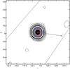 |
Fig. 21 Same as Fig. 8 but for Pal 1. The coordinates shown here are Galactic longitude and latitude. |
5.9. NGC 6205 (M 13)
NGC 6205 is currently at a distance of 8.2 kpc from the Galactic center, close to its perigalacticon Rperi = 5.0 kpc (D99). Thus, we expect potential tidal tails to be aligned with the orbital path. In Fig. 16 we show the resulting contour plot. The background shows residuals up to 2σ above the mean of 1.2 × 10⁻¹ stars arcmin-2. No large scale features are observed. The cluster’s central contours are smooth. The contours in the outer regions of the cluster show distortions. We detect a halo of extratidal stars with a slight elongation in the direction of motion. The number density profile in Fig. 6 reveals an overabundance of stars around the tidal radius. Leon et al. (2000) studied the 2D distribution of NGC 6205 as well. They also detected disturbed contours in the southeast, corresponding to the feature visible in our data.
5.10. NGC 6341 (M 92)
NGC 6341 is located 8.2 kpc away from the Sun, close to its apogalacticon, Rapo = 9.9 kpc (D99). In Fig. 17 we show our derived contours of NGC 6341. In the left panel the effect of missing data due to the boundary of the SDSS scan regions in the southeast corner is visible. Northeast of the cluster we detected an artificially doubled background density. We corrected for this. All stars in the area denoted by the dashed gray line were studied. If two stars were closer than 2″ and similar in color and magnitude one of the stars was deleted from the sample. As seen in the contour map in this way we were able to reach almost the same background level as in any other area of our contour map. The mean background level was determined in the area northeast and southwest of the cluster ignoring the spurious areas. The mean field background is 9.6 × 10⁻² stars arcmin-2. The background shows overdensities with contours of 3σ and more mainly southwest of the GC.
The zoom-in in the lower panel of the same figure reveals mostly smooth contours in the cluster center. The main distortion is in the direction of the corrected background and due to the missing data on the opposite side of the cluster it is not possible to say whether this feature indicates a tidal tail. But also along a southwest to northeast axis we detect extratidal material. The 2D structure of NGC 6341 has been studied before by Testa et al. (2000). They observed somewhat elongated contours in the same direction as we do. The number density profile in Fig. 6 shows an overabundance of stars around the tidal radius.
5.11. NGC 7006
NGC 7006 is one of the most remote clusters in our sample with a distance to the Galactic center of RMW = 38.8 kpc. The cluster is currently moving toward the Galactic plane and the Galactic center (Dinescu et al. 2001). It has not been included in any study on tidal tails searches so far. In Fig. 18 we show its contour map. We clearly detect the GC as the highest overdensity. The 1σ-contour is very distorted and comparable to the background noise. The mean field background level is 1.2 × 10⁻¹ stars arcmin-2. The 2σ and 3σ contours show some symmetric distortion. All higher contours are smooth, although the halo of extratidal stars for NGC 7006 is huge. For no other cluster in our sample we find such a large extratidal halo.
5.12. NGC 7078 (M15)
NGC 7078 is currently located 9.8 kpc from the Galactic center, close to its apogalacticon Rapo = 10.4 kpc (D99), i.e., we do not expect any correlation between the orbit and the (possible) tail’s orientation. In Fig. 19 we show the contour map. The field around the cluster is very smooth. It shows two peaks of 3σ above the mean of 3.0 × 10⁻¹ stars arcmin-2, but not in any symmetric configuration around the cluster. No large scale structures are detected. The contours at the cluster center are undisturbed, but the contours at the tidal radius show some distortions. The proximity of NGC 7078 to the edge of the SDSS survey introduces some asymmetry. Nevertheless, we observe an extratidal extension in southwestern direction. Grillmair et al. (1995) studied the 2D distribution of NGC 7078. They found an excess of cluster stars extending toward the southeast and a further density peak just north of the cluster. These features do not show up in our data. Instead, we confirm the features seen in the immediate surroundings of NGC 7078 that were also found by Chun et al. (2010). Owing to the borders of the SDSS survey, their northwestern feature is not covered by our data. On a larger scale, outside the field of view of Chun et al. (2010), we see extended low-density (1 − 2σ) structures in roughly east-west direction. These are not aligned with the direction toward the Galactic center, but appear at an angle of approximately 20 − 30deg (Fig. 19), suspiciously aligned with the direction of the SDSS scan. While suggestive, deeper data are needed to confirm or rule out whether these are extended tidal tails. We observe a similar extratidal structure of the contour lines. Fig. 6 shows the number density profile of NGC 7078. We detect a change in the profile’s slope.
5.13. NGC 7089 (M2)
NGC 7089 is located 10.1 kpc from the Galactic center, close to perigalacticon Rperi = 6.4 kpc (D99). I.e. a possible inner tidal tail is expected to be aligned with the orbital path of the cluster. In Fig. 20 we show the contour plot of NGC 7089. The inner contours are smooth. The extended 1σ-contour is comparable to the background contours. The overall background shows at most contours of 2σ. The mean background level is at 1.2 × 10⁻¹ stars arcmin-2. No large scale features are detected. NGC 7089 shows an extratidal halo, which is a spherical structure. No 𝒮-shape or elongation is observed. Also Grillmair et al. (1995) studied the 2D structure of NGC 7089. They found an excess of cluster stars extending along an E-W axis. In our contours only the 2σ-contours might show some elongation, but overall the halo is quite circular.
Dalessandro et al. (2009) derived a number density profile and also detected a slight excess of stars beyond the tidal radius compared to the best fit King model. Our number density profile is shown in Fig. 6. We detect a change in slope around the tidal radius as expected for a halo of extratidal stars.
5.14. Palomar 1
Pal 1 is not a typical GC. Its CMD is quite unusual. It has a populated main sequence, but hardly any stars on the red giant and the horizontal branch. This feature was noticed by Borissova & Spassova (1995), Rosenberg et al. (1998), and Sarajedini et al. (2007). Further, this cluster might be up to 8 Gyr younger(!) than a typical GC like 47 Tuc (Sarajedini et al. 2007). It is also discussed in the literature, whether Pal 1 is a member of the Monoceros stream/Canis Major dwarf (Crane et al. 2003; Forbes & Bridges 2010). It cannot be ruled out that Pal 1 is misclassified as a GC since objects of this young an age are usually considered open clusters. The low background density contour map shown in Fig. 21 is plotted in Galactic longitude and latitude (l, b) due to the cluster’s high declination. Although Pal 1 has a high destruction probability (GO97), mainly driven by disk and bulge shocks, it does not show any distortions of its contours, except for a large circular halo of extratidal stars (comparable to NGC 7006). In the field we see no density peaks. The number density profile is shown in Fig. 7. The profile drops outside of ~30 arcmin because the edge of the survey is reached. In summary we can say that we detect a symmetric overdensity at the position of Pal 1.
5.15. Palomar 3
Pal 3 is currently at a distance of RMW = 84.9 kpc, very close to perigalacticon Rperi = 82.5 kpc (D99). As this is the cluster’s closest approach to the Galaxy we do not expect to see any large signs of dissolution due to tidal shocks. Also the destruction rates derived by GO97 are low. In Fig. 22 we show the contour map of a large area centered on Pal 3. The cluster can clearly be detected as the strongest overdensity. Nevertheless, the background shows several pronounced overdensities. The highest overdensity at (153.5, − 1.5) is the signal of the dwarf spheroidal galaxy Sextans. The cluster’s contours look undisturbed. We observe a distortion of the contours towards the Galactic center, but no corresponding feature on the opposite side. Generally, Pal 3 has a large extratidal halo which shows a sharp edge. The number density profile is shown in Fig. 7. We note that owing to the sparseness of Pal 3’s CMD and its large distance deeper data are needed to investigate options such as a connection with Sextans.
5.16. Palomar 4
A density plot of Pal 4 and surroundings is shown in Fig. 23. We discover a large halo of extratidal stars. The 1σ-contour is stretching along towards the Galactic center, but only in one direction. The field around Pal 4 is showing strong overdensities of up to 10σ. These density peaks show steep edges and in the center broad plateaus. It is unclear where these features are coming from. Comparing these field peaks with the cluster’s tidal tail, hardly any difference can be seen. An interesting structure of the contour lines is visible at the cluster’s western edge.
Sohn et al. (2003) studied the 2D morphology of Pal 3 and Pal 4 using CFH12K wide-field photometry. For Pal 3 they detect some extensions in the direction towards the Galactic center and anti-center which are not more prominent than 1σ over the background. For Pal 4 they see a tail extending to the NW. In our data we do not observe such a feature. Pal 4 is the most distant cluster in our sample. Again, deeper data are needed to reveal the possible existence of tidal tails.
5.17. Palomar 14
In Fig. 24 we show the contour map of Pal 14. Martínez Delgado et al. (2004) studied the CMD of Pal 14 and compared it to the CMD of a region outside the cluster. They detected some hints for extratidal stars in a region of the CMD. We see smooth central contours and an extratidal halo. The field background shows some overdensities of up to 5σ above the mean which is 1.47 × 10⁻¹ stars arcmin-2. The 1σ and 2σ contours show an elongated distortion, comparable to the field background contours. The extratidal halo is spherical with some asymmetry towards the southeast. Whether this indicates the beginning of sparsely populated tidal tails remains unclear. Also for this GC, deeper data would be desirable in order to confirm this or to rule it out.
6. Discussion
6.1. Horizontal branch stars
From theoretical investigations and simulations (e.g., Baumgardt & Makino 2003) we know that preferentially stars of lower mass are lost. Measurements of the mass function of Pal 5 and its tidal tails confirm this picture (Koch et al. 2004). Also the number density of main sequence stars is larger than for RGB stars. Therefore, tracing tidal structures with only upper RGB stars may be difficult, as is the case for Pal 3, Pal 4, Pal 14 and NGC 2419 and this is exacerbated by the sparsely populated RGBs of the Palomar GCs. Nonetheless, we do find halos of extratidal stars as possible signs for some dissolution for all four clusters. But the field background is noisy and shows overdensities of more than 3σ.
The blue horizontal branch (BHB) and RR Lyrae stars are located at a position in the CMD where hardly any field stars are located. Therefore any BHB or RR Lyrae star at the cluster distance found outside the cluster’s tidal radius is with a high probability a former cluster member. For NGC 5466, Belokurov et al. (2006) found that the BHB/RR Lyrae stars also trace the tidal tails. For those of our GCs that show no long tidal structures, but only distorted tidal contours the majority of the BHB/RR Lyrae stars are inside the tidal radius. As an example: in NGC 6341, we found 194 BHB/RR Lyrae stars. Only 20 of those are found outside the tidal radius. The remaining 174 BHB/RR Lyrae stars are all found within the tidal radius (red ellipse in Fig. 17). For NGC 4147, for which we have found a complex multiple arm morphology and extended 1σ structures that look like weak tidal tails, most BHB stars are within the innermost drawn contour, and 30% are found outside. The BHB stars do not trace the multiple arms. But the BHB/RR Lyrae stars in the field are mostly found in overdensities. E.g., at (181.2, 17) two overdensities of 9σ and 10σ, respectively are found. In the center of both a single BHB/RR Lyrae star is detected. At the same time, there are BHB stars that are not connected to any overdensity. The algorithm used to derive the density of cluster member stars gives high weights to BHB and RR Lyrae stars. Without spectroscopic information it is not possible to draw any reliable conclusion whether BHB/RR Lyrae stars connected to a prominent overdensity in the background are “lost” cluster members. But the existence of BHB/RR Lyrae stars without any overdensity is supporting the hypothesis that the stars in those overdensities are more likely former member stars.
A similar connection between some of the cluster’s BHB/RR Lyrae stars and overdensities in the field is observed for NGC 5024, NGC 5053, NGC 5466, NGC 5904, NGC 6205, and NGC 7006. Our current data do not permit us to conclude whether these overdensities are related to the GCs.
For some GCs in our sample a connection to the Sagittarius stream (e.g., Bellazzini et al. 2003b; Law & Majewski 2010; Forbes & Bridges 2010) or the Monoceros stream (Crane et al. 2003; Forbes & Bridges 2010) is discussed in the literature. It is possible that the detected extratidal structures and overdensities in the field of NGC 4147, NGC 5024, NGC 5053 and Pal 1 are features induced by the field populations of the disrupted dwarf galaxies. The data used here do not allow us to make a definite conclusion.
6.2. Comparison to theory
The vital diagram of GO97 in Fig. 1 predicts a dissolution of NGC 4147 due to 2-body relaxation. The multiple arm feature observed in Fig. 9 for NGC 4147 supports the cluster’s dissolution. Furthermore, the simulations by Montuori et al. (2007) found such a multiple arm morphology for GCs on eccentric orbits approaching apocenter. NGC 4147’s current position close to apogalacticon matches the simulations well. Of all stars in the distorted 1σ-contour around NGC 4147 about 13% are found outside the 4σ-contour. The 4σ-contour corresponds roughly to the Jacobi radius of NGC 4147 (Baumgardt et al. 2010), i.e., stars outside the 4σ-contour left the potential field of the cluster. The tidal features of NGC 4147 are smaller than the ones for Pal 5. Pal 5 is close to destruction due to tidal shocks, while NGC 4147’s dissolution is mainly driven by relaxation.
The Palomar clusters in our sample also lie outside the triangles in Fig. 1. As the outermost triangle is only appropriate for clusters with a current distance to the Galactic center smaller than 12 kpc, and Pal 3, Pal 4, and Pal 14 are currently further than 69 kpc away from the Milky Way no conclusions can be drawn from the diagram for these three clusters. Pal 5 is known to have tidal tails. Its destruction rate was studied in detail by Dehnen et al. (2004).
Pal 1 is also located outside the triangles in the vital diagram. Hence a dissolution due to 2-body relaxation is likely, but the contour map in Fig. 21 shows no typical 𝒮-shape. It reveals a large, spherical extratidal halo though. The halo extends much further out than the cluster’s Jacobi radius. The Jacobi radius is slightly smaller than the 20σ-contour (the second most inner contour). 71% of all stars located within the 1σ-contour are found outside the Jacobi radius, i.e., should not be bound to the GC anymore. Pal 1 in general is an interesting object. Its CMD shows a clear main sequence but a very sparsely populated red giant branch. The low stellar density makes it difficult to detect tidal tails if present. The question of whether Pal 1 is really a GC or rather an open cluster remains unsolved.
The remaining GCs in our sample from the NGC catalog are all located well within the triangles of GO97’s vital diagram. Hence, no (pronounced) signs for dissolution are expected. NGC 5466 is an exception and shows that the theoretical calculations can be improved, as tidal tails have been detected. For NGC 5053 some contours are located outside the Jacobi radius, a possible sign for unbound cluster stars in the northeast, west, and southwest. Generally the clusters show an extratidal halo, which is to be expected from dynamical studies. These GCs are not in danger to be destroyed within the next Hubble time, according to GO97 and D99. This is supported by the lack of large scale tidal features in our study.
6.3. Number density profiles and halos of extratidal stars
Most of the clusters in our sample show a (pronounced) halo of stars outside the tidal boundary. Combes et al. (1999) simulated GCs in a tidal field and observed such a halo as well. The stars outside the tidal radius spread out in density like a power law. Combes et al. (1999) transformed the 3-dimensional simulations into a (observable) projection on the sky and derived the power law to be “r-3 or steeper”. The extratidal halos observed by Grillmair et al. (1995) and Leon et al. (2000) show only slopes of −1. Combes et al. (1999) argue that the discrepancy is a consequence of noisy background-foreground subtraction. Our stellar sample contains very little contamination. Therefore, an investigation of these halos is of interest. Furthermore, Grillmair et al. (1995) observed for clusters with tidal extensions a break in their number density profiles, becoming pure power laws at larger radii.
Leon et al. (2000) introduced
 as the slope of the number
density profile between a·rt and
b·rt. They chose to compute the three
slopes:
as the slope of the number
density profile between a·rt and
b·rt. They chose to compute the three
slopes:  ,
,  , and
, and  . We applied the same method to
the clusters in our sample and derived the three slopes. In the profiles shown in
Figs. 5–7
slope changes are visible in many clusters. The slope was only computable for
clusters, where the background was not too noisy. In order to fit the power law slopes we
performed a least-squares fit between the two radii. In Table 4 we list the resulting slopes for all clusters.
. We applied the same method to
the clusters in our sample and derived the three slopes. In the profiles shown in
Figs. 5–7
slope changes are visible in many clusters. The slope was only computable for
clusters, where the background was not too noisy. In order to fit the power law slopes we
performed a least-squares fit between the two radii. In Table 4 we list the resulting slopes for all clusters.
The theoretical prediction of slopes of “r-3 or steeper” is
observed for many clusters in our sample for . Only
NGC 4147, NGC 5053, Pal 4, and Pal 5 have a significantly flatter slope than predicted.
The measurement for Pal 3 is affected by a large error. The fits for
show large errors or were in
some cases not possible at all, due to the noisy background. For Pal 1, we did not perform
any fit due to the strange shape of the number density profile. In general, the simulated
halos of Combes et al. (1999) reproduce well the
observed halos.
Power law slopes of the radial density
profiles between the two radii a·rt and
b × rt.
For most GCs an extratidal halo exists, while the Jacobi radius is larger than this halo. This is the case for NGC 2419, NGC 5024, NGC 5272, NGC 5904, NGC 6205, NGC 6341, NGC 7006, NGC 7078, and NGC 7089. From the definition of the Jacobi radius this suggest that the stars in the extratidal halo have not left the cluster potential. The derivation of the Jacobi radius is based on measurements and assumptions, e.g., the mass-to-light ratio is assumed to be 2, which may not be generally true, see M05 for mass-to-light ratios of the Galactic GCs. One possibility is that the contour maps do not reveal halos of extratidal stars but just the halo of the GCs. Although, the simulations by Combes et al. (1999) reveal extratidal halos with the identical power-law slope as our observed halos.
The Palomar clusters have a halo of stars outside the Jacobi radius. Baumgardt et al. (2010) classifies these clusters as “tidally filled”. We actually observe that these clusters are even more extended. Pal 14 is a very special case: the Jacobi radius is smaller than the tidal radius from the King profile. The low measured velocity dispersion of Pal 14 does not suggest a dissolved GC (Jordi et al. 2009), neither do the mostly symmetrical contour lines. For Pal 5 the same observation is made, the Jacobi radius is smaller than the tidal radius. Pal 5 has a lower than expected velocity dispersion, although it will be destroyed within the next 110 Myr (Odenkirchen et al. 2002). It is possible that the large distance to Pal 14 prevents us from detecting its tidal tails although we do see possible extensions at the 1−2σ level. Or their orientation makes them difficult to detect. Simulations of dwarf spheroidals have shown that the detection of the characteristic 𝒮-shape of tidal tails depends on the position of the orbit relative to the line of sight (Muñoz et al. 2008).
7. Summary and conclusions
We studied the 2D distribution of (potential) member stars on the sky of the 17 GCs in the SDSS. The stars were chosen from the SDSS DR 7 and from An08. All stars in a field around a GC were selected in color and magnitude to match the observed colors and magnitudes of cluster stars.
We derived the number density profiles for the 17 clusters in our sample. Thanks to the large area coverage of the SDSS, we were able to trace the profiles as far out as to the flat field star background. In some cases a break in the profile was detected and interpreted as a sign for an extratidal halo. Comparing the profiles with the 2D distribution of cluster stars on the sky, we detected a halo of apparent extratidal stars for more clusters than a clear break in the profile.
A color–magnitude weighted counting algorithm from Odenkirchen et al. (2003) was used to derive density maps of cluster stars on the sky. We recovered the known extended tidal tails of Pal 5 and NGC 5466. For NGC 4147 we detected a complex, two arm feature of extratidal stars, and for NGC 5904 we find a roughly symmetric extension that might indicate short and stubby tails. For NGC 7006 and Pal 1 the extratidal halo is remarkably large. For Pal 1, 71% of the stars of the GCs are found outside the Jacobi radius, i.e., are not bound to the cluster anymore. Nevertheless, they are arranged spherically around the cluster. No sign of tidal effects is observed. We also detected extratidal features for NGC 5053, comparable to the findings of Lauchner et al. (2006). We confirm extratidal features in the immediate surroundings of NGC 7078 (Chun et al. 2010). For Pal 14 deeper data are needed in order to investigate whether the weakly visible extensions constitute tidal tails.
The comparison of our observations to the theoretical study of the GCs’ destruction rates by GO97 shows generally good agreement. Most NGC clusters in our sample were not expected to show signs for dissolution. They mostly only revealed a halo of extratidal stars well within their Jacobi radius. These extratidal halos show the theoretically expected “r-3” density slope for the majority of our sample.
Acknowledgments
K.J. would like to thank Shoko Jin for her help in deriving the direction of motion for each GC. We thank an anonymous referee for useful comments. K.J. and E.K.G. acknowledge support from the Swiss National Foundation through grant numbers 20020-122140 and 20020-113697. Funding for the SDSS and SDSS-II was provided by the Alfred P. Sloan Foundation, the Participating Institutions, the National Science Foundation, the US Department of Energy, the National Aeronautics and Space Administration, the Japanese Monbukagakusho, the Max Planck Society, and the Higher Education Funding Council for England. The SDSS was managed by the Astrophysical Research Consortium for the Participating Institutions. The Participating Institutions are American Museum of Natural History, Astrophysical Institute Potsdam, SEGUE and Supernovae, University of Basel, Cambridge University, Case Western Reserve University, University of Chicago, Drexel University, Fermi National Accelerator Laboratory, Institute for Advanced Study, Princeton Legacy, Japan Participation Group, Johns Hopkins University, Joint Institute for Nuclear Astrophysics, Kavli Institute for Particle Astrophysics and Cosmology, Korean Scientist Group, LAMOST, Los Alamos National Laboratory, Max-Planck-Institute for Astronomy/Heidelberg, Max-Planck-Institute for Astrophysics/Garching, New Mexico State University, Ohio State University, University of Pittsburgh, University of Portsmouth, Princeton University, US Naval Observatory, University of Washington.
References
- Abazajian, K. N., Adelman-McCarthy, J. K., Agüeros, M. A., et al. 2009, ApJS, 182, 543 [NASA ADS] [CrossRef] [Google Scholar]
- Adelman-McCarthy, J. K., Agüeros, M. A., Allam, S. S., et al. 2007, ApJS, 172, 634 [NASA ADS] [CrossRef] [Google Scholar]
- Allen, C., Moreno, E., & Pichardo, B. 2006, ApJ, 652, 1150 [NASA ADS] [CrossRef] [Google Scholar]
- An, D., Johnson, J. A., Clem, J. L., et al. 2008, ApJS, 179, 326 [NASA ADS] [CrossRef] [Google Scholar]
- Baumgardt, H., & Makino, J. 2003, MNRAS, 340, 227 [Google Scholar]
- Baumgardt, H., Parmentier, G., Gieles, M., & Vesperini, E. 2010, MNRAS, 401, 1832 [NASA ADS] [CrossRef] [Google Scholar]
- Bellazzini, M. 2007, A&A, 473, 171 [NASA ADS] [CrossRef] [EDP Sciences] [Google Scholar]
- Bellazzini, M., Ferraro, F. R., & Ibata, R. 2003a, AJ, 125, 188 [NASA ADS] [CrossRef] [Google Scholar]
- Bellazzini, M., Ibata, R., Ferraro, F. R., & Testa, V. 2003b, A&A, 405, 577 [NASA ADS] [CrossRef] [EDP Sciences] [Google Scholar]
- Belokurov, V., Evans, N. W., Irwin, M. J., Hewett, P. C., & Wilkinson, M. I. 2006, ApJ, 637, L29 [NASA ADS] [CrossRef] [Google Scholar]
- Borissova, J., & Spassova, N. 1995, A&AS, 110, 1 [Google Scholar]
- Capuzzo Dolcetta, R., Di Matteo, P., & Miocchi, P. 2005, AJ, 129, 1906 [NASA ADS] [CrossRef] [Google Scholar]
- Casetti-Dinescu, D. I., Girard, T. M., Majewski, S. R., et al. 2009, ApJ, 701, L29 [NASA ADS] [CrossRef] [Google Scholar]
- Chun, S., Kim, J., Sohn, S. T., et al. 2010, AJ, 139, 606 [NASA ADS] [CrossRef] [Google Scholar]
- Combes, F., Leon, S., & Meylan, G. 1999, A&A, 352, 149 [NASA ADS] [Google Scholar]
- Crane, J. D., Majewski, S. R., Rocha-Pinto, H. J., et al. 2003, ApJ, 594, L119 [NASA ADS] [CrossRef] [Google Scholar]
- Dalessandro, E., Beccari, G., Lanzoni, B., et al. 2009, ApJS, 182, 509 [NASA ADS] [CrossRef] [Google Scholar]
- Dehnen, W., Odenkirchen, M., Grebel, E. K., & Rix, H. 2004, AJ, 127, 2753 [NASA ADS] [CrossRef] [Google Scholar]
- Dinescu, D. I., Girard, T. M., & van Altena, W. F. 1999, AJ, 117, 1792 [NASA ADS] [CrossRef] [Google Scholar]
- Dinescu, D. I., Majewski, S. R., Girard, T. M., & Cudworth, K. M. 2001, AJ, 122, 1916 [NASA ADS] [CrossRef] [Google Scholar]
- Fellhauer, M., Evans, N. W., Belokurov, V., Wilkinson, M. I., & Gilmore, G. 2007, MNRAS, 380, 749 [NASA ADS] [CrossRef] [Google Scholar]
- Forbes, D. A., & Bridges, T. 2010, MNRAS, 404, 1203 [NASA ADS] [Google Scholar]
- Fukugita, M., Ichikawa, T., Gunn, J. E., et al. 1996, AJ, 111, 1748 [NASA ADS] [CrossRef] [Google Scholar]
- Geyer, M. P., & Burkert, A. 2001, MNRAS, 323, 988 [NASA ADS] [CrossRef] [Google Scholar]
- Gnedin, O. Y., & Ostriker, J. P. 1997, ApJ, 474, 223 [NASA ADS] [CrossRef] [Google Scholar]
- Grillmair, C. J., & Dionatos, O. 2006, ApJ, 641, L37 [NASA ADS] [CrossRef] [Google Scholar]
- Grillmair, C. J., & Johnson, R. 2006, ApJ, 639, L17 [NASA ADS] [CrossRef] [Google Scholar]
- Grillmair, C. J., Freeman, K. C., Irwin, M., & Quinn, P. J. 1995, AJ, 109, 2553 [NASA ADS] [CrossRef] [Google Scholar]
- Gunn, J. E., Carr, M., Rockosi, C., et al. 1998, AJ, 116, 3040 [NASA ADS] [CrossRef] [Google Scholar]
- Gunn, J. E., Siegmund, W. A., Mannery, E. J., et al. 2006, AJ, 131, 2332 [NASA ADS] [CrossRef] [Google Scholar]
- Harris, W. E. 1996, AJ, 112, 1487 [NASA ADS] [CrossRef] [Google Scholar]
- Hilker, M. 2006, A&A, 448, 171 [NASA ADS] [CrossRef] [EDP Sciences] [Google Scholar]
- Hogg, D. W., Finkbeiner, D. P., Schlegel, D. J., & Gunn, J. E. 2001, AJ, 122, 2129 [NASA ADS] [CrossRef] [Google Scholar]
- Ivezić, Ž., Lupton, R. H., Schlegel, D., et al. 2004, Astron. Nachr., 325, 583 [NASA ADS] [CrossRef] [Google Scholar]
- Ivezić, Ž., Smith, J. A., Miknaitis, G., et al. 2007, AJ, 134, 973 [NASA ADS] [CrossRef] [Google Scholar]
- Jordi, K., Grebel, E. K., Hilker, M., et al. 2009, AJ, 137, 4586 [NASA ADS] [CrossRef] [Google Scholar]
- Just, A., Berczik, P., Petrov, M. I., & Ernst, A. 2009, MNRAS, 392, 969 [NASA ADS] [CrossRef] [Google Scholar]
- King, I. 1962, AJ, 67, 471 [NASA ADS] [CrossRef] [Google Scholar]
- Kiss, L. L., Székely, P., Bedding, T. R., Bakos, G. Á., & Lewis, G. F. 2007, ApJ, 659, L129 [NASA ADS] [CrossRef] [Google Scholar]
- Koch, A., Grebel, E. K., Odenkirchen, M., Martínez-Delgado, D., & Caldwell, J. A. R. 2004, AJ, 128, 2274 [NASA ADS] [CrossRef] [Google Scholar]
- Kroupa, P. 2001, MNRAS, 322, 231 [NASA ADS] [CrossRef] [Google Scholar]
- Küpper, A. H. W., MacLeod, A., & Heggie, D. C. 2008, MNRAS, 387, 1248 [NASA ADS] [CrossRef] [Google Scholar]
- Küpper, A. H. W., Kroupa, P., Baumgardt, H., & Heggie, D. C. 2010, MNRAS, 401, 105 [NASA ADS] [CrossRef] [Google Scholar]
- Lauchner, A., Powell, Jr., W. L., & Wilhelm, R. 2006, ApJ, 651, L33 [NASA ADS] [CrossRef] [Google Scholar]
- Law, D. R., & Majewski, S. R. 2010, ApJ, 718, 1128 [NASA ADS] [CrossRef] [Google Scholar]
- Lehmann, I., & Scholz, R. 1997, A&A, 320, 776 [NASA ADS] [Google Scholar]
- Leon, S., Meylan, G., & Combes, F. 2000, A&A, 359, 907 [NASA ADS] [Google Scholar]
- Lupton, R. H., Ivezic, Z., Gunn, J. E., et al. 2002, in Society of Photo-Optical Instrumentation Engineers (SPIE) Conf. Ser., ed. J. A. Tyson, & S. Wolff, 4836, 350 [Google Scholar]
- Martell, S. L., & Grebel, E. K. 2010, A&A, 519, A14 [NASA ADS] [CrossRef] [EDP Sciences] [Google Scholar]
- Martínez Delgado, D., Dinescu, D. I., Zinn, R., et al. 2004, in Satellites and Tidal Streams, ed. F. Prada, D. Martinez Delgado, & T. J. Mahoney, ASP Conf. Ser., 327, 255 [Google Scholar]
- McLaughlin, D. E., & van der Marel, R. P. 2005, ApJS, 161, 304 [NASA ADS] [CrossRef] [Google Scholar]
- Montuori, M., Capuzzo-Dolcetta, R., Di Matteo, P., Lepinette, A., & Miocchi, P. 2007, ApJ, 659, 1212 [NASA ADS] [CrossRef] [Google Scholar]
- Muñoz, R. R., Majewski, S. R., & Johnston, K. V. 2008, ApJ, 679, 346 [NASA ADS] [CrossRef] [Google Scholar]
- Noyola, E., & Gebhardt, K. 2006, AJ, 132, 447 [NASA ADS] [CrossRef] [Google Scholar]
- Odenkirchen, M., & Grebel, E. K. 2004, in Satellites and Tidal Streams, ed. F. Prada, D. Martinez Delgado, & T. J. Mahoney, ASP Conf. Ser., 327, 284 [Google Scholar]
- Odenkirchen, M., Brosche, P., Geffert, M., & Tucholke, H. 1997, New A, 2, 477 [Google Scholar]
- Odenkirchen, M., Grebel, E. K., Rockosi, C. M., et al. 2001, ApJ, 548, L165 [NASA ADS] [CrossRef] [Google Scholar]
- Odenkirchen, M., Grebel, E. K., Dehnen, W., Rix, H., & Cudworth, K. M. 2002, AJ, 124, 1497 [NASA ADS] [CrossRef] [Google Scholar]
- Odenkirchen, M., Grebel, E. K., Dehnen, W., et al. 2003, AJ, 126, 2385 [NASA ADS] [CrossRef] [Google Scholar]
- Odenkirchen, M., Grebel, E. K., Kayser, A., Rix, H., & Dehnen, W. 2009, AJ, 137, 3378 [NASA ADS] [CrossRef] [Google Scholar]
- Peñarrubia, J., Navarro, J. F., McConnachie, A. W., & Martin, N. F. 2009, ApJ, 698, 222 [NASA ADS] [CrossRef] [Google Scholar]
- Pier, J. R., Munn, J. A., Hindsley, R. B., et al. 2003, AJ, 125, 1559 [NASA ADS] [CrossRef] [Google Scholar]
- Plummer, H. C. 1911, MNRAS, 71, 460 [CrossRef] [Google Scholar]
- Rockosi, C. M., Odenkirchen, M., Grebel, E. K., et al. 2002, AJ, 124, 349 [NASA ADS] [CrossRef] [Google Scholar]
- Rosenberg, A., Saviane, I., Piotto, G., Aparicio, A., & Zaggia, S. R. 1998, AJ, 115, 648 [NASA ADS] [CrossRef] [Google Scholar]
- Sarajedini, A., Bedin, L. R., Chaboyer, B., et al. 2007, AJ, 133, 1658 [NASA ADS] [CrossRef] [Google Scholar]
- Schlegel, D. J., Finkbeiner, D. P., & Davis, M. 1998, ApJ, 500, 525 [NASA ADS] [CrossRef] [Google Scholar]
- Schneider, D. P., Hall, P. B., Richards, G. T., et al. 2007, AJ, 134, 102 [NASA ADS] [CrossRef] [Google Scholar]
- Smith, J. A., Tucker, D. L., Kent, S., et al. 2002, AJ, 123, 2121 [Google Scholar]
- Sohn, Y., Park, J., Rey, S., et al. 2003, AJ, 126, 803 [NASA ADS] [CrossRef] [Google Scholar]
- Testa, V., Zaggia, S. R., Andreon, S., et al. 2000, A&A, 356, 127 [NASA ADS] [Google Scholar]
- Trager, S. C., King, I. R., & Djorgovski, S. 1995, AJ, 109, 218 [NASA ADS] [CrossRef] [Google Scholar]
- Tucker, D. L., Kent, S., Richmond, M. W., et al. 2006, Astron. Nachr., 327, 821 [NASA ADS] [CrossRef] [Google Scholar]
- Vivas, A. K., & Zinn, R. 2006, AJ, 132, 714 [NASA ADS] [CrossRef] [Google Scholar]
- Willman, B., Masjedi, M., Hogg, D. W., et al. 2006, unpublished, [arXiv:astro-ph/0603486] [Google Scholar]
- York, D. G., Adelman, J., Anderson, Jr., J. E., et al. 2000, AJ, 120, 1579 [Google Scholar]
All Tables
Power law slopes of the radial density
profiles between the two radii a·rt and
b × rt.
All Figures
|
Fig. 1 Vital diagram from GO97. The red stars are the GCs in our sample. Cluster mass and half-light radius were taken from GO97. GCs within the triangles are most likely surviving the next Hubble time. Adopted from G097, reproduced by permission of the AAS. |
| In the text | |
|
Fig. 2 Top rows: color–magnitude diagrams of all GCs in our sample in order of increasing distance from the Sun. The distances from Harris (1996) are printed in each CMD. The gray horizontal line marks the magnitude limit for each cluster. Bottom rows: color–magnitude diagrams of a random field in the vicinity of the cluster (see text for details). |
| In the text | |
|
Fig. 3 Color magnitude diagrams (c1,g) and (c2,g). Plotted are stars of NGC 6341 within one third of the cluster’s tidal radius. The gray solid lines denote the borders within which the stars were selected. |
| In the text | |
|
Fig. 4 Hess diagrams of the field (left panel) and cluster (right panel) sample of NGC 5272. Only stars already selected in c1 and c2 were used. |
| In the text | |
|
Fig. 5 Number density profiles of NGC 2419, NGC 4147, NGC 5024, NGC 5053, NGC 5272, and NGC 5466. The black open squares show the combined profiles. The black filled squares were derived in this study. The light gray solid line is the best fit King profile. The dark gray line is the best fit Plummer profile. The horizontal line marks the measured, mean background nbkg. |
| In the text | |
|
Fig. 6 Number density profiles of NGC 5904, NGC 6205, NGC 6341, NGC 7006, NGC 7078, and NGC 7089. The black open squares show the combined profiles. The black filled squares were derived in this study. The light gray solid line is the best fit King profile. The dark gray line is the best fit Plummer profile. The horizontal line marks the measured, mean background nbkg. |
| In the text | |
|
Fig. 7 Number density profiles of Pal 1, Pal 3, Pal 4, Pal 5, and Pal 14. The black open squares show the combined profiles. The black filled squares were derived in this study. The light gray solid line is the best fit King profile. The dark gray line is the best fit Plummer profile. The horizontal line marks the measured, mean background nbkg. |
| In the text | |
|
Fig. 8 Left panel: contour plot of a large area centered on NGC 2419. Right panel: blow-up of the contour plot centered on NGC 2419. In both panels the isodensity lines are drawn at levels of 1,2,3,5,7,8,10,20,40,····σbkg above the mean weighted background level. The 1σbkg and 2σbkg contours are drawn in light gray, the higher levels are drawn in black. The solid gray arrow points towards the Galactic Center. The gray solid line marks the edge of the SDSS survey area. The red solid circle shows the King tidal radius. The blue dashed circle shows the Jacobi radius. |
| In the text | |
|
Fig. 9 Same as Fig. 8 but for NGC 4147. The gray dashed arrow indicates the direction of its Galactic motion based on the proper motions stated in Table 1. |
| In the text | |
|
Fig. 10 Same as Fig. 8 but for NGC 5024. The high overdensity in the left panel at (199, 17.8) is the GC NGC 5053. The solid black line denotes the area observed by Chun et al. (2010). |
| In the text | |
|
Fig. 11 Same as Fig. 8 but for NGC 5053. The high overdensity in the left panel at (198, 18) is the GC NGC 5024. |
| In the text | |
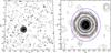 |
Fig. 12 Same as Fig. 8 but for NGC 5272. |
| In the text | |
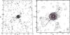 |
Fig. 13 Same as Fig. 8 but for NGC 5466. |
| In the text | |
|
Fig. 14 Same as Fig. 8 but for Pal 5. The overdensity at (229.5, 2) in the upper panel is the GC NGC 5904. |
| In the text | |
|
Fig. 15 Same as Figure 8 but for NGC 5904. The overdensity at (229,0) in the left panel is the GC Pal 5. |
| In the text | |
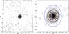 |
Fig. 16 Same as Fig. 8 but for NGC 6205. |
| In the text | |
|
Fig. 17 Same as Fig. 8 but for NGC 6341. The solid gray lines denote the edge of the SDSS footprint. The dashed gray line marks the area where the stellar density was doubled (see text for details). |
| In the text | |
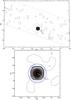 |
Fig. 18 Same as Fig. 8 but for NGC 7006. The solid gray lines denote the edge of the SDSS footprint. |
| In the text | |
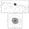 |
Fig. 19 Same as Fig. 8 but for NGC 7078. The solid gray lines denote the edge of the SDSS footprint. |
| In the text | |
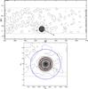 |
Fig. 20 Same as Fig. 8 but for NGC 7089. The solid gray lines denote the edge of the SDSS footprint. |
| In the text | |
|
Fig. 21 Same as Fig. 8 but for Pal 1. The coordinates shown here are Galactic longitude and latitude. |
| In the text | |
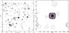 |
Fig. 22 Same as Fig. 8 but for Pal 3. |
| In the text | |
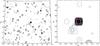 |
Fig. 23 Same as Fig. 8 but for Pal 4. |
| In the text | |
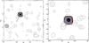 |
Fig. 24 Same as Fig. 8 but for Pal 14. |
| In the text | |
Current usage metrics show cumulative count of Article Views (full-text article views including HTML views, PDF and ePub downloads, according to the available data) and Abstracts Views on Vision4Press platform.
Data correspond to usage on the plateform after 2015. The current usage metrics is available 48-96 hours after online publication and is updated daily on week days.
Initial download of the metrics may take a while.