| Issue |
A&A
Volume 522, November 2010
|
|
|---|---|---|
| Article Number | A87 | |
| Number of page(s) | 8 | |
| Section | Numerical methods and codes | |
| DOI | https://doi.org/10.1051/0004-6361/201014345 | |
| Published online | 05 November 2010 | |
An absorbing boundary formulation for the stratified, linearized, ideal MHD equations based on an unsplit, convolutional perfectly matched layer
1
Max-Planck-Institut für Sonnensystemforschung,
Max Planck
Stra β e 2,
37191
Katlenburg-Lindau,
Germany
e-mail: This email address is being protected from spambots. You need JavaScript enabled to view it.
2
Department of Geosciences, Princeton University,
Princeton, NJ
08544,
USA
3
Université de Pau et des Pays de l’Adour, CNRS & INRIA
Magique-3D, Laboratoire de Modélisation et d’Imagerie en Géosciences UMR 5212, Avenue
de l’Université, 64013
Pau Cedex,
France
4
Institut universitaire de France, 103 boulevard Saint-Michel, 75005
Paris,
France
Received:
3
March
2010
Accepted:
29
July
2010
Abstract
Perfectly matched layers are a very efficient way to absorb waves on the outer edges of media. We present a stable convolutional unsplit perfectly matched formulation designed for the linearized stratified Euler equations. The technique as applied to the Magneto-hydrodynamic (MHD) equations requires the use of a sponge, which, despite placing the perfectly matched status in question, is still highly efficient at absorbing outgoing waves. We study solutions of the equations in the backdrop of models of linearized wave propagation in the Sun. We test the numerical stability of the schemes by integrating the equations over a large number of wave periods.
Key words: magnetohydrodynamics / Sun: helioseismology / waves / Sun: oscillations / methods: numerical
© ESO, 2010
1. Introduction
The choice of appropriate boundary conditions in simulations remains a significant challenge in computational physics. Amidst the vast number of options that exist, a widely invoked construct is that of the absorbing boundary, one that is expected to relieve the computational domain of outgoing waves or other structures without affecting the solution in the region of interest (for a review, see e.g., Colonius 2004). A number of different methods exist to accomplish this, such as an attenuating “sponge” (e.g., Lui 2003; Colonius 2004), characteristics-based boundary conditions (e.g. Thompson 1990), an artificially imposed supersonic outward directed advective flow (e.g., Lui 2003), perfectly matched layers (PMLs; Bérenger 1994), etc. Unfortunately, a number of these methods is afflicted with disadvantages, a primary cause of concern being that of absorption efficiency. For example, the characteristics-based boundary conditions do not perform very well when the incident waves at the boundary are significantly inclined – and a fair degree of reflection is observed. The sponges are better at absorbing the waves and are relatively easy to implement; however, the reflectivity can still be substantial.
The criterion of low reflectivity is perhaps best satisfied by the PML formulation, developed first by Bérenger (1994) as an absorbing layer for the Maxwell equations. The central idea of this technique lies in performing an analytic continuation of the wave vector into the complex plane. Wave vectors perpendicular to the boundary are forced to assume a decaying form in the complex plane, thereby dramatically reducing the amplitudes of the waves in the boundary PML region. In the absence of discretization errors, the PML as set out by Bérenger (1994) is highly absorbent. After numerical discretization however, there are weak associated reflections. An important issue in the classical split formulation of Bérenger (1994) is that the absorption efficiency decreases rapidly at grazing incidence (e.g., Collino & Monk 1998; Winton & Rappaport 2000).
There have been numerous advances in constructing stable analytic continuations of wave vectors in the boundary region. In particular, the stable convolutional PMLs (C-PML; e.g., Roden & Gedney 2000; Festa & Vilotte 2005; Komatitsch & Martin 2007; Drossaert & Giannopoulos 2007), contain a Butterworth filter inside the PML, thereby dramatically improving the absorption efficiency at grazing incidence. This formalism was adopted to the study of waves in anisotropic geophysical media by Komatitsch & Martin (2007); the numerical stability of said technique was studied by Komatitsch & Martin (2007); )Meza-Fajardo & Papageorgiou (2008). Extensions to the poro- and viscoelastic cases have been introduced by Martin et al. (2008) and Martin & Komatitsch (2009), respectively. Our goal in this contribution is to develop a C-PML for the 3D linearized ideal MHD equations in stratified media.
Astrophysical media such as stellar interiors and atmospheres may be strongly stratified and highly magnetized. Simulating wave propagation in such environments is of interest because in understanding the effects of stratification and magnetic fields on the oscillations, we may be able to better interpret observations and constrain certain properties of the object in question. In particular, we focus on the Sun, a star that has been well studied and for which high-quality observations exist. The interior of the Sun is opaque to electromagnetic waves – consequently, only photons that arrive from very close to the surface (photosphere) of the Sun are visible. Helioseismology is the inference of the internal structure and dynamics of the Sun by observing the surface manifestation of its acoustic pulsations (e.g., Christensen-Dalsgaard 2002; Gizon & Birch 2005; Gizon et al. 2010). Armed with accurate interaction theories of waves and measurements of the acoustic field at the surface, one can attempt to determine the sub-surface structure and dynamics of various solar features such as sunspots (see e.g., Gizon et al. 2009), large-scale meridional flow, interior convective length scales, etc. In order to construct these interaction theories, it is important to simulate and study small amplitude (linear) wave propagation in a solar-like medium – filled with scatterers like sunspots or mean flows. The time scales of wave propagation are typically much smaller than the rate at which the scatterer itself evolves; thus one may invoke the assumption of time stationarity of the background medium. Numerical simulations of waves in solar-like media have been performed by numerous groups (e.g., Werne et al. 2004; Hanasoge et al. 2006; Shelyag et al. 2006; Khomenko & Collados 2006; Cameron et al. 2007; Parchevsky & Kosovichev 2007; Hanasoge et al. 2008; Hanasoge 2008; Cameron et al. 2008). Two groups in particular (Khomenko & Collados 2006; Parchevsky & Kosovichev 2007) currently utilize the classical split PML formulation in order to solve the wave equations in stratified media. There exist drawbacks in these formulations. For example, Khomenko & Collados (2006) have noted that there are long term instabilities associated with their method. The technique discussed in Parchevsky & Kosovichev (2007) involves the addition of a small arbitrary constant (see Eq. (21) and related discussion of their article) that could possibly be acting as a sponge; it is unclear if their method is perfectly matched after the introduction of this constant. The modal power spectrum that Parchevsky & Kosovichev (2007) display in Fig. 9 of their article shows substantial reflected power from their lower boundary, atypical of perfectly matched formulations.
The plan of this article is as follows: in Sect. 2, we recall the linearized ideal MHD equations and discuss the C-PML method as was previously developed for the seismic wave equations. The C-PML is then extended to the stratified Euler/MHD equations in Sect. 3 and results from numerical tests are discussed. We summarize and conclude in Sect. 4.
2. The linearized ideal MHD equations
As discussed in the introduction, we consider a system with a steady background, the wave
equations are written as small perturbations around this state. The assumption of small
amplitude wave perturbations is consistent with observations of solar and stellar
oscillations (e.g., Christensen–Dalsgaard 2003; Bogdan 2000). In the equations that follow, all quantities
with a subscript “0” denote the steady background properties while the unsubscripted terms
represent the fluctuations around the corresponding property. All bold faced terms represent
vectors. ![Mathematical equation: \begin{eqnarray} \partial_t\rho &=& -\bnabla\dotp(\rho_0 \bbv), \label{cont.1}\\ \partial_t(\rho_0 \bbv) &=& \bnabla\cdot \left[\frac{\bB\bB_0}{4\pi} + \frac{\bB_0\bB}{4\pi} -\left(p + \frac{\bB_0\cdot\bB}{4\pi}\right)\underbar{\vec{I}}\right] - \rho{g_0}\ez \nonumber\\ &\quad +& \vec{S}(x,y,z,t), \label{mom.1}\\ \partial_t p &=& -c_0^2\rho_0\bnabla\dotp\bbv - \bbv\dotp\bnabla p_0,\label{press.1}\\ \partial_t \bB &=& \bnabla\cdot\left( \bB_0\bbv- \bbv\bB_0\right),\label{ind.1}\\ \bnabla\cdot\bB &=& 0\cdot \label{div.1} \end{eqnarray}](/articles/aa/full_html/2010/14/aa14345-10/aa14345-10-eq2.png) In
order, these are the equations of continuity (Eq. (1)), momentum (Eq. 2)),
adiabaticity (Eq. (3)), induction (Eq. (4)), and divergence-free field (Eq. (5)). The terms ρ and
p denote density and pressure,
B = (Bx,By,Bz)
is the magnetic field, g0 is the gravity,
c0 the sound speed, and
v = (vx,vy,vz)
is the velocity. A Cartesian coordinate system (x,y,z) with unit vectors
(ex,ey,ez)
is adopted. The identity tensor is
In
order, these are the equations of continuity (Eq. (1)), momentum (Eq. 2)),
adiabaticity (Eq. (3)), induction (Eq. (4)), and divergence-free field (Eq. (5)). The terms ρ and
p denote density and pressure,
B = (Bx,By,Bz)
is the magnetic field, g0 is the gravity,
c0 the sound speed, and
v = (vx,vy,vz)
is the velocity. A Cartesian coordinate system (x,y,z) with unit vectors
(ex,ey,ez)
is adopted. The identity tensor is  . The momentum equations are forced by
an arbitrary spatio-temporally smooth source function S. All
background terms
p0,ρ0,c,B0
are assumed to be heterogeneous, i.e., functions of (x,y,z) and
g0 = g0(z). Note
that we have assumed the background medium to be non-moving, i.e., that
v0 = 0. The extension to the
v0 ≠ 0 situation requires no additional
treatment at the boundary as long as the background velocity is zero in this region.
. The momentum equations are forced by
an arbitrary spatio-temporally smooth source function S. All
background terms
p0,ρ0,c,B0
are assumed to be heterogeneous, i.e., functions of (x,y,z) and
g0 = g0(z). Note
that we have assumed the background medium to be non-moving, i.e., that
v0 = 0. The extension to the
v0 ≠ 0 situation requires no additional
treatment at the boundary as long as the background velocity is zero in this region.
2.1. PMLs and C-PMLs
Consider a wave propagating in the z direction, towards the upper
boundary. For now, ignoring the fact that the medium is stratified, we have
vz ~ Aei(kzz − ωt),
where A is the amplitude of the wave,
kz is the wavenumber along the vertical
direction, ω the frequency, and t, time. The classical
PML of Bérenger (1994) prescribes the following
transformation for kz: ![Mathematical equation: \begin{equation} k_z \rightarrow {k_z}\left[{1 - \frac{d}{i\omega}}\right], \label{pml.classic} \end{equation}](/articles/aa/full_html/2010/14/aa14345-10/aa14345-10-eq23.png) (6)where
d = d(z)f(x,y,z0) ≥ 0
is a damping parameter and z = z0 is the
vertical coordinate corresponding to the entrance of the layer. We include the term
f(x,y,z0) to account for
the possibility of strong wave speed variations in the horizontal (non-PML) directions at
z = z0 (i.e., at the entrance of the PML).
Note that the damping term applies only to
kz; i.e. the wavenumbers
kx and
ky remain unchanged. It has been shown
that, cast in the form of Eq. (6), the PML
is unstable in a number of situations (for
f(x,y,z0) = 1), including
in the presence of mean flows (e.g., Hu 2001; Appelö et al. 2006), and in anisotropic media (e.g.,
Bécache et al. 2003; Komatitsch & Martin 2007, also personal communication, Khomenko
2009). A version of the PML with a more general transformation was introduced by Roden & Gedney (2000) for Maxwell equations and
adapted to the seismic wave equation by Festa &
Vilotte (2005), Komatitsch & Martin
(2007), and Drossaert & Giannopoulos
(2007). They applied the following relation:
(6)where
d = d(z)f(x,y,z0) ≥ 0
is a damping parameter and z = z0 is the
vertical coordinate corresponding to the entrance of the layer. We include the term
f(x,y,z0) to account for
the possibility of strong wave speed variations in the horizontal (non-PML) directions at
z = z0 (i.e., at the entrance of the PML).
Note that the damping term applies only to
kz; i.e. the wavenumbers
kx and
ky remain unchanged. It has been shown
that, cast in the form of Eq. (6), the PML
is unstable in a number of situations (for
f(x,y,z0) = 1), including
in the presence of mean flows (e.g., Hu 2001; Appelö et al. 2006), and in anisotropic media (e.g.,
Bécache et al. 2003; Komatitsch & Martin 2007, also personal communication, Khomenko
2009). A version of the PML with a more general transformation was introduced by Roden & Gedney (2000) for Maxwell equations and
adapted to the seismic wave equation by Festa &
Vilotte (2005), Komatitsch & Martin
(2007), and Drossaert & Giannopoulos
(2007). They applied the following relation: ![Mathematical equation: \begin{equation} k_z \rightarrow {k_z}\left[{\kappa + \frac{d}{\alpha - i\omega}}\right]\label{wave.trans1}, \end{equation}](/articles/aa/full_html/2010/14/aa14345-10/aa14345-10-eq31.png) (7)where
α = α(z) > 0 and
κ = κ(z) ≥ 1 are additional
parameters. In particular, the inclusion of α, i.e. of a filter, helped
improve the issue of damping waves with grazing incidence at the boundaries. We follow the
formalism set out in Komatitsch & Martin
(2007) and derive the equations for the convolutional PML. The transformation of
Eq. (7) corresponds to a grid stretching
of the relevant coordinate:
(7)where
α = α(z) > 0 and
κ = κ(z) ≥ 1 are additional
parameters. In particular, the inclusion of α, i.e. of a filter, helped
improve the issue of damping waves with grazing incidence at the boundaries. We follow the
formalism set out in Komatitsch & Martin
(2007) and derive the equations for the convolutional PML. The transformation of
Eq. (7) corresponds to a grid stretching
of the relevant coordinate:  (8)Derivatives along
the vertical direction in Eqs. (1)
through (5) are now computed in terms of
the stretched coordinate. In other words, the vertical derivative of a generic variable
ψ(x,y,z,t) is transformed according to:
(8)Derivatives along
the vertical direction in Eqs. (1)
through (5) are now computed in terms of
the stretched coordinate. In other words, the vertical derivative of a generic variable
ψ(x,y,z,t) is transformed according to:
 (9)The term
 may be rewritten as:
![Mathematical equation: \begin{eqnarray} \partial_{\tz}\psi &=& \left[\frac{1}{\kappa} - \frac{d/\kappa^2}{ (d/\kappa + \alpha)-i\omega }\right] \partial_z\psi. \label{wave.trans2} \end{eqnarray}](/articles/aa/full_html/2010/14/aa14345-10/aa14345-10-eq39.png) (10)The
first term inside the parenthesis on the right-hand side of Eq. (10) is easily obtained by dividing the
derivative by κ. The second term is more complicated because it involves
products in the temporal Fourier space of two terms with frequency content; this results
in a convolution in time. In order to compute these convolutions, Roden & Gedney (2000); ); )Festa & Vilotte (2005); )Komatitsch
& Martin (2007) use a recursion formula to update the convolution at each
time step. Instead of applying a recursive relation, here we use a differential equation
to recover
(10)The
first term inside the parenthesis on the right-hand side of Eq. (10) is easily obtained by dividing the
derivative by κ. The second term is more complicated because it involves
products in the temporal Fourier space of two terms with frequency content; this results
in a convolution in time. In order to compute these convolutions, Roden & Gedney (2000); ); )Festa & Vilotte (2005); )Komatitsch
& Martin (2007) use a recursion formula to update the convolution at each
time step. Instead of applying a recursive relation, here we use a differential equation
to recover  (also done in the auxiliary differential
equation formulation of Gedney & Zhao 2010;
Martin et al. 2010), where
(also done in the auxiliary differential
equation formulation of Gedney & Zhao 2010;
Martin et al. 2010), where
 (11)Let the time history of
χ be such that χ(x,y,z,t ≤ 0) = 0. In
addition, we also require
∂zψ = 0 for all
t ≤ 0. Then, the following differential equation
for χ
(11)Let the time history of
χ be such that χ(x,y,z,t ≤ 0) = 0. In
addition, we also require
∂zψ = 0 for all
t ≤ 0. Then, the following differential equation
for χ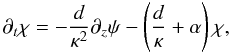 (12)ensures that
χ has the desired frequency response, i.e.,
(12)ensures that
χ has the desired frequency response, i.e.,
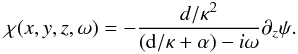 (13)The differential
equations for the C-PML may now be written as:
(13)The differential
equations for the C-PML may now be written as: ![Mathematical equation: \begin{eqnarray} \partial_t\rho &=& -\bnabla_h\dotp(\rho_0 \bbv) - \rho_0\partial_{\tz}v_z - v_z\partial_{\tz} \rho_0,\label{mod.cont}\\ \partial_t \left(\rho_0\bbv\right) &=& \bnabla_h\cdot \left[\frac{\bB\bB_0}{4\pi} + \frac{\bB_0\bB}{4\pi} -\left(p + \frac{\bB_0\cdot\bB}{4\pi}\right)\vec{I}\right] \nonumber\\ &\quad +& \partial_{\tz}\left[\frac{B_z\bB_0}{4\pi} + \frac{B_{0z}\bB}{4\pi} -\left(p + \frac{\bB_0\cdot\bB}{4\pi}\right)\ez\right] \nonumber\\ &\quad -& \rho \tilde{g}_0\ez - \sigma\rho_0\bbv + \vec{S},\\ \partial_t p &=&-c_0^2\rho_0\bnabla_h\dotp\bbv - c^2\rho_0\partial_{\tz}v_z - \bbv\dotp\bnabla_h p_0 - v_z\partial_{\tz} p_0,\label{adiab.pml}\\ \partial_t \bB &=& \bnabla_h\cdot\left( \bB_0\bbv- \bbv\bB_0\right) + \partial_{\tz}\left(B_{0z}\bbv - v_z\bB_0\right),\label{mod.induction} \end{eqnarray}](/articles/aa/full_html/2010/14/aa14345-10/aa14345-10-eq49.png) where
where
 represents
the derivatives in the non C-PML directions, and
represents
the derivatives in the non C-PML directions, and  are the modified background
gravity, pressure and density gradients in the absorption region respectively. A
sponge-like decay term
− σρ0v,
where σ = σ(x,y,z) is introduced in the
momentum equation in order to stabilize the system. It is important to note that in the
absorbing layer, the solution is non-physical and therefore discarded. Thus any
modifications applied to the equations, in relation to issues such as altering the
stratification or not enforcing
∇·B = 0, is justifiable as long as
the solution in the interior domain is unaffected and the formulation is stable. The
Eqs. (14) through (17) in conjunction with Eq. (12) provide the following prescription:
are the modified background
gravity, pressure and density gradients in the absorption region respectively. A
sponge-like decay term
− σρ0v,
where σ = σ(x,y,z) is introduced in the
momentum equation in order to stabilize the system. It is important to note that in the
absorbing layer, the solution is non-physical and therefore discarded. Thus any
modifications applied to the equations, in relation to issues such as altering the
stratification or not enforcing
∇·B = 0, is justifiable as long as
the solution in the interior domain is unaffected and the formulation is stable. The
Eqs. (14) through (17) in conjunction with Eq. (12) provide the following prescription:
![Mathematical equation: \begin{eqnarray} \partial_t\rho &=& -\bnabla_h\dotp(\rho_0 \bbv) - \rho_0\left[\frac{1}{\kappa}\partial_{z}v_z + \Psi \right] - v_z\partial_{\tz}{\rho_0},\label{cont.2}\\ \partial_t\Psi &=& -\frac{d}{\kappa^2}\partial_{z}v_z - \left(\frac{d}{\kappa} + \alpha\right) \Psi,\label{memory.1}\\ \partial_{\tz}\rho_0 &=& \frac{\alpha/\kappa}{d/\kappa + \alpha} \partial_z\rho_0,\label{supp.rho}\\ \partial_t \left(\rho_0\bbv\right) &=& \bnabla_h\cdot \left[\frac{\bB\bB_0}{4\pi} + \frac{\bB_0\bB}{4\pi} -\left(p + \frac{\bB_0\cdot\bB}{4\pi}\right)\underbar{\vec{I}}\right] \nonumber\\ &\quad +& \frac{1}{\kappa}\partial_{z}\left[\frac{B_z\bB_0}{4\pi} + \frac{B_{0z}\bB}{4\pi} -\left(p + \frac{\bB_0\cdot\bB}{4\pi}\right)\ez\right] \nonumber \\ &\quad+& \sxi- \rho \tilde{g}_0\ez -\sigma\rho_0\bbv + \vec{S},\\ \partial_t\sxi &=& - \frac{d}{\kappa^2}\partial_{z}\left[\frac{B_z\bB_0}{4\pi} + \frac{B_{0z}\bB}{4\pi} -\left(p + \frac{\bB_0\cdot\bB}{4\pi}\right)\ez\right] \nonumber\\ &\quad -& \left(\frac{d}{\kappa} + \alpha\right)\sxi, \label{memory.2}\\ \tilde{g}_0 &=& \frac{\alpha/\kappa}{d/\kappa + \alpha} g_0,\label{supp.g}\\ \partial_t p &=&-c_0^2\rho_0\bnabla_h\dotp\bbv - c^2\rho_0\left[\frac{1}{\kappa}\partial_{z}v_z + \Psi \right]\nonumber\\ &\quad -& \bbv\dotp\bnabla_h p_0 - v_z\partial_{\tz} p_0,\\ \partial_{\tz}p_0 &=& \frac{\alpha/\kappa}{d/\kappa + \alpha} \partial_zp_0,\label{supp.p0}\\ \partial_t \bB &=& \bnabla_h\cdot\left( \bB_0\bbv- \bbv\bB_0\right) \nonumber\\ &\quad +& \frac{1}{\kappa}\partial_{z}\left(B_{0z}\bbv - v_z\bB_0\right) + \seta,\\ \partial_t\seta &=& -\frac{d}{\kappa^2} \partial_z\left(B_{0z}\bbv - v_z\bB_0\right) - \left(\frac{d}{\kappa} + \alpha\right)\seta.\label{memory.3} \end{eqnarray}](/articles/aa/full_html/2010/14/aa14345-10/aa14345-10-eq55.png) Note
that ξ,η are vector memory
variables required for the calculation of the convolutional part of Eq. (10) and that
η = (ηx,ηy,0).
These are additional variables are needed in order to solve the auxiliary differential
Eqs. (19), (22), and (27).
Note
that ξ,η are vector memory
variables required for the calculation of the convolutional part of Eq. (10) and that
η = (ηx,ηy,0).
These are additional variables are needed in order to solve the auxiliary differential
Eqs. (19), (22), and (27).
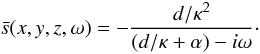
Why is the stratification altered in the boundary region? Consider for example, the
derivative term  . The differential Eq. (12) when applied to the steady
∂zp0 term leads
to:
. The differential Eq. (12) when applied to the steady
∂zp0 term leads
to: 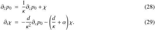 Since
we are dealing with a steady background medium, we drop the time derivative in Eq. (29) and obtain
Since
we are dealing with a steady background medium, we drop the time derivative in Eq. (29) and obtain
 (30)Note that we can
pursue a similar formalism for the gradient term
(30)Note that we can
pursue a similar formalism for the gradient term  . To maintain hydrostatic stability
in the absorption layer, we alter gravity by prefixing it by the same term,
. To maintain hydrostatic stability
in the absorption layer, we alter gravity by prefixing it by the same term,
 . And
hence the relations in Eqs. (20), (23), and (25).
. And
hence the relations in Eqs. (20), (23), and (25).
In the presence of magnetic field, three wave branches appear: magneto-sonic slow, fast, and Alfvén (the distinctions between these modes apply only if the magnetic and hydrodynamic pressures are not in equipartition). The physics of the propagation of these waves is intricate and inherently highly anisotropic (e.g., Goedbloed & Poedts 2004). Alfvén waves are transverse incompressible oscillations whereas the slow and fast modes are compressive magnetically guided/influenced oscillations. The slow mode dispersion relation exhibits certain pathologies wherein for certain wavenumbers, the phase speed vanishes while the group speed becomes very small (e.g., see pp. 195–214 of Goedbloed & Poedts 2004). This strong anisotropy destabilizes the calculation in the entry regions of the boundary layer. Thus to offset the possibility of this instability, we add the sponge term − σρ0v to the momentum equations in regions of the magnetic field.
The choice of the parameters κ,d,α is fairly central to creating an
efficient absorption boundary formulation. Following Komatitsch & Martin (2007), we set
α = πf0, where
f0 is a characteristic frequency of the waves. The
α decays linearly to zero over the absorption region, being maximum at
the start of the layer and falling to zero at the boundary. The damping function
d = f(x,y,z0) (z / L)N,
is zero at the boundary layer entry point and attains its maximum value at the boundary.
We find that for the Euler equations, the following choice for f results
in efficient absorption (e.g., Collino & Tsogka
2001):  (31)where
L is the length of the layer,
Rc is the amount of reflection tolerated,
and
(31)where
L is the length of the layer,
Rc is the amount of reflection tolerated,
and  is the characteristic sound speed in the C-PML
layer. Note that is not a function of z.
For the ideal MHD equations, we use:
is the characteristic sound speed in the C-PML
layer. Note that is not a function of z.
For the ideal MHD equations, we use:
 (32)where,
 is the characteristic propagation speed of the fastest waves in the absorption layer (set
for a specific vertical location z = z0) and
Rc,N,L retain the same
meaning as for the Euler equations. Wave propagation speeds can vary substantially from
strongly magnetized regions to non-magnetic regions; for this reason, we allow
cw to vary horizontally, i.e.,
cw = cw(x,y,z0).
The sound speed is denoted by c and the Alfvén speed by
is the characteristic propagation speed of the fastest waves in the absorption layer (set
for a specific vertical location z = z0) and
Rc,N,L retain the same
meaning as for the Euler equations. Wave propagation speeds can vary substantially from
strongly magnetized regions to non-magnetic regions; for this reason, we allow
cw to vary horizontally, i.e.,
cw = cw(x,y,z0).
The sound speed is denoted by c and the Alfvén speed by
 .
The κ term acts to damp evanescent waves (Roden & Gedney 2000; Bérenger
2002); although there are evanescent waves in our simulations, we find that
instabilities are set into motion when κ is allowed to vary from 1 at the
absorption layer entry to 8 at the boundary. For values of κ less than
this, the improvement in absorption efficiency is not very noticeable. We therefore set
κ = 1. The damping sponge is
σ = − [ (N + 1)cA / L ] (z / L)Nlog 10Rc.
The perfectly matched status of the MHD formulation comes into question with the
introduction of the sponge term. Note that because
σ ∝ cA the technique is
perfectly matched for the stratified Euler equations, i.e. for the
cA = 0 case.
.
The κ term acts to damp evanescent waves (Roden & Gedney 2000; Bérenger
2002); although there are evanescent waves in our simulations, we find that
instabilities are set into motion when κ is allowed to vary from 1 at the
absorption layer entry to 8 at the boundary. For values of κ less than
this, the improvement in absorption efficiency is not very noticeable. We therefore set
κ = 1. The damping sponge is
σ = − [ (N + 1)cA / L ] (z / L)Nlog 10Rc.
The perfectly matched status of the MHD formulation comes into question with the
introduction of the sponge term. Note that because
σ ∝ cA the technique is
perfectly matched for the stratified Euler equations, i.e. for the
cA = 0 case.
3. Numerical results
3.1. Methods
The simulation code employed in these calculations has been discussed in various previous publications (Hanasoge 2007; Hanasoge et al. 2008; Hanasoge 2008). The validation and verification of the numerical aspects of the code may also be found in these articles. In summary, to capture variations in the vertical direction, we apply sixth order, low dissipation and dispersion compact finite differences (Lele 1992). A non-uniformly spaced grid is used because the eigenfunctions change much more gradually deeper within the interior; the vertical grid spacing varies from several hundred kilometers deeper within to tens of kilometers in the near-surface layers. Because the dissipation of the scheme is low, spectral blocking occurs along the vertical directions (energy buildup at the highest wavenumbers). This is a direct consequence of the strong vertical stratification (terms like c,ρ0,p0 vary strongly with z) and the non-uniform grid spacing; in order to avoid instabilities, we regularly de-alias the variables along the z direction according to the technique described in Hanasoge & Duvall (2007). Zero Dirichlet upper and lower boundary conditions are enforced at the outer edge of the C-PMLs for all the variables. A Fourier spectral method is applied in the horizontal directions in order to compute derivatives. Time stepping is achieved through the application of a second-order optimized Runge-Kutta scheme (Hu et al. 1996). The horizontal boundaries are chosen to be periodic while the vertical boundaries are required to be absorbent. We study this case in detail below; there is no loss of generality however, since the method can be extended in order to render the horizontal boundaries absorbent as well.
An inspection of Eqs. (18) to (27) reveals that 6 memory variables are needed: for vz, the three (vector) Lorentz force components, and two in the induction equation. The memory and computational overheads are relatively small: (1) the boundary layer works well with 8–10 grid points; thus the six memory variables need only be stored over a small number of points; and (2) the additional computations are limited to a small number of multiplications and additions, as required for the evolution of the convolution Eqs. (19), (22), and (27).
3.2. Waves in a non-magnetic stratified fluid
We first demonstrate the ability of the C-PMLs at absorbing outgoing waves. The
background medium is a stratified polytrope with index m = 2.15; the
vertical extent of the computational domain is such that approximately 2.6 scale heights
in density and 3.72 scale heights in pressure fill the domain (i.e. the pressure at the
bottom is e3.72 = 41.5 times the value at the top). The
stratification properties of the polytrope are described in Appendix A.1. Waves are locally excited in a small region located at a distance
of 18 Mm above the bottom boundary (the full vertical length is 68 Mm). For the C-PML
parameters, we choose
N = 2,Rc = 0.1%,f0 = 0.005 Hz
in Eqs. (29) and (31) for these calculations. Both the upper and
lower C-PMLs are 10 grid points thick. In Fig. 1, we
show snapshots of the wavefronts at four instants of time. The scaling in all the plots is
identical. It is seen that the waves are almost completely absorbed by the upper boundary.
In order to study the absorption more quantitatively, we plot the following energy
invariant (summed over the entire grid) as a function of time in Fig. 2, (e.g., Bogdan et al. 1996):
 (33)
(33)
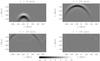 |
Fig. 1 Snapshots of the normalized wave velocity |

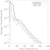 |
Fig. 2 Time evolution of the normalized modal energies as computed with Eq. (33). The initial drop in energy is due to the arrival of waves at the lower C-PML from the source.The energy of these downward propagating waves is plotted as the dot-dash line. The second drop in the energy corresponds to the first arrivals at the upper C-PML (displayed with dashed lines). Modes with large horizontal wave numbers and weakly reflected waves arrive gradually at the boundaries at later times, resulting in an extended energy decay.Both upward and downward propagating wave packets are efficiently absorbed by the CPMLs. |
We solve these equations in a computational domain of size 200 × 200 × 35 Mm3, (horizontal sides followed by vertical length) (1 Mm = 106m), discretized using 256 × 256 × 300 grid points. Vertically, the box extends from approximately 34 Mm below the solar photosphere to 1 Mm above. Standing waves or normal modes are naturally created by the stratification of the medium; the modes are trapped between the surface and a specific depth below that depends on the frequency and wavenumber of the mode. A consequence of this trapping is that the mode has an evanescent tail that extends from the surface into the overlying atmosphere. We therefore place the upper computational boundary high enough above the surface so that the normal mode evanescent tails are largely unaffected by it.
An additional aspect is that of the wave excitation mechanism: in the Sun, waves are created by the action of the strong near-photospheric turbulence (e.g., Stein & Nordlund 2000). To mimic this process, we add a horizontally homogeneous vertically localized deterministic forcing function (S of the momentum equations).This source term is only vertically directed, i.e., S = S(x,y,t)δ(z − ze)ez, where ze = − 50 km. In order to generate S, we use a Gaussian random number generator to populate its Fourier domain and the resultant function is multiplied by the average frequency power spectrum of the Sun, modeled as a Gaussian with peak frequency at 3 mHz and a full width of 1 mHz. The inverse transform of this function is S(x,y,t) (e.g., Hanasoge et al. 2006; Hanasoge 2008).
The calculation is stable over the entire time integration. The wavenumber-frequency power spectrum of the vertical velocity component vz at a height of z = 200 km above the photosphere is plotted in Fig. 3. The horizontal axis represents the non-dimensional horizontal wavenumber kh R⊙, where R⊙ is the solar radius and kh is the horizontal wavenumber, while the vertical axis is frequency in mHz.
In order to study the impact of these absorbing layers, we perform simulations with C-PMLs placed adjacent to the upper and lower boundaries (Fig. 3) and damping sponges (Fig. 4). A demonstration of the efficacy of the C-PML is the absence of artifacts related to the lower boundary in the modal power spectrum in Fig. 3. Weak reflections from the lower boundary cause the dispersion relation to change, manifested in the power spectrum as a flattening of the curvature of the ridges, as seen in Fig. 4.
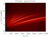 |
Fig. 3 Modal power spectrum of the vertical velocity component extracted at a height of z = 200 km above the photosphere, from a 12 h long simulation with C-PMLs placed at the upper and lower boundaries(plotted on a linear scale). The horizontal axis is the normalized wavenumber, the vertical is frequency, and regions of high power are the normal modes that appear in the calculation. The symbols overplotted on the power contours are the theoretically expected values of the resonant frequencies, computed using the MATLAB boundary value problem solver bvp4c. |
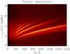 |
Fig. 4 Modal power spectrum extracted of the vertical velocity component extracted at a height of z = 200 km above the photosphere, from a 12 h long simulation with the boundaries lined by sponges(plotted on a linear scale). The weak reflections from the lower boundary cause the dispersion relation to change in curvature at all points for which ν / (kh R⊙) exceeds a certain threshold. The symbols are the same as those in Fig. 3; note that there are differences between the C-PML and sponge layered simulations at high frequencies. This is because these high-frequency waves are sensitive to the upper boundary. |
3.3. Stratified MHD fluid
We first perform a test akin to that of Fig. 2. A
constant inclined magnetic field is embedded in the polytrope of Appendix A.1; the strength of the field is such that the Alfvén
speed is approximately four times the sound speed at the upper boundary. Waves are excited
in the vicinity of the upper boundary by horizontally shaking the field lines. The fast
and Alfvén waves reach the upper boundary first but the slow modes follow behind, which
makes the demonstration of the absorptive properties of the boundary formulation less
evident than in Fig. 2. Furthermore, constructing
energy invariants for MHD waves in stratified media is not a trivial affair due to the
fairly complicated Lorentz force terms. A number of authors have studied this problem
(e.g., Bray & Loughhead 1974; Parker 1979; Leroy
1985) and have arrived at differing versions of an invariant (personal
communication, P. S. Cally 2009); we use the following approximate form (kinetic + thermal
+ magnetic energies; e.g., Bray & Loughhead
1974): 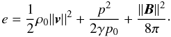 (34)We plot the time
history of the energy summed over the entire computational domain in Fig. 5.
(34)We plot the time
history of the energy summed over the entire computational domain in Fig. 5.
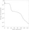 |
Fig. 5 Time evolution of the normalized MHD wave energy as computed using Eqs. (34), summed over the entire grid. Because of the strong dispersive nature of the waves and large variations in the propagation speeds between the fast, slow, and Alfvén waves, some modes take a long time to reach the boundaries, resulting in a relatively extended energy decay process compared to Fig. 2. The initial drop at t ~ 20 − 40 min corresponds to the first arrivals of waves at the upper and lower absorption layers. The secondary decline may be associated with the arrivals of the downward propagating dispersing slow and Alfvén modes at the absorption layer adjacent to the lower boundary. |
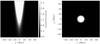 |
Fig. 6 The “sunspot” like magnetic field configuration used in the long-term integration
numerical test. On the left panel we plot the ratio of the local
Alfvén to the sound speed as a function of x and
z. The magnetic field becomes dynamically unimportant in the deeper
layers because the background hydrostatic pressure increases with relative rapidity.
The right panel displays a horizontal cut (at the solar
photosphere) through the fast mode speed ( |

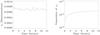 |
Fig. 7 Plotted on the left panel is the error in maintaining
| | ∇·B | | = 0 as
measured by ne, defined in Eq. (35). On the right panel
is plotted the L2 norm of
|

Our final test consists of studying the long-term stability of the method numerically. A
magnetic flux tube (e.g., Moradi et al. 2009) is
embedded in the stratified polytrope (Appendix A.2); waves are excited in the non-magnetic regions and allowed to propagate
through the flux tube, whose geometry is shown in Fig. 6. The system is stable up to 12 h of time integration. The modal power spectrum
from this data looks almost identical to that in Fig. 3 (with the exception of small frequency shifts) and is hence not shown. The
maintenance of ∇·B = 0 numerically
is an essential task of the scheme (e.g., Tóth
2000). Discretization errors are one of the primary causes for non-zero
∇·B = 0; additionally, in this
case, the boundary formulation in non
∇·B = 0 conserving. Consequently,
it is important to test if the error grows with time and to quantify its level. In order
to measure the normalized errors in maintaining
∇·B = 0, we compute the
following quantity: ![Mathematical equation: \begin{eqnarray} n_e &=& \frac{L_2\left[\int_{z_1}^{z_2}dz ||\bnabla\cdot\bB||\right]}{L_2\left[ ||\bB||\right]} \label{eq.ne}, \end{eqnarray}](/articles/aa/full_html/2010/14/aa14345-10/aa14345-10-eq117.png) (35)where
z1,z2 are the limits of the
physically-relevant domain (i.e., the non-absorbing regions) and the following definition
for the L2 norm is applied:
(35)where
z1,z2 are the limits of the
physically-relevant domain (i.e., the non-absorbing regions) and the following definition
for the L2 norm is applied:
![Mathematical equation: \begin{equation} L_2[f(x)] = \sqrt{\sum_i f(x_i)^2}, \end{equation}](/articles/aa/full_html/2010/14/aa14345-10/aa14345-10-eq119.png) (36)where the sum is over all
the grid points xi in the computational
domain. We display the time evolution of ne on the left panel
of Fig. 7. One can see that
ne is nearly constant, perhaps showing a slight decrease
with time. On the right panel we show the time history of the numerator of
ne (Eq. (35)). The gradual increase in the magnetic energy is due to constant input wave
excitation via the S term in the vertical momentum equation.
The growth rates of the magnetic energy demonstrate the numerical stability of the system
over the period of time integration.
(36)where the sum is over all
the grid points xi in the computational
domain. We display the time evolution of ne on the left panel
of Fig. 7. One can see that
ne is nearly constant, perhaps showing a slight decrease
with time. On the right panel we show the time history of the numerator of
ne (Eq. (35)). The gradual increase in the magnetic energy is due to constant input wave
excitation via the S term in the vertical momentum equation.
The growth rates of the magnetic energy demonstrate the numerical stability of the system
over the period of time integration.
4. Conclusions and future work
We have developed a Convolutional Perfectly Matched Layer (C-PML) for the stratified linearized Euler equations and a highly efficient absorption layer for the ideal MHD equations. This boundary formulation is quite useful for the calculation of wave propagation in astrophysical plasmas, where stratification and magnetic fields abound. The absorption layer for MHD waves is a slightly altered version of the convolutional formulation of (e.g., Roden & Gedney 2000), requiring an extra sponge-like term in order to stabilize the system. While the boundary methods as discussed here are perfectly matched for the stratified Euler equations, the inclusion of the sponge term casts some doubt as to whether the same could be said of the MHD equations. Simulations with the absorption layers for the stratified MHD and Euler equations were performed and found to be stable over a time length of 300 wave periods. With increasingly sophisticated boundary formulations, such as that of Hu et al. (2008), who developed the PML for turbulent flows, we may in the near future be able to extend these techniques to fully non-linear MHD turbulence/dynamo calculations.
Acknowledgments
S.M.H. is supported by the German Aerospace Center (DLR) through the grant “German Data Center for SDO”. The study on sunspot modeling is supported by the European Research Council under the European Community’s Seventh Framework Programme (FP7/2007-2013)/ERC grant agreement #210949, “Seismic Imaging of the Solar Interior”, to PI L. Gizon.
References
- Appelö, D., Hagstrom, T., & Kreiss, G. 2006, SIAM J. Appl. Math., 67, 1 [CrossRef] [Google Scholar]
- Bécache, E., Fauqueux, S., & Joly, P. 2003, J. Comput. Phys., 188, 399 [NASA ADS] [CrossRef] [Google Scholar]
- Bérenger, J.-P. 1994, J. Comput. Phys., 114, 185 [Google Scholar]
- Bérenger, J. P. 2002, IEEE Microwave and Wireless Components Letters, 12, 218 [CrossRef] [Google Scholar]
- Bogdan, T. J. 2000, Sol. Phys., 192, 373 [NASA ADS] [CrossRef] [Google Scholar]
- Bogdan, T. J., Hindman, B. W., Cally, P. S., & Charbonneau, P. 1996, ApJ, 465, 406 [NASA ADS] [CrossRef] [Google Scholar]
- Bray, R. J., & Loughhead, R. E. 1974, The solar chromosphere (Chapman and Hall) [Google Scholar]
- Cameron, R., Gizon, L., & Daiffallah, K. 2007, Astron. Nachr., 328, 313 [NASA ADS] [CrossRef] [Google Scholar]
- Cameron, R., Gizon, L., & Duvall, Jr., T. L. 2008, Sol. Phys., 251, 291 [NASA ADS] [CrossRef] [Google Scholar]
- Christensen-Dalsgaard, J. 2002, Rev. Modern Phys., 74, 1073 [Google Scholar]
- Christensen–Dalsgaard, J. 2003, Lect. Notes Stel. Oscill., 5th edn [Google Scholar]
- Collino, F., & Monk, P. 1998, Comput. Methods in Appl. Mechan. Eng., 164, 157 [Google Scholar]
- Collino, F., & Tsogka, C. 2001, Geophys., 66, 294 [CrossRef] [Google Scholar]
- Colonius, T. 2004, Ann. Rev. Fluid Mech., 36, 315 [NASA ADS] [CrossRef] [Google Scholar]
- Drossaert, F. H., & Giannopoulos, A. 2007, Wave Motion, 44, 593 [CrossRef] [Google Scholar]
- Festa, G., & Vilotte, J. P. 2005, Geophys. J. Inter., 161, 789 [NASA ADS] [CrossRef] [Google Scholar]
- Gedney, S. D., & Zhao, B. 2010, IEEE Transactions on Antennas and Propagation, 58, 838 [NASA ADS] [CrossRef] [Google Scholar]
- Gizon, L., & Birch, A. C. 2005, Living Rev. Sol. Phys., 2, 6 [Google Scholar]
- Gizon, L., Schunker, H., Baldner, C. S., et al. 2009, Space Sci. Rev., 144, 249 [NASA ADS] [CrossRef] [Google Scholar]
- Gizon, L., Birch, A. C., & Spruit, H. C. 2010, ARA&A, 48, 289 [Google Scholar]
- Goedbloed, J. P. H., & Poedts, S. 2004, Principles of Magnetohydrodynamics (Cambridge University Press) [Google Scholar]
- Hanasoge, S. M. 2007, Ph.D. Thesis, Stanford University, USA [Google Scholar]
- Hanasoge, S. M. 2008, ApJ, 680, 1457 [NASA ADS] [CrossRef] [Google Scholar]
- Hanasoge, S. M., & Duvall, Jr., T. L. 2007, Astron. Nachr., 328, 319 [NASA ADS] [CrossRef] [Google Scholar]
- Hanasoge, S. M., Larsen, R. M., Duvall, Jr., T. L., et al. 2006, ApJ, 648, 1268 [NASA ADS] [CrossRef] [Google Scholar]
- Hanasoge, S. M., Couvidat, S., Rajaguru, S. P., & Birch, A. C. 2008, MNRAS, 391, 1931 [NASA ADS] [CrossRef] [Google Scholar]
- Hu, F. Q. 2001, J. Comput. Phys., 173, 455 [NASA ADS] [CrossRef] [Google Scholar]
- Hu, F. Q., Hussaini, M. Y., & Manthey, J. L. 1996, J. Comput. Phys., 124, 177 [NASA ADS] [CrossRef] [Google Scholar]
- Hu, F. Q., Li, X., & Lin, D. 2008, J. Comput. Phys., 227, 4398 [NASA ADS] [CrossRef] [Google Scholar]
- Khomenko, E., & Collados, M. 2006, ApJ, 653, 739 [Google Scholar]
- Komatitsch, D., & Martin, R. 2007, Geophys., 72, 155 [CrossRef] [Google Scholar]
- Lele, S. K. 1992, J. Comput. Phys., 103, 16 [NASA ADS] [CrossRef] [Google Scholar]
- Leroy, B. 1985, Geophys. Astrophys. Fluid Dyn., 32, 123 [NASA ADS] [CrossRef] [Google Scholar]
- Lui, C. 2003, Ph.D. Thesis, Stanford University, USA [Google Scholar]
- Martin, R., & Komatitsch, D. 2009,Geophys. J. Int., 179, 333 [Google Scholar]
- Martin, R., Komatitsch, D., & Ezziani, A. 2008, Geophys., 73, T51 [CrossRef] [Google Scholar]
- Martin, R., Komatitsch, D., Gedney, S. D., & Bruthiaux, E. 2010, Comp. Modeling Engin. Sci., 56, 17 [Google Scholar]
- Meza-Fajardo, K. C., & Papageorgiou, A. S. 2008, Bull. Seism. Soc. Amer., 98, 1811 [CrossRef] [Google Scholar]
- Moradi, H., Hanasoge, S. M., & Cally, P. S. 2009, ApJ, 690, L72 [NASA ADS] [CrossRef] [Google Scholar]
- Parchevsky, K. V., & Kosovichev, A. G. 2007, ApJ, 666, 547 [NASA ADS] [CrossRef] [Google Scholar]
- Parker, E. N. 1979, Cosmical magnetic fields: Their origin and their activity (Oxford, Clarendon Press, New York: Oxford University Press), 858 [Google Scholar]
- Roden, J. A., & Gedney, S. D. 2000, Microwave and Optical Technology Letters, 27, 334 [Google Scholar]
- Shelyag, S., Erdélyi, R., & Thompson, M. J. 2006, ApJ, 651, 576 [NASA ADS] [CrossRef] [Google Scholar]
- Stein, R. F., & Nordlund, Å. 2000, Sol. Phys., 192, 91 [NASA ADS] [CrossRef] [Google Scholar]
- Thompson, K. W. 1990, J. Comp. Phys., 89, 439 [NASA ADS] [CrossRef] [Google Scholar]
- Tóth, G. 2000, J. Comp. Phys., 161, 605 [CrossRef] [Google Scholar]
- Werne, J., Birch, A., & Julien, K. 2004, in SOHO 14 Helio- and Asteroseismology: Towards a Golden Future, ed. D. Danesy, ESA SP, 559, 172 [Google Scholar]
- Winton, S. C., & Rappaport, C. M. 2000, IEEE Transactions on Antennas and Propagation, 48, 1055 [NASA ADS] [CrossRef] [Google Scholar]
Appendix A: Stratification
A.1. Only polytrope
For the absorption tests in Sects. 3.2 and 3.3, we use the following polytropic stratification
prescription: 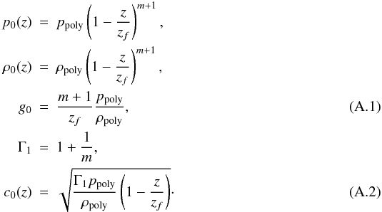 We
set
ppoly = 1.178 × 10⁵ dynes cm-2,ρpoly = 3.093 × 10⁻⁷ g cm-3,zf = − 0.450 Mm,
and m = 2.150. Note also that z is the height, i.e. the
atmospheric layers are described by z > 0 and vice versa;
z = 0 is the fiducial surface. The polytrope is truncated at
z = − 31.77 Mm (upper boundary) and z = − 104.40 Mm
(lower boundary) respectively.
We
set
ppoly = 1.178 × 10⁵ dynes cm-2,ρpoly = 3.093 × 10⁻⁷ g cm-3,zf = − 0.450 Mm,
and m = 2.150. Note also that z is the height, i.e. the
atmospheric layers are described by z > 0 and vice versa;
z = 0 is the fiducial surface. The polytrope is truncated at
z = − 31.77 Mm (upper boundary) and z = − 104.40 Mm
(lower boundary) respectively.
A.2. Polytrope + isothermal layer
Waves propagating toward the surface in the Sun are reflected by a sharp fluctuation in
the background density gradient (e.g., Christensen–Dalsgaard 2003). This reflection zone is located at a height of
zr ~ −0.050 Mm below the surface. We mimic this
by patching the polytropic stratification of Sect. A.1 with an overlying isothermal layer. This patching results in a fluctuation
in the density gradient, leading to an acoustic cut-off frequency of approximately
5.4 mHz, similar to the solar value. For
z < zM, we use
the prescription of Sect. A.1. For
z ≥ zr, we use the following equations:
![Mathematical equation: \appendix \setcounter{section}{1} \begin{eqnarray} p_0(z) &=& p_{\rm iso} \exp\left[\frac{z_{\rm r} - z}{H}\right],\nonumber\\ \rho_0(z) &=& \rho_{\rm iso} \exp\left[\frac{z_{\rm r} - z}{H}\right],\nonumber\\ \rho_{\rm iso} &=& \rho_{\rm poly} \left(1 - \frac{z_{\rm r}}{z_f}\right)^{m},\\ p_{\rm iso} &=& p_{\rm poly} \left(1 - \frac{z_{\rm r}}{z_f}\right)^{m+1},\nonumber\\ H &=& \frac{p_{\rm iso}}{g_0 \rho_{\rm iso}} \cdot \nonumber \end{eqnarray}](/articles/aa/full_html/2010/14/aa14345-10/aa14345-10-eq132.png) (A.3)The
relations for ρiso and piso arise
from the requirement of continuity of the pressure and density at the matching point
between the polytropic and isothermal layers. The relation for H is a
consequence of enforcing hydrostatic balance. This model is truncated at
z = −34 Mm (lower boundary) and z = + 1 Mm (upper
boundary).
(A.3)The
relations for ρiso and piso arise
from the requirement of continuity of the pressure and density at the matching point
between the polytropic and isothermal layers. The relation for H is a
consequence of enforcing hydrostatic balance. This model is truncated at
z = −34 Mm (lower boundary) and z = + 1 Mm (upper
boundary).
All Figures
|
Fig. 1 Snapshots of the normalized wave velocity |
| In the text | |
|
Fig. 2 Time evolution of the normalized modal energies as computed with Eq. (33). The initial drop in energy is due to the arrival of waves at the lower C-PML from the source.The energy of these downward propagating waves is plotted as the dot-dash line. The second drop in the energy corresponds to the first arrivals at the upper C-PML (displayed with dashed lines). Modes with large horizontal wave numbers and weakly reflected waves arrive gradually at the boundaries at later times, resulting in an extended energy decay.Both upward and downward propagating wave packets are efficiently absorbed by the CPMLs. |
| In the text | |
|
Fig. 3 Modal power spectrum of the vertical velocity component extracted at a height of z = 200 km above the photosphere, from a 12 h long simulation with C-PMLs placed at the upper and lower boundaries(plotted on a linear scale). The horizontal axis is the normalized wavenumber, the vertical is frequency, and regions of high power are the normal modes that appear in the calculation. The symbols overplotted on the power contours are the theoretically expected values of the resonant frequencies, computed using the MATLAB boundary value problem solver bvp4c. |
| In the text | |
|
Fig. 4 Modal power spectrum extracted of the vertical velocity component extracted at a height of z = 200 km above the photosphere, from a 12 h long simulation with the boundaries lined by sponges(plotted on a linear scale). The weak reflections from the lower boundary cause the dispersion relation to change in curvature at all points for which ν / (kh R⊙) exceeds a certain threshold. The symbols are the same as those in Fig. 3; note that there are differences between the C-PML and sponge layered simulations at high frequencies. This is because these high-frequency waves are sensitive to the upper boundary. |
| In the text | |
|
Fig. 5 Time evolution of the normalized MHD wave energy as computed using Eqs. (34), summed over the entire grid. Because of the strong dispersive nature of the waves and large variations in the propagation speeds between the fast, slow, and Alfvén waves, some modes take a long time to reach the boundaries, resulting in a relatively extended energy decay process compared to Fig. 2. The initial drop at t ~ 20 − 40 min corresponds to the first arrivals of waves at the upper and lower absorption layers. The secondary decline may be associated with the arrivals of the downward propagating dispersing slow and Alfvén modes at the absorption layer adjacent to the lower boundary. |
| In the text | |
|
Fig. 6 The “sunspot” like magnetic field configuration used in the long-term integration
numerical test. On the left panel we plot the ratio of the local
Alfvén to the sound speed as a function of x and
z. The magnetic field becomes dynamically unimportant in the deeper
layers because the background hydrostatic pressure increases with relative rapidity.
The right panel displays a horizontal cut (at the solar
photosphere) through the fast mode speed ( |
| In the text | |
|
Fig. 7 Plotted on the left panel is the error in maintaining
| | ∇·B | | = 0 as
measured by ne, defined in Eq. (35). On the right panel
is plotted the L2 norm of
|
| In the text | |
Current usage metrics show cumulative count of Article Views (full-text article views including HTML views, PDF and ePub downloads, according to the available data) and Abstracts Views on Vision4Press platform.
Data correspond to usage on the plateform after 2015. The current usage metrics is available 48-96 hours after online publication and is updated daily on week days.
Initial download of the metrics may take a while.